


As finance returns to its fundamental purpose of serving the real economy, its connections with various industries are strengthening. Accurately depicting the interdependence among these industries and mitigating financial risks has become increasingly critical. The dependence among China's real industries is dynamic rather than static, which is particularly pronounced during the COVID-19 pandemic. In this paper, we propose a dynamic factor model to optimize the risk of high-dimensional portfolios. To describe the dependence structure, we employ the factor copula model, driven by a GAS (Generalized Autoregressive Score) model. By combining the dynamic factor model with a mean-ES (Expected Shortfall) model, we construct a dynamic factor copula-mean-ES model. Our empirical findings, based on an analysis of 24 industries in China, suggest that the dynamic heterogeneous factor copula model is the most suitable for describing portfolio risk. Furthermore, the mean-ES model ensures the lowest portfolio risk for a given expected return. Accurate return predictions enable leveraging market information to develop a "good knowledge" of dynamic copula and risk optimization. This "good knowledge" of dynamic copulas facilitates precise return prediction and effective risk optimization of portfolios, thereby addressing the relationship between risk prevention and sustainability. Moreover, it reveals the internal connection between China's real industry and the risk landscape of the financial market.
The COVID-19 pandemic has profound impact on the economy, leading to a prolonged market downturn and presenting significant challenges for the Chinese economy. The real economy, a crucial pillar of national development, currently faces financing difficulties due to its extended production cycle. Thses challenges has been further exacerbated by the pandemic's restrictions on production time and space. In a bid to support the development of the real economy and promote a stable decline in total financing costs, the central bank announced a reduction of 0.25 percentage points in the required reserve ratio of financial institutions, effective from April 25, 2022. This measure aims to release approximately 530 billion yuan in long-term funds by implementing a broad-based reduction in the required reserve ratio. The central bank has emphasized its commitment to maintaining a prudent monetary policy while considering the overall situation.
With the sustained and stable development of the market economy in China, the interdependence among different industries is increasingly prominent. Each industry has a significant impact on others and collectively contributes to an integrated economic community. Furthermore, the dynamic growth of financial markets and proactive policy implementation have established a foundation for enhancing service to the real economy. This has facilitated the organic integration of financial services with the real economy, reinforcing the interconnection between finance and the real economy. However, the proliferation of financial risk events has expanded in a more extensive and profound manner, making risk measurement and prevention increasingly complex.
Given the robust policy support and the growing integration of financial services with the real economy, it is crucial to promote the stable growth of the real economy in an increasingly interconnected market economy and seize the opportunities presented by favorable policies. Since each industry plays a vital role in the real economy, it is worthwhile to examine their respective development paths. Therefore, this paper aims to investigate the correlation among the 24 industries classified under first-level industry classification of Shenwan in China and their impact on the real economy. This study evaluates the changes in risks faced by China's actual industries and provides recommendations to bolster the real economy.
This paper proposes a novel model that combines the dynamic factor copula model with the mean-ES model for studying high-dimensional portfolio optimization. The paper makes two main contributions. First, it improves upon existing high-dimensional dependency measurement methods. Previous research mainly focused on dependency relationships among low-dimensional asset portfolios and faced challenges when dealing with high-dimensional investment portfolios, resulting in difficult parameter estimation due to the “curse of dimensionality”. This paper introduces the GAS model into the dynamic factor copula model, addressing the parameter estimation problem of high-dimensional investment portfolio assets with complex dependencies. Second, it enhances portfolio risk optimization methods. Recognizing the significant impact of asset dependency relationships on portfolio risk optimization, this paper combines the dynamic factor copula model with traditional risk optimization models, constructing a mean-ES model based on the dynamic factor copula. This model obtains asset weight vectors with minimum portfolio risk for three types of dependency relationships, providing a "good knowledge" of the role of dynamic dependence relationships in portfolio risk optimization.
The remainder of this paper is structured as follows. In the subsequent section, we will provide an overview of the relevant literature. Following this, we will introduce our theoretical framework and present our novel model. Moreover, we will present the empirical results and provide interpretations of our findings. Finally, we will summarize our conclusions and suggest potential avenues for future research.
Literature reviewDynamic factor copulaSklar (1959) pioneered the use of copula functions to model complex dependencies and address the challenge of characterizing dependence relationships among multiple assets. Embrechts et al. (2002) were the first to introduce copulas in financial risk management, and since then, copulas have become a widely employed analytical tool in the financial and insurance domains. In a recent study, Chen et al. (2022) examined the dynamic connection between the international crude oil market and China's nonferrous metal market using a change-point detection copula method.
Dimensionality reduction is crucial for constructing a dependent structure model with high-dimensional variables. Vine copula (Bedford & Cook, 2001) and factor copula (Krupskii & Joe, 2013) are two specific approaches to achieve this goal. Vine copula models, which combine the graphical tools of the "vine" with pair copulas, are often used to characterize the interdependent structure of stock markets (Du, 2009; Wu et al., 2013; Fan et al., 2013; Zhang et al., 2014; Gong & Deng, 2015; Guo, 2017; Wei & Wei, 2018; Xu et al., 2019). On the other hand, some scholars have utilized factor copula models to represent the interdependent structure in credit portfolio risk through common factors (Su & Furman, 2017; Chen et al., 2020).
However, the two methods mentioned above are applicable to different dimensions. The vine copula model is primarily used to address dependence among data with dimensions lower than 12 (Song et al., 2019). Conversely, the factor copula model reduces the parameter complexity of the model through the factor structure, transforming high dimensions into low dimensions (Wang & Yuan, 2017). Additionally, there are significant correlations among industries in the Chinese stock market, and the factor copula model can be extended to the real industries in China, playing a crucial role in studying the structure of dependence.
The financial market is subject to rapid changes due to various influences, particularly in response to major political or economic events. It is inadequate to rely solely on a single structure or parameter copula model to depict the dynamic correlation of the financial market (Gong & Shi, 2011; Zhang et al., 2022). The generalized autoregressive scoring (GAS) model is a data-driven approach for modeling time-varying parameters proposed by Creal et al. (2013). It encompasses a range of time-varying parameter modeling issues within the same framework, providing a novel approach to modeling copula functions. Numerous studies have utilized copula models within the GAS framework to capture the dynamic dependence structure (Zou & Fan, 2018; Li & Kang, 2016; Song et al., 2020; Zhao et al., 2021; Oh & Patton, 2017).
Studies on the dynamic factor copula model have primarily focused on credit default swaps and systemic risk in banks, with no previous application to the analysis of real industries. In this paper, our aim is to contribute to the literature by utilizing the dynamic factor copula model to depict the dynamic interdependence among multiple real industries in optimizing market risk. By doing so, we aim to develop a "good knowledge" of the role of dynamic dependence relationships in this context.
The role of the dynamic factor copula in forecasting returnsBaumol (1963) originally proposed value at risk (VaR) as a risk measure, which represents the potential loss of a specific financial asset or portfolio at a certain confidence level over a specific period. However, VaR does not satisfy the properties of a consistent risk measure as proposed by Artzner et al. (1999) when returns do not follow a normal distribution. To address this limitation, Rockafellar and Uryasev (2002) introduced expected shortfall (ES), a risk metric that captures tail information beyond VaR and covers the exposure of risk in extreme market situations. They transformed the optimization problem into minimizing continuously differentiable functions that connect VaR and ES. Forecasting the return of each asset is an essential component of risk optimization based on the mean-ES model. Therefore, it is necessary to capture the dependence structure among the returns of different assets.
Zhang (2004) used the copula function to calculate VaRs for optimizing portfolio risk. To enhance the effectiveness of risk measurement, several scholars have combined copulas with other risk measurements in portfolio optimization. For instance, Boubaker and Sghaier (2013) employed the copula method to examine the impact of long memory on portfolio optimization. Deng and He (2017) integrated pair copulas with the mean-ES model to explore optimal strategies for market portfolios. Feng and Ou (2012) illustrated the asymmetrical tail correlation among financial markets using the SJC copula and utilized the CVaR to determine the efficient frontier and optimal strategy of asset portfolios. Bekiros et al. (2015) employed the vine copula to model the interdependence structure of portfolios during the financial crisis in three periods and optimize portfolio risk.
Based on the literature mentioned above, research on portfolio risk optimization has yielded advanced findings and has been widely implemented in various fields. However, accurate dependence relationships are crucial for portfolio risk optimization. Currently, the mean-ES model is primarily combined with traditional copula functions or vine copula models. Further research is needed to investigate the combination of the mean-ES model and the dynamic factor copula model. In this paper, our aim is to examine the impact of the mean-ES model on portfolio risk optimization based on dynamic factor copula models of various dependence types, in order to explore the effect of different dynamic factor copula models on asset portfolio optimization. It is important to consider the combination of the dynamic factor copula model and the mean-ES model in the study of portfolio optimization.
MethodologyThis section will present the theoretical basis of the analysis presented in this paper. We will introduce the dynamic factor copula model and use it as the basis for constructing the mean-ES model.
Dynamic factor copula modelWe consider an n-dimensional vector Y=[Y1,Y2,⋯,YN]′ with joint distributions F, marginal distribution Fi, and a copula function C:

Following the construction principle of the factor model, the data generation process of potential variables Xi is given by the following simple factor structure:
where Z represents the common factor, εi denotes the idiosyncratic variable, and C is the factor copula. This type of factor model is considered to be more flexible and practical compared to the factor model proposed by Li (2000).


Oh and Patton (2017) describe the dynamics of parameters in the factor copula using the GAS model. The GAS model is specifically designed to adapt to the joint distribution of multiple variables, offering significant advantages in modeling dynamic dependencies in high-dimensional scenarios. The dynamic factor copula model can be illustrated as follows:
where Xt=[X1t,X2t,⋯,XNt]′, Zt represents the common factor, εit,i=1,2,3,⋯N denotes the idiosyncratic variable, C is the factor copula, and λit(γλ) is the ith factor loading at time t. The GAS model for logarithmic factor loadings is given by:


The model would have N + 2 parameters requiring estimation without considering the parameters of Fεt and FZt. This can result in significant computational complexity, particularly when N is sizeable. To address this issue, Oh and Patton (2018) introduced the variance targeting (VT) method under the assumption of a strictly stationary sequence {λt}. Eq. (8) can be rewritten as
where E[logλit]=ωi1−β. Eq. (11) effectively reduces the number of parameters to be estimated and resolves the issue of "dimension disaster".Mean-ES model based on the dynamic factor copula

With the evolution of financial practices, the use of variance as a method of measuring risk has consistently revealed inadequacies. Consequently, alternative and superior risk measures have progressively replaced variance. In this paper, we use ES as a replacement for variance and implement the mean-ES model to examine the portfolio optimization problem. ES represents the conditional expected value when the loss is below a given level of significance (Artzner et al., 1999). To be precise, ES can be defined as follows:
where ft(rt) is the density function of the return rt. We assume u=Ft(rt), where 0

Rockafellar and Uryasev (2002) introduced a consistent risk measure called ES, which demonstrates both subadditivity and convexity. They also established a connection between VaR and ES using a unique function. The definition of this function is as follows:
where w represents the weight vector, r represents the vector of asset returns with probability density function is p(r), f(w,r) represents the loss function, and α is the portfolio VaR value at the confidence level 1−β. By minimizing the function Fβ(w,α), the value of (w*,α*) can be determined. According to Rockafellar and Uryasev's (2002) findings, the weight w* is associated with the minimum ES, while α* represents the corresponding VaR value. In practice, since the distribution of returns r is often unknown, the returns rk,k=1,2,⋯M for M cases can be obtained using Monte Carlo simulation. Eq. (14) can be approximately transformed into the following form:

In the field of portfolio risk optimization, Markowitz (1952) pioneered the concept of an optimal portfolio that balances risk and return. His fundamental idea is that if investors expect a portfolio return that is not inferior, then optimization should focus on minimizing risk. Conversely, if investors aim to control the risk of exceeding the expected value, then optimization should prioritize maximizing returns. Building upon this principle, we propose the mean-ES model based on the dynamic factor copula. In this model, we aim to minimize risk while the achievement of the expected return. The model takes the following specific form:


It is important to note that the returns rk,k=1,2,⋯M are generated based on the dynamic factor copula model, wi represents the corresponding optimal weight, n is the number of study variables, and μp is the expected return. This model forms the foundation for the development of "good knowledge".
Empirical resultsDataThis paper focuses on 24 industries classified according to Shenwan's first-level industry classification in China. These industries covers a wide spectrum: agriculture, forestry and fishing (abbreviated as AFF), mining, chemical, steel, nonferrous metal, electronics, household appliance, food and beverage, textile and clothing, light manufacturing, pharmaceutical biology, public utilities, transportation, leisure services, synthesis, building material, building decoration, electrical equipment, defense industry, computer, media, communication, car, and machinery. These industries represent leading enterprises in their respective sectors. The sample period for index returns spans from December 1, 2011, to December 1, 2021. The data were obtained from the iFinD database and analyzed using R language and MATLAB.
The daily logarithmic return of each industry index is calculated according to rit=logpit−logpi,t−1. The value of pit is the closing price of the industry index i on a specific day t, generating a total of 2438 sample groups of daily logarithmic returns.
Subsequently, a time series graph depicting the daily logarithmic returns for the 24 industry indices is plotted. This graphical representation facilitates an analysis of the fluctuation characteristics exhibited by each index, providing insights into their respective returns. Fig. 1 illustrates the time series diagram illustrating the logarithmic returns for the 24 industry indices.

Based on the observations from Fig. 1, it is evident that the 24 industry indices display a consistent asymmetric return trend, indicating a strong correlation among the industries. Notably, significant fluctuations occurred in 2015 and 2020, primarily attributed to the global stock market crash in 2015 and the substantial impact of COVID-19 pandemic on the stock market in 2020.
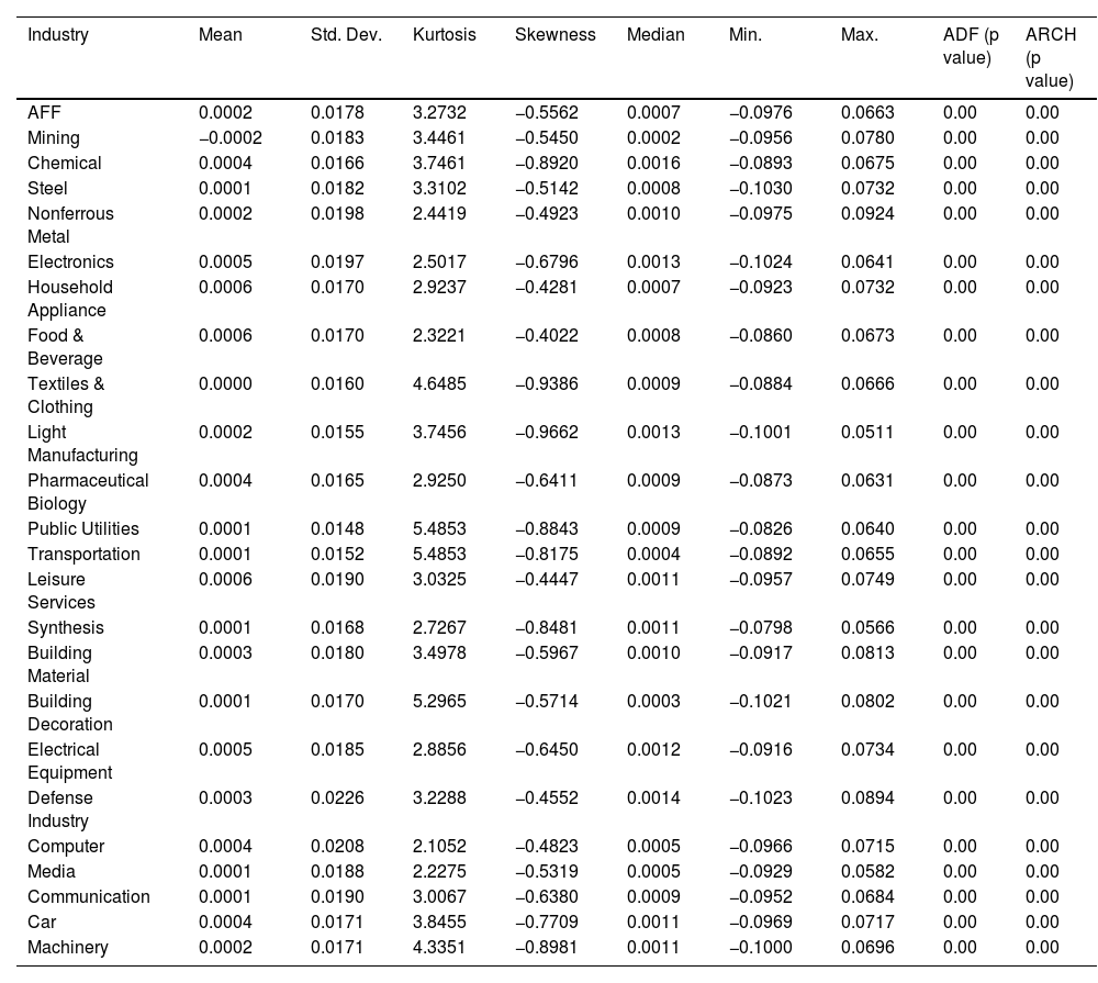
Table 1 presents the mean, standard deviation, kurtosis, skewness, median, minimum, and maximum values of the daily logarithmic return for the 24 industry indices. Additionally, tests are conducted to assess the stationarity and volatility clustering within these returns.
Summary statistics of the index returns.
According to the results in Table 1, the ADF test rejects the null hypothesis for the stability of returns in the 24 industry indices, indicating stability at a 1% significance level. Furthermore, the ARCH effect test showed that the returns of the 24 industry indices did not reject the presence of an ARCH effect.
Marginal distributionsConsidering the presence of leptokurtosis, asymmetry, and volatility clustering in financial time series, this paper utilizes the AR-GARCH model to capture the characteristics of the returns’ marginal distribution. Moreover, the residuals are assumed to follow a t distribution. The model's explicit expression is presented as follows:
where rt and rt−1 are the returns at times t and t−1, respectively. σt2 is the conditional variance of at.


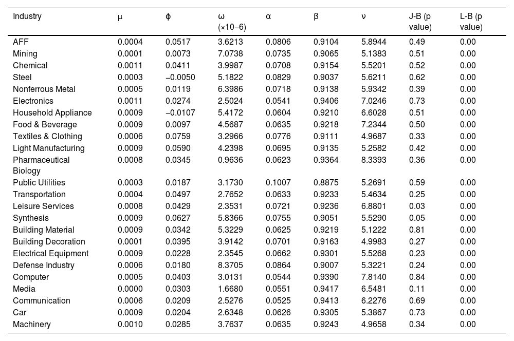
The estimated parameters of the marginal distributions are used to analyze the returns. The results of the Jarque-Bera test suggest non-normal distributions in returns. Additionally, to validate the suitability of the AR-GARCH model, the Ljung-Box test is employed to verify that the residuals conform to a white noise sequence. The results of the Jarque-Bera and Ljung-Box tests are presented in Table 2.
The parameter estimation results for the AR-GARCH model.
Based on the findings presented in Table 2, the results of the Jarque-Bera test indicate that none of the residuals associated with the 24 industry indices followed a normal distribution, as evidenced by the rejection of the null hypothesis for all of them. Furthermore, the Ljung-Box test revealed no significant autocorrelation in any of the 24 residuals at the 1% significance level. Additionally, the residuals exhibited characteristics of white noise sequences, indicating that the AR-GARCH model provided a reasonably good fit.
Dependency analysisIn this section, we employ the dynamic factor copula model to estimate the dynamic dependence structure among real industries. We consider three different structure: equidependence, block dependence, and heterogeneous dependence structures, aiming to compare the differences in the dependent structure across these models. We assume that the common factor Z follows a skewed distribution, while the idiosyncratic variables ε follow a t distribution. This generates three unknown parameters. To estimate these parameters through maximum likelihood estimation, we refer to the work of Oh and Patton (2018).
In the dynamic factor copula model of equidependence, ωi(i=1,2,⋯,N) remains constant in Eq. (11). This model involves only six parameters. The specific form of the model is as follows:


The parameter estimation for the dynamic homogeneous factor copula model using maximum likelihood estimation is presented in Table 3.
Table 3 displays the results of maximum likelihood estimation for parameter estimation of the dynamic equidependence factor copula model.
In the dynamic block dependence factor copula model, the time-varying parameter in Eq. (11) is determined based on the grouping situation, where identical values are assigned to the same group of ωi(i=1,2,⋯,N). This model yields 5 + M parameters, with M representing the number of groups. The specific form of the model is as follows:
where λgt denotes the factor load under different groups, and Eq. (23) is the time-varying equation of the factor load for each group.

Considering the significance of the real industry in the country's economy, this paper has categorized the 24 indices into six well-balanced groups. The results of the cluster analysis are presented in Table 4.
Classification of various industries of the real industry.
In this case, M = 5, and a total of 10 parameters are generated for the dynamic block dependence factor copula using maximum likelihood estimation, as shown in Table 5.
In the dynamic heterogeneous dependence factor copula model, the time-varying parameters ωi(i=1,2,⋯,N) in Eq. (11) are not equal. This model generates N + 5 parameters, and the specific model form is as follows:
where λit represents the factor loads of different potential variables, and Eq. (25) represents the time-varying equation for each factor load.

In the case of the heterogeneous dependence model, a large number of parameters are involved in the dynamic factor copula model when dealing with high-dimensional data. To reduce the computational complexity, Oh and Patton (2018) employed the variance targeting (VT) method to calculate ωi. The calculation is as follows:

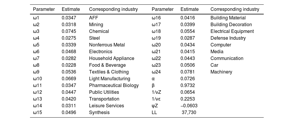
The estimated results are shown in Table 6.
Parameters estimates of the heterogeneous dependent factor copulas.
Tables 3-6 illustrates that the dynamic factor copula model, encompassing equidependence, block dependence, and heterogeneous dependence structure, provides an enhanced representation of the dynamic interdependence among the 24 industry indices. Specifically, it was discovered that the log-likelihood of the dynamic heterogeneous dependent factor copula model attained the highest value, indicating a superior fit. Building upon the copula model of real industry dependence, this paper further investigates the portfolio optimization within China's real industry.
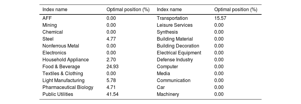
Portfolio optimizationBuilding upon the previously mentioned interdependence among the real industries, the Monte Carlo method generates 20,000 sets of random weight vectors. These weights are then used to calculate the corresponding expected returns and risks. By utilizing the effective frontier theory, the portfolio with minimum risk is identified. Therefore, Table 7 displays the optimal position ratios for the minimum-risk portfolio.
Optimal position ratios.
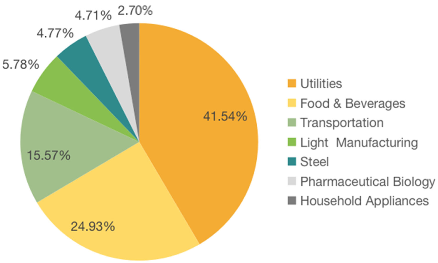
Based on the information presented in Table 7, it can be observed that public utilities industry holds the largest proportion in the minimum-risk portfolio, accounting for 41.54%. Following this, the food and beverage industry and transportation industry follow, representing the second and third largest shares at 24.93% and 15.57%, respectively. Further clustering analysis distributes the seven industries into six distinct groups. This suggests a relatively low correlation among the industries, as detailed in Table 4.
Specifically, public utilities are categorized into Group 5, while food and beverage as well as transportation are grouped into Group 6, recognized as typical defensive industries. Light manufacturing belongs to Group 3, which is associated with industrial production. Steel is part of Group 1, representing the industrial branch. Pharmaceutical biology is included in Group 4, representing emerging industries. Lastly, household appliance is placed in Group 2, encompassing electronics and appliances. These classifications align with the mean-ES model, which asserts that hedging risk and enhancing returns require weak dependence among the assets in the portfolio. Therefore, it highlights the feasibility of portfolio optimization using the mean-ES model, and its theory is consistent with the observed scenario.
The aforementioned conclusion can be more intuitively visualized through Fig. 2.

Fig. 2 illustrates that the portfolio with the minimum risk in China encompasses the country's pillar industries, which cater to our essential daily needs. Public utilities include industries such as water, power, and heat supply, and their stable operation and sustainable growth contribute to the promotion of the economic system and meeting the housing demand.
Food and beverage is closely tied to people's lives and hold significant economic value. Transportation provides essential support for economic development and growth. Light manufacturing represents a traditional and advantageous industry in China's economy, catering to the clothing needs of the population.
Pharmaceutical biology serves as a pillar of China's economy and an emerging industry meeting the increasing health demands of an aging population. Supported by the government, pharmaceutical biology has evolved into a high-tech sector that fulfills the requirement of medical field.
Intelligent home appliances have become indispensable tools for creating a comfortable living environment, with chips playing a pivotal role in their functions and addressing specific customer needs. Household appliance has been significantly impacted by global economic dynamics and policies, including technological sanctions and the global shortage observed in developed countries.
Steel products are fundamental materials extensively used in various industries related to food, clothing, housing, and medicine. During the pandemic, China's steel industry played a crucial role in facilitating the rapid recovery of the national economy due to its robust and abundant production capacity. However, it also exemplifies a high-energy consumption and high-emission sector within the industrial landscape. With the carbon peaking and carbon neutrality goals in mind, there is increased pressure and a substantial challenge to reduce carbon emissions. This necessitates the adoption of targeted reform measures for steering China's steel industry toward low-carbon development.
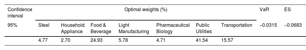
By using the optimal weights from Table 7, the VaR and ES for the optimal portfolio were calculated at a 5% significance level, and the results are presented in Table 8.
Table 8 illustrates that at a 5% significance level, the ES of the optimal portfolio is significantly smaller than the VaR, indicating that ES effectively capture extreme losses. When evaluating risk, it is essential to concentrated on the lower tail of extreme risk using ES as a measure.
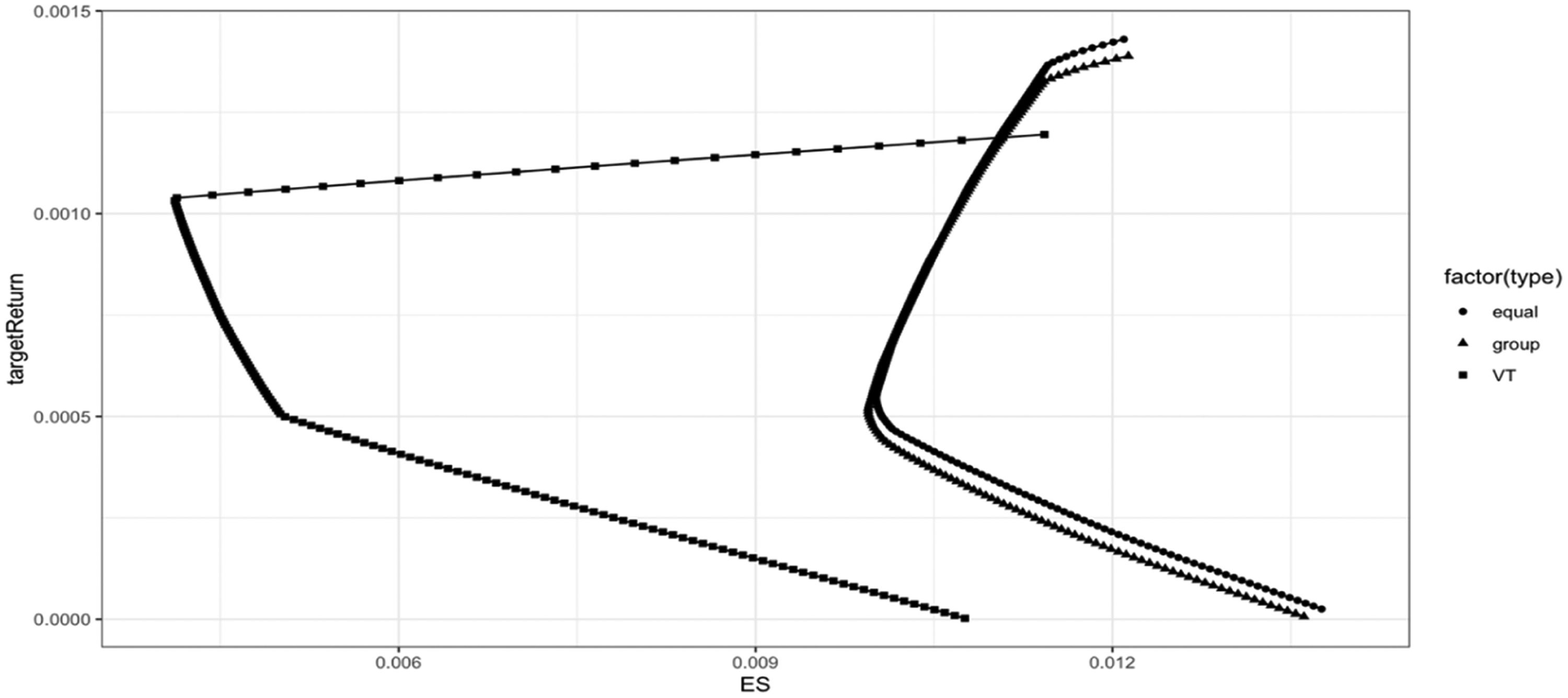
This paper undertakes a comparative analysis of the efficient frontier generated by the mean-ES model across three dynamic factor copula models. The comparison results are shown in Fig. 3.

Fig. 3 illustrates the variations in the efficient frontier calculated using three dynamic factor copula models. The dynamic heterogeneous dependence factor copula model exhibits a more pronounced discrepancy in the effective frontier compared to the other two dynamic factor copula models.
If the expected return falls below 0.0012, the efficient frontier of the dynamic heterogeneous dependence factor copula model is positioned to the left of the other two models, exhibiting its lower risk while maintaining a consistent expected return. Conversely, when the expected return exceeds 0.0012, the efficient frontier of the dynamic heterogeneous dependence factor copula model shifts to the right of the other two models. This shift correlates with an increase in the ES of the dynamic heterogeneous dependence factor copula model as the expected return rises. Consequently, as the expected return grows, this model effectively mitigates risk by accurately. These findings highlights the crucial impact of characterizing the dependent structure among real industries on portfolio optimization.
The expected return is derived based on the optimal weight provided in Table 8. A basic statistical analysis is then conducted, and the results are presented in Table 9.
Under the mean-ES model, the three dependent structures produce distinct expected returns. In particular, the dynamic heterogeneous dependence factor copula model exhibits the highest mean expected return and the smallest variance. This signifies the capacity of the dynamic heterogeneous dependence factor copula model to generate a superior and more consistent return. As a result, this model maximizes returns while minimizing portfolio risk by an accurate characterization of the dependencies among real industries.
We proceed to evaluate the accuracy of the minimum VaR and minimum ES that were acquired for the three corresponding dependent structures. The results of the test at a significance level of 5% are presented in Table 10.
The findings in Table 10 demonstrate that the minimum VaR and minimum ES based on the three dependent structures successfully pass the test at a 5% significance level. This suggests that the dynamic copula models, specifically the equidependence, block dependence, and heterogeneous dependence factor copula models, are better suited to capture the dynamic dependence among the 24 real industries. Notably, the p value associated with the dynamic heterogeneous factor copula model is the highest, indicating that the VaR and ES based on this model are the most accurate.
In the ES test, the p value of the dynamic heterogeneous factor copula model exceeds 0.05, indicating acceptance of the null hypothesis. These test results suggest the superior performance of the dynamic heterogeneous factor copula model over the other two models in risk optimization studies using ES as a risk metric. In conclusion, a “good knowledge” of the mean-ES model can greatly enhance the accuracy of risk measurement. Furthermore, the risk metric ES proves to be more precise than VaR.
ConclusionWe construct a dynamic factor copula-mean-ES model to explore the relationship among real industries in China and examine the impact of dynamic connections on optimizing portfolio risk. The empirical results are as follows.
First, the three dynamic factor copula models constructed in this study accurately measure risk in portfolio optimization. Particularly, the dynamic heterogeneous factor copula model demonstrates the highest accuracy in estimating the minimum ES by effectively characterizing the dependence relationship among China's real industries. This highlights the "good knowledge" gained regarding the role of dynamic dependency relationships in portfolio risk optimization.
Second, in the analysis of portfolio risk optimization, the public utilities industry holds the largest weight. This is due to its inclusion of industries such as water, power, and heat supply, which exert a significant influence on national economic development. Conversely, the mining sector holds the smallest weight as it is highly influenced by downstream nonferrous metals and steel, facing increased risks due to the rapid development of new energy sources. Although this study focuses solely on China without incorporating data from other countries, the model shows promising applicability for future economic research due to the shared nature of financial data.
DiscussionResearch on financial risk is a significant and timely topic in the current academic field. China places a high importance on its real economy and consistently implements policies to support its growth. In this context, it is crucial to promote the steady development of the real economy in an increasingly interconnected market. This paper utilizes the dynamic factor copula model to measure the financial risk within the real industry and examines its portfolio optimization problem. The empirical analysis has yielded insightful conclusions. However, it is important to note that a country's financial market operates within a broader global context and is subject to various external factors. Future research could incorporate factors from other countries, taking into account the risk contagion effect. This would provide investors and relevant government departments with more comprehensive and effective information.
FundingThis work was supported by Zhejiang Province Philosophy and Social Science Planning Routine Subject (24NDJC131YB), Zhejiang Provincial Natural Science Foundation of China (LY21G010003), the National Natural Science Foundation of China (12371150, 11971432), Zhejiang Provincial Natural Science Foundation of China (LQ22G010001), the Zhejiang Provincial Philosophy and Social Sciences Planning Project (22YJRC07ZD-2YB), Zhejiang Provincial Research Project of Statistics (22TJQN07). The management project of "Digital+" discipline construction of Zhejiang Gongshang University (SZJ2022A012, SZJ2022B017). This work was also supported by the Characteristic & Preponderant Discipline of Key Construction Universities in Zhejiang Province (Zhejiang Gongshang University-Statistics) and Collaborative Innovation Center of Statistical Data Engineering Technology & Application.