An application of extreme value theory in estimating liquidity risk

Abstract

The last global financial crisis (2007–2008) has highlighted the weaknesses of value at risk (VaR) as a measure of market risk, as this metric by itself does not take liquidity risk into account. To address this problem, the academic literature has proposed incorporating liquidity risk into estimations of market risk by adding the VaR of the spread to the risk price. The parametric model is the standard approach used to estimate liquidity risk. As this approach does not generate reliable VaR estimates, we propose estimating liquidity risk using more sophisticated models based on extreme value theory (EVT). We find that the approach based on conditional extreme value theory outperforms the standard approach in terms of accurate VaR estimates and the market risk capital requirements of the Basel Capital Accord.

1

Introduction

As a response to the financial crisis of 2008–2009, the Basel Committee on Bank Supervision (BCBS) proposed a review of the supervisory framework for market risks and introduced new requirements for the trading book (BCBS, 2011a, 2012, 2013, 2016). The new capital requirements assume: (a) a considerable tightening of existing capital requirements; (b) a reduction in arbitrage between bank banking and trading books; and (c) limiting the procyclical effects of such bank capital requirements. The use of internal models was allowed, but the BCBS announced the reconsideration of the VaR concept as the basis of capital requirement for market risk calculations.

The change in the supervisory framework constitutes a response to the fact that during the last crisis, it was found that many financial institutions had insufficient resources to cover the market risk losses they faced during this period. As many such institutions use VaR to quantify their market risk exposure, such results may suggest that this measure may not be appropriate for estimating risk.

Among others factors, the failure of the VaR measure in quantifying risk may be attributable to the fact that many risk management systems estimate VaR from the distribution of portfolio returns computed at the bid-ask average price. This method underestimates risk by neglecting the fact that liquidation occurs not at bid-ask average prices but rather at bid prices. The asset bid price is calculated by adding liquidity costs of an asset to the ask-bid average price. Thus, when liquidity costs are high, which is observed in the financial crisis period, differences between bid and bid-ask average prices become very pronounced. In such cases, estimating VaR using average prices may cause one to underestimate risk.

In taking this into account, the academic literature has proposed incorporating liquidity risk in estimations of market risk (Bangia, Diebold, Schuermann & Stroughair,1999; Ernst, Stange, & Kaserer, 2008, 2009; Stange & Kaserer, 2008). Market liquidity risk emerges as a consequence of changes in liquidity costs. As stated above, these costs can increase dramatically during a financial crisis.

The financial industry and even the BCBS have echoed such proposals (BCBS, 2011b). In this document it is discussed the possibility of requiring financial institutions calculate market risk capital requirement on the bases of VaR adjusted by liquidity risk. In this context, properly measuring liquidity risk is a fundamental task.

In the aforementioned papers, liquidity risk is quantified using the Value at Risk measure. Bangia et al. (1999) defined the liquidity cost as the mid-point of the spread, and they used the VaR of the relative spread as a measure of liquidity risk. Thus, the value at risk adjusted by liquidity costs is calculated by adding the relative spread relative to the price risk.

In this paper, we follow Bangia et al. (1999) by approaching liquidity costs based on the average of the spread, and we estimate liquidity risk as the worst liquidity cost. In their study, Bangia et al. (1999) use a parametric method below a normal distribution to estimate spread VaR. The empirical literature has shown that the spread distribution is far from normal, presenting high levels of skewness and kurtosis. Therefore, the parametric method based on a normal distribution may underestimate liquidity risk. As a way to overcome the drawbacks of this approach, Ernst et al. (2008) propose using a non-normal distribution for relative spread that is estimated from a Cornish–Fisher expansion approximation.

As we show below, the tail of the empirical spread distribution can be adequately characterized by a method based on extreme value theory. Therefore, as a way to estimate properly liquidity risk, we propose using conditional extreme value theory to estimate spread VaR and compare the corresponding results with those obtained by the Ernst et al. (2008) propose. The results indicate that conditional extreme value theory outperforms the parametric method both in terms the accuracy of VaR estimations and of daily capital requirements.

The remainder of the paper is organized as follows. In Section 2, the methodology used to estimate liquidity cost and risk is described. Section 3 presents the empirical analysis conducted. Section 4 present the capital requirements are analyzed. The last section presents our main conclusions.

2

Methodology

2.1

Liquidity cost

Liquidity in financial markets implies the ability of a particular asset to be traded in the market over a considerably short period of time with a minimal loss of value (Kyle, 1985). Many risk management systems assume that a position can be bought or sold without cost when the liquidation horizon is long enough. However, in real financial markets, liquidity costs can be substantial.

Market risk is basically concerned with describing price/return uncertainty resulting from market movements. Bangia et al. (1999) split risk in the market value of an asset into two components: uncertainty arising from asset returns (pure market risk component) and risk due to liquidity risk.¹

Liquidity cost is defined as the cost of trading an asset relative to its fair value where the fair value is defined as the bid-ask average price Pmid,t². According to this definition, liquidity cost (COL_t) at time t is calculated as follows:

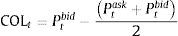
While taking into account that the bid price is given by (Ptbid=Pmid,t−(1/2)Ptask−Ptbid), the liquidity cost (COL) is calculated as follows:

where Ptask−PtbidPmid,t is the relative spread. In the following sections, we denote this expression as S_t.

The expression (2) for liquidity cost is correct for small positions but not for larger positions, as market markers are only required to trade positions of up to a certain size at the quoted spread. As a consequence, in the case of larger positions, liquidity cost measured by the average of the spread can be underestimated. In solving this problem, some proposals have been made; see, for instance, Berkowitz (2000), Cosandey (2012) and Giot and Grammig (2006). For a review of these approaches, see Stange and Kaserer (2009). All these proposals consider the fact that liquidity costs increase with the size of the position beyond the quoted spread. The problem with these approaches concerns the data necessary for their implementation, which are not readily available. Spite, the quoted bid-ask spread is not a precise measure of liquidity cost for larger positions, in this paper, we use this approach, as it is overwhelmingly used by companies due to the ease of access to data, thus resulting in cost savings when incorporating liquidity risk while quantifying market risk.

2.2

Measuring market risk

Prices and returns are described through the following typical framework:

where P_mid,t is defined as the mid-price at time t and where r_t is the continuous daily mid-price return at time t, i.e., r_t = ln(P_mid,t/P_mid,t−1). In this paper, we use the Value at Risk (VaR) measure to quantify market risk so that we can define the risk price as the relative VaR at the (1 − α) percent confidence level over a 1-day horizon:

where rtα is the α-percentile of daily distribution returns. Thus, VaRreturnsα measures the maximum percentage loss over a 1-day horizon with a confidence (1 − α) percent.

In this paper, we use two alternative models to estimate risk price: RiskMetrics (Morgan, 1996), which is a very simple model, and a more sophisticated approach based on conditional extreme value theory (EVT).³

Empirical literature show that EVT performs very well in estimating VaR, while RiskMetrics performs very poorly at this task (see Abad, Benito, & López, 2014). In this paper, we use these two models because we wish to evaluate whether the impact of incorporating liquidity risk is dependent on how well we estimate risk prices.

Under RiskMetrics, the Value at Risk of an asset at α % probability can be calculated as:

where μ and σ_t are the unconditional mean and conditional standard deviation of the returns; k_α is the percentile α of the standard normal distribution. For the estimation of conditional volatility (σ_t), we use the exponentially weighted moving average model (EWMA) proposed by Morgan (1996). Assuming that financial returns {r_t} follow a stochastic process r_t = μ + σ_tε_t, εt∼iii0,1 where σt=Eεt2Ωt−1 and that ε_t has a conditional distribution function Gε where Gε=Prεt<εΩt−1, the Value at Risk of an asset below the conditional extreme value theory can be calculated as follows:

where μ and σ_t are the unconditional mean and conditional standard deviation of the returns, respectively, and where Gα−1 is the α-percentile of the generalize Pareto distribution (for a more detailed description of this method, see Abad et al., 2014). For the estimation of conditional volatility (σ_t), we use an EGARCH model below a student-t distribution.⁴ In contrast with the EWMA model, this model captures most characteristics of financial returns (the fat tail, cluster in volatility and leverage effects).

2.3

Incorporating liquidity risk to market risk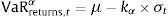

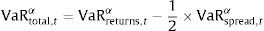
To incorporate liquidity risk when measuring market risk, we follow Bangia et al. (1999) by adding the worst liquidity cost to the price risk. Thus, we assume that in adverse market environments, there is a perfect correlation between extreme events in returns and event extremes in the spread.⁵ Thus, the liquidity-adjusted total risk is defined as:

Bangia et al. (1999) assume that the relative spread follows a normal distribution and estimate the VaR of the relative spread as:

where s˜ and σ˜t are the unconditional mean and conditional standard deviation of the relative spread, respectively, and where z_α is the α-percentile of the normal standard distribution. As we show below, the relative spread distribution is far from normal, presenting a high degree of skewness and kurtosis. Thus, using a parametric method under a normal distribution may cause one to underestimate liquidity risk. To overcome this drawback, Ernst et al. (2008) propose using a non-normal distribution for relative spread that is estimated using a Cornish–Fisher expansion approximation. Under this approach, the VaR of the relative spread is calculated as:

where z˜α is the non-normal-distribution percentile adjusted for skewness and kurtorsis according to the Cornish–Fisher Expansion (CFE):

where γ is the skewness and k is the excess of kurtosis of the respective distribution. Ernst et al. (2008) show that this approach yields more precise risk forecasts than the original specifications of Bangia et al. (1999). In this paper, we use conditional extreme value theory to estimate relative spread VaR, and we compare these estimations with those obtained from the method proposed in Ernst et al. (2008).

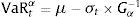
Assuming that relative spread data {s_t} follow the stochastic process s_t = μ_s + σ_s,tε_tεt∼iii0,1 where σt=Eεt2Ωt−1 and ε_t have a conditional distribution function G(ε) where Gε=Prεt<εΩt−1, the value at risk of the relative spread under conditional extreme value theory can be calculated as follows:

where μ_s and σ_s,t are the unconditional mean and conditional standard deviation of the relative spread and where Gα−1 is the α-percentile of the generalize Pareto distribution. For the estimation of the conditional volatility of the relative spread, we use a GARCH⁶ model (Bollerslev, 1986). To test the accuracy of the VaR estimate, we use several standard tests: unconditional (LRuc), independence (LRind), conditional coverage (LRcc) and the Dynamic Quantile (DQ) test (see Abad et al., 2014). In addition, we evaluate the VaR estimate based on daily capital requirements (see McAleer, Jiménez, & Pérez, 2013). These authors adapt to daily terms of the function used by financial institutions to calculate market risk capital requirements over a 10-day horizon (Basel II). The daily capital requirement at time t can be calculated as follows (BCBS, 1996, 2006):

where DCR_t denotes the daily market capital requirement at time t, which is the higher value between −k×VaR¯60 and −VaR_t−1; VaR¯60 is the mean VaR over the previous 60 working days; and (3 ≤ k ≤ 4) is the Basel II violation penalty⁷

3

Empirical application

3.1

Data analysis

For our empirical analysis, we use data from six telecommunications companies: Singapore Telecom, Samart Telcoms (Thailand), Telekom (Malaysia), Orange (France), Telefónica (Spain) and Vodafone (United Kingdom). The data include closing daily bid and ask prices extracted from the DataStream database. Mid prices are calculated as the average of bid and ask prices. These prices are transformed into returns by taking logarithmic differences. The relative spread is calculated as the difference between bid and ask prices divided by the mid-price.⁸

The analysis period run from January 2000 to the end of September 2015. The full data period is divided into a learning sample (from the start of the series to December 31, 2007) and forecast sample (January 1, 2008 to December 31, 2009). This forecast period was chosen because it is characterized by a period of significant global volatility known as the Financial Global Crisis period.

The analysis if the descriptive statistics of the daily return of the bid price and the spread indicate that both the distribution of the returns and the spread distribution is asymmetric and exhibit an important excess of kurtosis (fat tail and peaknesss).⁹

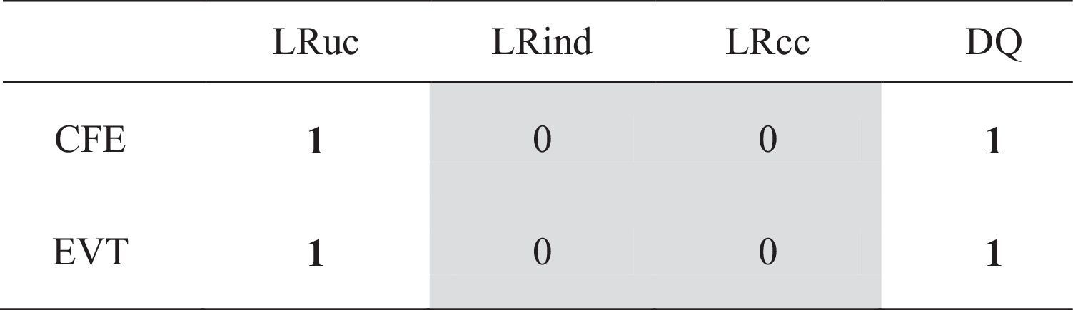
3.2

Analysing relative spread VaR

In this paper, liquidity risk is measured though the VaR of relative spread. Thus, in this section, we focus on evaluating the performance of models used for his estimation, which include the Cornish-Fisher expansion (CFE) approximation and the approach based on conditional extreme value theory (EVT). VaR was calculated 1 day ahead at the 99% confidence level according to the BCBS market risk framework. The analysis period runs from 1 January 2008 to the end of December 2009.

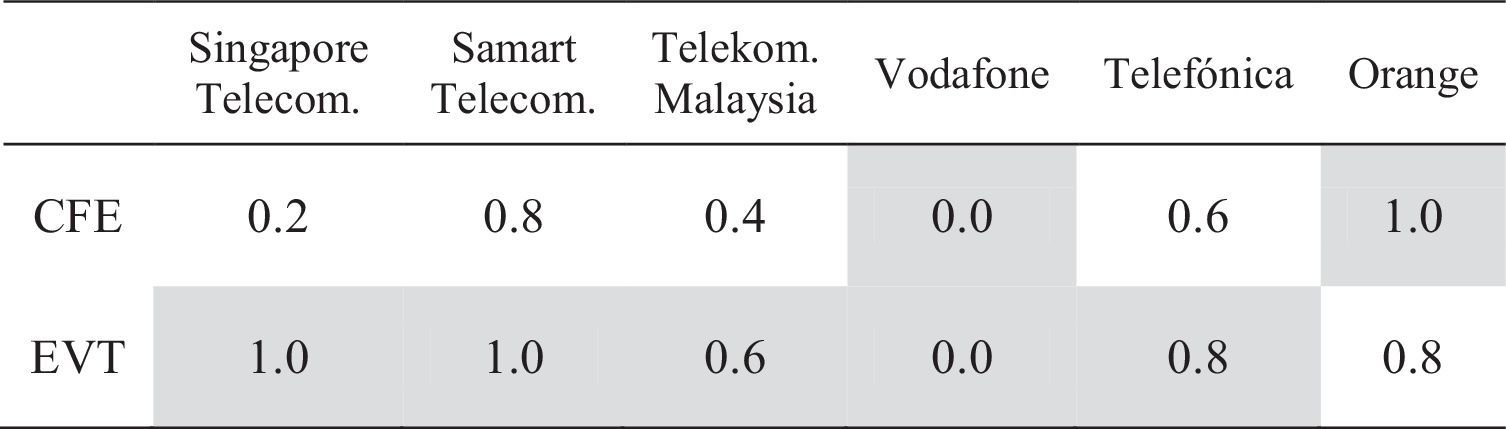
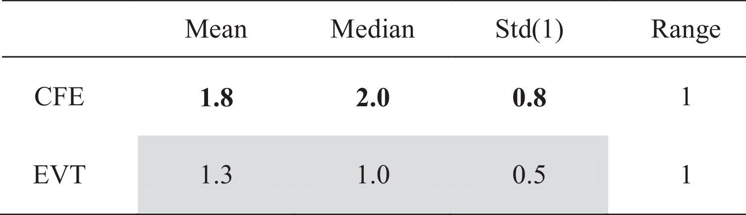
To test the accuracy of the VaR estimate, we use several standard test (LR_UC, LR_CC, LR_IND and DQ). Table 1 counts the number of rejections for each model over 6 assets at the 1% level for each of the four tests considered. These results indicate that both models provide accurate VaR estimates, as this hypothesis is rejected in just two cases. The accuracy test helps us determine whether a model provides accurate estimates or not, but this tool reveals nothing about how well a model performs compared to others. Thus, to identify differences between both models (CFE and EVT), we follow Gerlach, Chen, and Chan (2011) and focus on analysing the VRate/α ratio and on descriptive statistics of this ratio (Tables 2, 3 and 4). The VRate/α ratio is calculated as the quotient of percentage exception by the value of α, which is 1%. Under CFE approximation, the VRate/α ratio is different and less than 1 across the 5 assets, denoting that this approach overestimates risk in all cases (Table 2). The approach based on conditional EVT generates ratios closest to 1 and equal to 1 in some assets (Singapore Telecom and Samart Telcoms). It seems that this last approach performs much better. Table 3 shows VRate/α summary statistics for each model across the 6 assets. The Std (1) column shows the standard deviation from the expected ratio of 1 (not the mean sample) while the 1st column counts assets for which the model generated a VRate/α closest to 1. The results confirm the above conclusion. Under CFE approximation, the mean and median are more distant from 1 (0.5), and the standard deviation from 1 is 0.6. This approach ranks first in only two cases. Under the approach based on conditional EVT, the mean and median of VRate/α are close to 1 (0.7 and 0.8, respectively) with a standard deviation from 1 equal to 0.5. In addition, this approach ranks first in 5 cases. To help distinguish between the better models, Table 4 shows summary statistics on each approach in terms of how close its VRate/α is to 1 across the assets. For ratios that are equidistant from 1, conservative ratios (less 1) are preferred. Mean, median, standard deviation values measured from 1, and the ranking of each approach are presented. For both approaches and for the confidence levels considered, the CFE is the worst model because it generates by far the highest mean rank (1.8), the highest median rank (2), and a standard deviation of 0.8 away from 1. For the EVT approach, statistics come close to a value of one: mean (1.3), median (1) and a standard deviation (0.5) less than that of the CFE.

Table 1.

Counts of model rejections for four tests, across the 6 assets, for the spreads.

Note: Shaded cells indicate the favourable model and bold figures indicate the least favourable model, in each column.

Table 2.

Spreads ratio VRate/α for each VaR model across the 6 assets.

Note: Shaded cells indicate closest to 1 in that asset.

Table 3.

Spreads summary statistics for the ratio VRate/α for each VaR model.

Note: Shaded cells indicate the most favourable model for being closer to one.

Table 4.

Spreads summary statistics for model ranks, in terms of Vrate/α, across the 6 assets.

Note: Shaded cells indicate closest to 1 in that assets. Bold figures indicate the worst model, each columns. Std(1) is the standard deviation in ratios from an expected value of 1.

Overall, we conclude that although in terms of accurate tests we do not find differences between both approaches, a detailed analysis of the VRate/α ratio provides evidence in favour of the approach based on conditional extreme value theory.

3.3

Analysing VaR returns

As we show in Section 2.3, the VaR adjusted by liquidity risk was calculated by adding the worst liquidity cost to the risk price (Eq. (7)). For the estimation of price risk, we use RiskMetrics and the approach based on conditional extreme value theory (conditional EVT). For the estimation of liquidity risk, we use two alternative models: (a) Cornish-Fisher expansion (CFE) approximation and (b) conditional extreme value theory (EVT). By combining the estimations of these four models, we obtain VaR adjusted by liquidity risk in the following four cases: (i) RiskMetrics adjusted by liquidity risk calculated under CFE approximation (RiskM_adj_CFE); (ii) RiskMetrics adjusted by liquidity risk calculated under conditional EVT (RiskM_adj_EVT); (iii) conditional EVT adjusted by liquidity risk calculated under CFE approximation (CEVT_adj_CFE) and (iv) conditional EVT adjusted by liquidity risk calculated under conditional EVT (CEVT_adj_EVT).

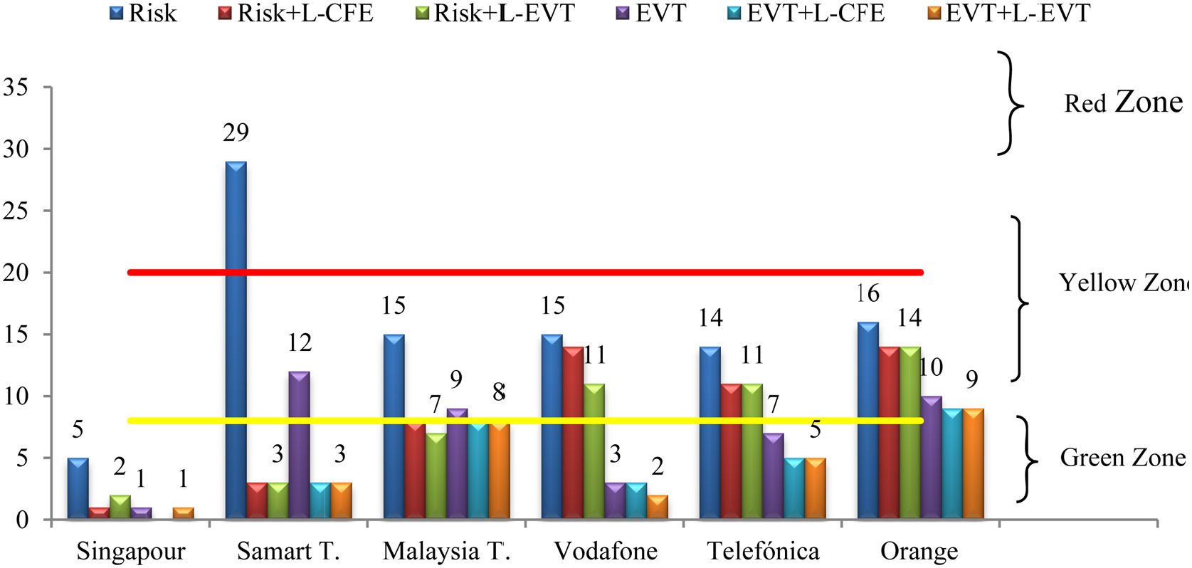
For all these models and for RiskMetrics and the conditional EVT used for estimating risk price (a total of six), we calculate the Value at Risk 1 day ahead at 1% probability, and we evaluate the accuracy of the estimations. The analysis period runs from January of 2008 to the end of December of 2009. In Fig. 1, we present the number of exceptions for all assets considered. As was expected, RiskMetrics performed very poorly in estimating VaR. According to this method, the number of exceptions occurring in 2008–2009 is far from the five expected (see Fig. 1). According to Basel II (2006),¹⁰ this model is positioned in the yellow zone for all assets. When we incorporate liquidity risk into the risk price and use a simple model for estimating risk price as RiskMetrics, the accuracy of the VaR estimate improves considerably, especially for companies operating in emerging countries. Thus, RiskMetrics adjusted by liquidity risk independent of how it estimates CFE and/or EVT moves to the green zone for Singapore, Samart Telcoms and Malaysia T. However, for Vodafone and Telefónica, RiskMetrics adjusted by liquidity risk keep on the yellow zone. This may be attributable to the fact that the liquidity component is reduced for companies in developing countries so that the incorporation of liquidity risk into price risk has no significant effects.¹¹ Regarding conditional EVT, it seems that this model performs very well in estimating VaR, reaching the green zone for all assets with the exception of Samart T. and Orange. In this case, the incorporation of liquidity risk in estimating VaR does not appear to generate significant improvements. In the following lines, we present a more rigorous analysis of these models by analysing the VRate/α ratio and accuracy test.

Fig. 1.

Number of violations in analyzed period (2008–09). Note: The figure shows backtesting results obtained with each model. BIS assigns regulatory capital according to the number of violations an institution's market risk model experiences over a year. The institutions assigned a regulatory colour (green (0–4 exceptions), yellow (5–9) and red (10 or more)). In the figure the limit of this zone have been marked but taking into account twice for these violations because we have estimated VaR in two years (2008–2009). (For interpretation of the references to colour in this figure legend, the reader is referred to the web version of the article.)

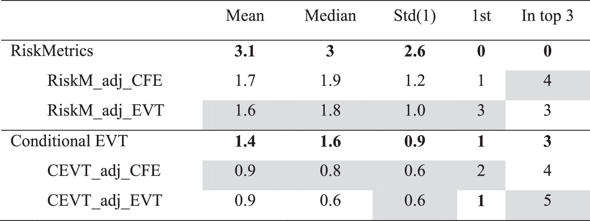
From a comparison between RiskMetrics and conditional EVT approaches, without taking liquidity risk into account, conditional EVT generates better results (Table 5). For five of the six assets, conditional EVT generates the ratio VRate/α closet to one. According to this ratio, RiskMetrics underestimates risk in five cases. What occurs when we incorporate liquidity risk into the estimation of price risk? A comparison between RiskMetrics, RiskM_adj_CFE and RiskM_adj_EVT shows that the latter two models generate more VRate/α ratios that are closer to one than RiskMetrics, indicating that in this case, the accuracy of VaR estimates improves considerably when liquidity risk is incorporated into risk price estimates. A comparison between RiskM_adj_CFE and RiskM_adj_EVT shows that the model we propose for estimating liquidity risk generates the best results. On the other hand, a comparison between conditional EVT, CEVT_adj_CFE and CEVT_adj_EVT shows that the latter two methods generate a VRate/α ratio closest to one, although the differences are not as significant. In this case, the model we propose for estimating liquidity risk does not outperform the standard approach (CFE). Our analysis of the statistics descriptive of these ratios (Table 6) reinforces the above results.

Table 5.

Ratio VRate/α at α = 1% for each VaR model across the 6 assets.

Note: Shaded cells indicate closest to 1 in that assets. Bold figures indicate the worst model.

Table 6.

Summary statistics for the ratio VRate/α for each VaR model.

Note: Shaded cells indicate closest to 1 in that assets. Bold figures indicate the worst model, each columns. Std(1) is the standard deviation in ratios from an expected value of 1 ‘1st’ indicates the number of assets where that model's VRate ratio ranked closest to 1. ‘In top 3’ counts the number of assets where the model's VRate ratio ranked in the top 3 model.

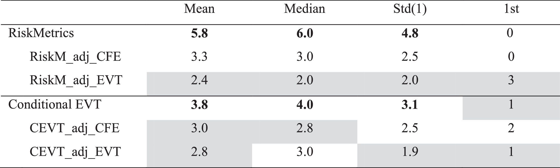
In Table 7, we present summary statistics on the ranking of each approach in terms of how close its VRate/α ratio is to 1 across the considered assets. RiskMetrics is the worst model, as it has the highest mean and median rank (5.8). Estimates improve when we use RiskMetrics adjusted by liquidity risk calculated with conditional EVT (RiskM_adj_EVT); when using this approach, the mean and median rank are 2.4 and 2, respectively. A comparison between conditional EVT, CEVT_adj_CFE and CEVT_adj_EVT shows that the results improve slightly when liquidity risk is incorporated into the risk price. A comparison between CEVT_adj_CFE and CEVT_adj_EVT shows that the model we propose for estimating liquidity risk generates the best results.

Table 7.

Summary statistics for model ranks, in terms of VRate/α across the 6 assets.

Note: Shaded cells indicate closest to 1 in that assets. Bold figures indicate the least favourable model, in each column. Std(1) is the standard deviation in ranks from the value of 1.

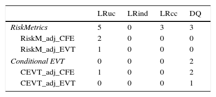
The accuracy of the VaR estimate was also analyzed through an accuracy test. In Table 8, we present the number of times that the “accurate VaR estimate hypothesis” has been rejected for each of the four tests considered. The accuracy tests corroborate the conclusions gleaned from Tables 5, 6 and 7. RiskMetrics was rejected through several of the tests. In fact, the LR_UC test rejects the “accurate VaR estimate hypothesis” for five assets. For RiskM_adj_EVT and CEVT_adj_EVT, the number of rejections is minimal at only zero and one, respectively.

Table 8.

Counts of model rejections for four tests, across the 6 series.

	LRuc	LRind	LRcc	DQ
RiskMetrics	5	0	3	3
RiskM_adj_CFE	2	0	0	0
RiskM_adj_EVT	1	0	0	0
Conditional EVT	0	0	0	2
CEVT_adj_CFE	1	0	0	2
CEVT_adj_EVT	0	0	0	1

Note: Shaded cells indicate the favourable model and bold figures indicate the least favourable model, in each column.

As a conclusion of this section we find that when risk price is estimated from a simple model, such as RiskMetrics, the incorporation of liquidity risk in estimating VaR notably improves results, especially in the case of companies operating in emerging countries. However, when risk price is estimated from advance methods, such as the conditional EVT, consideration of liquidity risk barely improves results and may cause one to overestimate risk. Furthermore, when the risk price is calculated from a simple model, VaR estimates adjusted by liquidity risk are better when liquidity risk is estimated based on conditional EVT.

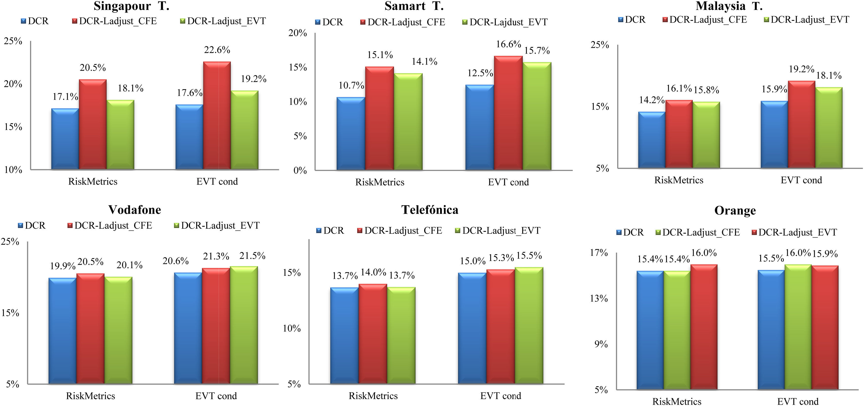
4

Daily capital requirements

In this section, we compare VaR estimates in terms of daily capital requirements (DCR) calculated according equation (14).¹² A comparison between RiskMetrics and conditional EVT shows that this last approach generates much higher DCR values than RiskMetrics. The differences between these two models range between 0.5% and 1.8% depending on the asset concerned. Thus, although conditional EVT has been shown be superior to the RiskMetrics approach in terms of accurate VaR estimates, banks may have no incentives to use this methodology, as this approach forces them to uphold more capital requirements.

Fig. 2.

Average daily capital requirements. NOTE: The figures show the average daily capital requirement obtained according to Eq. (7). DCR indicates that approaches calculated by RiskMetrics and conditional EVT have not taken into account the liquidity risk. DCR_Ladjust_CFE (DCR_Ladjust_EVT) indicates that liquidity risk has been estimated by CFE(EVT).

On the other hand, as was expected, the incorporation of liquidity risk into risk price independent of how it was measured increased DCR. This increase is especially critical in the case of companies operating in emerging countries. The incorporation of liquidity risk increases the average DCR by 3.4 percentage points (p.p.) for Singapore Telecom, by 4.4 p.p. for Samart Telecom and by 1.9 p.p. for Malaysia T. These values are obtained when we use RiskMetrics to estimate risk price and Cornish–Fisher Expansion approximation to estimate liquidity risk. However, in the case of companies operating in developed countries such as Vodafone and Telefónica, the application of liquidity risk increases DCR by no more than one percentage point. These differences between companies are attributable to the fact that the liquidity component is very high among companies operating in emerging countries but smaller in the case of companies operating in developed countries. In the case of companies operating in emerging countries, we find that independent of how risk price is measured, DCR values are higher under Cornish-Fisher expansion approximation when estimating liquidity risk than conditional EVT. We can thus conclude that DCR values are very sensitive to the model that we used to estimate risk price and liquidity risk. Regarding the risk price model, conditional EVT generates higher DCR values than RiskMetrics. On the other hand, regarding liquidity risk, CFE approximation generates higher DCR values than conditional EVT.

In our opinion, all these results should be considered by regulators. If banks wish to increase market risk capital requirements, they should carry out their policies with a stronger emphasis on the use of more precise measurements. As Rossignolo, Fethi, and Shaban (2012) show, regulators worldwide should be interested in techniques and metrics that manage large fluctuations (most notably EVT) and should discourage the use of traditional methodologies that only provide capital buffers for common market variations (essentially linear models and normal specifications).

5

Conclusion

The most recent global financial crisis (2007–2008) has stressed the weaknesses of Value at Risk (VaR) as a measure of market risk, as this measure by itself does not take liquidity risk into account. In an attempt to address this problem, the academic literature has proposed incorporating liquidity risk into the estimation of market risk by adding the VaR of the spread to the risk price. The parametric approach is the standard approach used to estimate liquidity risk. As this approach does not generate reliable VaR estimates, we propose estimating liquidity risk using more sophisticated models, such as the method based on extreme value theory. Therefore, in this paper, we evaluate the role of conditional extreme value theory in estimating risk price and liquidity risk. The results of this model are compared with those of standard approaches (RiskMetrics for risk price and Cornish–Fisher expansion for liquidity risk). Regarding risk price, we found that the approach based on conditional value theory is superior to the standard approach (RiskMetrics) in estimating VaR, as the performance of the latter method is very poor when applied for this purpose. However, the approach based on the conditional extreme value theory takes the banks to keep more capital charge by fixing daily capital requirement bigger than RiskMetrics. As a consequence, banks may have no incentive to efficiently estimate risk price. Regarding liquidity risk, we found that the approach based on conditional extreme value theory outperforms the Cornish–Fisher expansion (CFE) approximation in spread VaR estimation. In addition, this method takes to the banks to keep fewer capital charges than CFE approximation.

This study highlights another interesting issue. Liquidity component is very high in the case of companies operating in emerging countries, ranging at approximately 30% depending on the asset. This highlights the need to consider this component when measuring market risk. However, for companies operating in developed countries, using this component in estimating risk price not appear, to be as essential. In these cases, regulators may prefer to encourage banks to be more efficient at estimating risk prices that incorporating liquidity risk in calculation of market risk.