Previous research on the effects of constraints to take unbounded positions in risky financial assets shows that, under the logarithmic utility function, multiplicity of equilibrium may emerge. This paper shows that this result is robust to either constant, decreasing or increasing relative risk aversion obtained under the generalized logarithmic utility function.
The effect of portfolio constraints and capital market imperfections on financial asset pricing equilibrium is a key topic on financial economics. This type of analysis is especially relevant after the turmoil experienced by financial markets in the last three years.
There are three main strands of literature dealing with the effects of portfolio constraints on financial equilibrium. A recent particularly relevant research analyzes the impact of portfolio constraints on the international propagation of adverse shocks. Pavlova and Rogobon (2008) show how portfolio constraints amplify stock price fluctuations among international stock exchange markets. As expected, absent of portfolio constraints, all co-movements are due to the common stochastic discount factor and the term of trade channels. However, once portfolio constraints are in place, the authors characterize a dynamic equilibrium model in which an excess co-movement in stock prices relative to the unconstrained economy naturally arises. Moreover, they are able to associate their results with the contagion phenomenon previously studied in literature.
The second strand is the literature on asset pricing models with different types of frictions and market imperfections. The effects of portfolio constraints on equilibrium asset and consumption allocations typically include short-sales, borrowing, liquidity constraints, and restricted participation. Examples are Jarrow (1980), He and Pearson (1991), He and Modest (1996), Heaton and Lucas (1996), Detemple and Murphy (1997), Basak and Cuoco (1998), Basak and Croitoru (2000), Kogan and Uppal (2001), Detemple and Serrat (2003), Scheinkman and Xiong (2003), Gallmeyer and Hollifield (2008), and Bhamra and Uppal (2009). An overall conclusion of this literature seems to indicate that short-sale constraints may lead to higher equity volatilities whereas borrowing-constrained equilibria typically leads to lower equity volatilities,1 and that frictions generate a wedge between the stochastic discount factor and asset prices large enough to make some well-known empirical puzzles compatible with equilibrium in financial markets.
Finally, a third related strand, which is especially relevant for this paper, investigates the effects of portfolio constraints on the multiplicity of financial equilibrium. Basak et al. (2008) (BCLP hereafter) are the first to investigate the extent to which portfolio constraints to take unbounded positions in risky assets generate multiplicity or even indeterminacy of equilibria. They show that the introduction of this type of constraints increase the number of equilibria in the economy. In particular, they demonstrate that under potentially complete markets and portfolio constraints, there may be a finite number of additional equilibria over and above the efficient original financial equilibrium. Moreover, under incomplete markets and portfolio constraints, there is also a continuum of them, with consumption allocations varying across this continuum. Indeed, as BCLP (2008) point out, under these circumstances, there may be robust real indeterminacy of equilibrium.
The finding that portfolio constraints may expand the set of equilibria, even though by itself it does not imply equilibrium indeterminacy, is a particularly relevant result because it may help to understand, within a rational framework, the large fluctuations of asset returns which are difficult to explain simply by changes in economic fundamentals.2 If a financial market with binding portfolio constraints admits more than one but still a finite number of equilibria for the same economic fundamentals, variability of stock prices could be entirely due to investors’ expectations. Thus, excess volatility or market crashes may be explained by rational expectation-generated phenomena, with investors selecting a particular equilibrium over another.
BCLP consider a simple pure-exchange two-period model, with two goods, two households, two states of nature (in the complete markets case) and two stocks paying off in units of the goods. In the incomplete markets case an additional state is incorporated, leaving the number of financial assets and the number of goods unchanged.
Interestingly, households are characterized as heterogeneous agents in the sense of having different marginal propensity to consumption, and different initial endowments specified in terms of shares of stocks, not goods. More importantly, only one of the household faces a portfolio constraint to take unbounded positions on the holdings of one of the risky assets. Otherwise, no more restrictions are considered; in particular, short sales are permitted. Unfortunately, however, the household preferences are described by a Cobb–Douglas log-linear utility function. Indeed, as BCLP recognize, this may be a rather restrictive assumption since this utility functions presents decreasing absolute risk aversion, but constant relative risk aversion. While the issue of the realistic sign of absolute risk aversion has been settled for a long time, the direction of relative risk aversion remains an open question. This suggests that a satisfactory model should be tolerant of different attitudes of relative risk aversion.
The contribution of this paper is to investigate the robustness of equilibrium multiplicity with portfolio constraints under a more general and flexible utility function.3 Along these lines, Rubinstein (1975) convincible argues that a successful asset pricing model should require decreasing absolute risk aversion, and tolerate increasing, constant, or decreasing relative risk aversion. He shows that the generalized logarithmic utility function is a particularly attractive model since it satisfies this requirement and, at the same time, it allows a pricing expression for an uncertain intertemporal cash flow stream even when this is serially correlated over time. Furthermore, the asset pricing model under this type of preferences assumes no exogenous intertemporal stochastic process of asset prices. For a given household h, and a single consumption good, the generalized logarithmic utility function is given by,
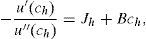
where uh(·) is the utility of household h, Ch is the consumption of the available good, and Jh is an exogenous taste parameter that may take different signs. This is the key parameter that captures heterogeneity among households since it simultaneously tolerates increasing, constant or decreasing relative risk aversion depending upon Jh is positive, zero or negative, respectively.4 Therefore, Jh will be referred to as the measure of household risk-preference; the higher Jh, the more risk preferring the household. It is also the case that, when Jh≤0, the household will never consume for Ch≤−Jh, since such low levels of consumption have infinite disutility. Hence, when Jh≤0, −Jh may be interpreted as the subsistence level of consumption. Finally, this utility function belongs to the Hyperbolic Absolute Risk Aversion (HARA) or linear risk tolerance class of tastes and it represents the solution to the differential equation,for B=1.5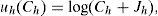
In this paper, we extend the model of BCLP (2008) when the households are characterized by the log-linear generalized logarithmic utility function with different propensities to consume. For the case of two households, and two goods, the utility function is given by,
where, as before, uh is the utility of each household h characterized by decreasing absolute risk aversion; Chg is the consumption of the good g by household h; αhg is the marginal propensity to consume the good g by household h, and Jhg is the taste parameter representing either increasing (Jhg>0), constant (Jhg=0), or decreasing (Jhg<0) relative risk aversion.
The main result of this paper is that the multiplicity of equilibria remains for all Jhg. This implies that large movements in financial markets may be related to the effects of portfolio constraints on equilibrium prices.
The rest of the paper is organized as follows. Section 2 describes the basic model and shows the results in the complete markets case. Section 3 analyzes the effects of incomplete markets. Finally, Section 4 concludes the paper.
2Generalized logarithmic utility and portfolio constraints: the complete market case2.1The basic modelIn this section we present the fundamental model and the main results of the paper. We borrow from BCLP (2008) the notation and the novel approach to obtain the equilibrium. We assume a basic pure-exchange economy with two-time periods, t=0 and 1. Uncertainty is represented by two states of the world in t=1, ω=u (up) and d (down), occurring with probabilities π(ω). When it will be useful to refer to the initial period of the economy as another state of world, these will be labeled by ϕ=0, u, d.
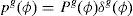
There are two non-storable goods, labeled g=1, 2, with prices Pg(ϕ)>0. The production of each good g is modeled as a Lucas (1978) tree, with the exogenously specified stream of output δg(ϕ)>0. Financial investment opportunities are given by two risky stocks, with period 0 prices qg(0), which are claims to the outputs of the two trees. Each stock is in constant supply of one unit.
There are two households in the economy, indexed by h=1, 2. Each household is endowed with an initial portfolio of the two stocks shg(0) and trades in spot markets for goods in periods t=0, 1 and the stock market in the initial period t=0. The unique restriction imposed on the households’ portfolios is the portfolio constraint on household 2. In particular, household 2 faces a portfolio constraint of the form s22(1)≥f(·). This constraint implies that household 2 cannot take unbounded positions in stock two. This type of restriction is very common in institutional investments. Both mutual and pension funds have diversification restrictions that forbids them to hold more than a given percentage of the total fund in a given stock. As in BCLP (2008), we also consider an endogenous portfolio constraint; that is, we make the right-hand side of the portfolio constraint, f(·), depend on the endogenous variables of the model. Apart from this one, no more restrictions are imposed (in particular, short sales are permitted).
Each household chooses its consumption of the goods, Chg(ϕ)>0, and terminal portfolio holdings, shg(1), using the log-linear generalized logarithmic utility function given by
where β>0 is the discount factor and we note that, from now on and for convenience, we employ the following new parameters, αh1=ah, αh2=1−ah, ah∈(0, 1). The heterogeneity of households’ utilities (a1≠a2) is required for our results. In addition, it is assumed that a1>a2 and that the discount factor is common across households for simplicity.
It is also assumed that the risk-preference parameter Jhg(ϕ) is different in each state of the world ϕ and for each good. However, it maintains its sign and, additionally, its absolute value vary in proportion and in the same direction as δg from one state to another. Moreover, if Jhg(ϕ)=0 for one particular state, then it will be zero for all other states, and for both goods and households.6 When Jhg(ϕ)>0, ∀h=1, 2, then the utility maximization will not guarantee non-negative consumption and additional conditions will be required. We will discuss this issue later on in the paper.
As, usual, a financial equilibrium of this economy is defined to be the pair of spot goods-stock prices (P, q) and consumption-portfolio choices (C, s) such that each households h maximizes its expected utility over its budget set, taking prices as given and all spot goods and stock markets clear. Formally, each h=1, 2 maximize,
Subject to: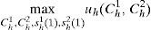
- (i)
The budget restrictions given by,
with multipliers λh(0), andwith multipliers, λh(ω) - (ii)
The portfolio constraint as expressed by,
with multiplier, υ - (iii)
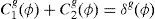
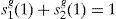
And the market clearing conditions


All technical steps taken to solve the model appear in Appendix A. We basically follow the two step approach employed by BCLP (2008). The critical feature of this approach is to ignore the complementary slackness condition associated with the portfolio constraint until the very end of the analysis, which is known as “tailoring” the constraint. According to BCLP (2008), this approach can be used for analyzing many second best problems like the present analysis of the effects of introducing a portfolio constraint on the set of financial equilibria. By specifying this constraint in sufficiently rich parametric form, one can first consider just the effects of the modifications of first-order conditions and, subsequently in the second step, the tailoring of parameters in order to also satisfy complementary slackness conditions.
Additionally, the technical steps employ the following modified variables:

It should be noted that we can use these transformation units because the intrinsic uncertainty represented by Jhg(ϕ) is not relevant to the fundamental structure of the system of equations defining the equilibrium in our model. Our assumptions on Jhg(ϕ) allow us to work with constant jhg(ϕ) between states of the world, facilitating the analysis. Hence it can be labeled simply as jhg. In addition, variations in jhg are only due to variations in Jhg(ϕ). Note also that if Jhg(ϕ)<0 and |Jhg(ϕ)|
A key aspect of the methodology is the introduction of the households’ “stochastic weights”:

It is useful to conduct the analysis in terms of these variables rather than, in particular, spot goods prices. Since this is a model with real assets (stock payoffs are specified in terms of goods), and there are three spots, there are also three possible price normalizations. For this reason we adopt the normalization η1(ϕ)=1, so that we can simply write η2(ϕ)=η(ϕ), for all ϕ. None of the results depends on this choice. As pointed out by BCLP (2008), the quantities ηh(ϕ) can be interpreted as the weights of the households’ utilities in an auxiliary social planner's problem, even if they are not Pareto efficient. Note also that Pareto efficiency of the equilibrium allocation requires that η(ϕ) be a constant weight across all ϕ.
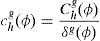
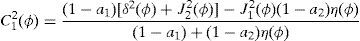
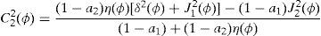
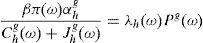
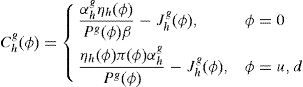
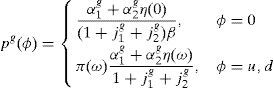
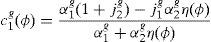
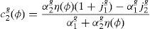
2.3Equilibrium in consumer and financial marketsIn this section we present the equilibrium expressions for the main endogenous variables for the model with the generalized logarithmic utility function; that is to say, consumption, spot good prices and stock prices.Proposition 1 The consumption allocations, the spot good prices and the stock prices are given by,


See Appendix A.8□
It is important to point out that, when Jhg(ϕ)>0, the utility function will not guarantee non-negative consumption. In Appendix A we show that the equilibrium consumption is positive if and only if:

Equivalently (taking into account expression (6c)


Note that the expressions in Proposition 1 depend on η(0), η(u) and η(d). Then, to solve the model we need to know the value of these stochastic weights. We deal with this issue in section 2.5.
In the following result, we obtain the expressions for optimal portfolio holdings of the households:Proposition 2 When the households have a generalized logarithmic utility function, their optimal portfolio holdings in any inefficient equilibrium, η(u)≠η(d), are given by


See Appendix A.□
Note that the expressions for the optimal portfolio holdings in any inefficient equilibrium of Proposition 2 can be generalized to,
where hˆ represents the other household.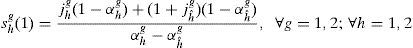
We now provide some remarks about shg(1). First of all, note that shg(1) is decreasing in the marginal propensity to consume of the household h, αhg. Namely, the greater is his propensity to consume, the more he prefers consuming goods than acquiring stocks. On the other hand, shg(1) is increasing in Jhg (recall that variations in jhg are only due to variations in Jhg) if and only if αhg>αhˆg; otherwise it is decreasing.9 This can be explained by noting that, when Jhˆg increases, the household hˆ tries to compensate his lower αhˆg in the utility function with a greater consumption, which means acquiring less assets.
Next note that when Jhg(ϕ)≥0, ∀h=1,2, the household with the lowest marginal propensity to consume will take the short position. However, when Jhg(ϕ)<0 this will not always be true, since there are examples in which both households acquire positive quantities of the stocks. Otherwise, when Jhg(ϕ)≤0, shg(1) does not depend on the state of the economy. To see this, notice that when Jhg(ϕ)>0, the parameter Jhg of one of the households must satisfy (10) and (11) (or equivalently, jhg must satisfy (8) and (9)). Then, the parameter jhg of one of the households will fall within a range whose boundaries depend on η(ϕ). Therefore, shg(1) must depend on the state of the economy.
Finally, let shg(1)CD=(1−αhˆg/(αhg−αhˆg)) be the expression for the optimal portfolio holdings in any inefficient equilibrium in the BCLP (2008) framework. Then, shg(1)=shg(1)CD if and only if Jhg=−(1−αhˆg/(1−αhg))Jhˆg. Note that Jhˆg can be either zero (and then Jhg=0, ∀h=1,2), or different from zero. In this later case, one household has J>0 and the other has J<0, but their optimal portfolio holdings in any inefficient equilibrium are the same as when they have J=0.
2.4The portfolio constraintWe consider next a constraint imposed on the fraction of wealth household 2 is permitted to invest in the second stock:
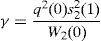
where household 2 initial wealth is defined as the value of his portfolio,and γ>0 is endogenously determined. It can be shown that that,10where2.5Multiplicity of equilibrium with portfolio constraints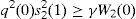


Next we find the value of the stochastic weights. In Appendix A we show that,
where Γ is given by the long expression (A30) reported in Appendix A, and η(u) and η(d) solve the following system,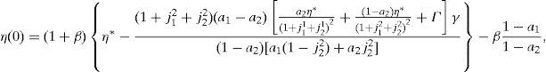
Given these expressions, we can now state the following result,Proposition 3 With complete markets and generalized logarithmic utility, there is a multiplicity of inefficient equilibria in the economy in which the portfolio constraint is binding. Without the portfolio constraint, the equilibrium is unique and Pareto efficient. When η(0)=η*, (20) has a unique solution: η(u)=η(d)=η*. In this case the portfolio constraint is not binding and the equilibrium is unique and Pareto efficient. But for some values of γ, it is necessarily the case that η(0)≠η*. Then the system of equations (20) is quadratic and admits two solutions. In this case, as desired, there exist two inefficient equilibrium points in which the portfolio constraint is binding.□
In this section we add a new state of the world, ω=m (“middle”), so that in period 1, ω=u, m, d (and ϕ=0, u, m, d) occurring with probabilities π(ω). The rest of the economic environment remains the same, and in particular, there are still two stocks–one fewer than there is states of the world.
The households’ portfolio holdings in Proposition 2 are the portfolio holdings supporting equilibrium in the economy with incomplete markets. And the expressions for η*, γ and η(0) are the same as those for complete markets. However, η(u), η(m) and η(d) solve now the following system,
The proof appears in Appendix B.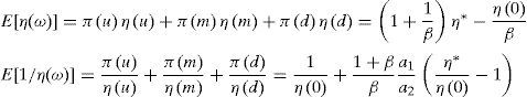
Similarly to the previous case, when η(0)=η*, (21) has a unique solution: η(u)=η(m)=η(d)=η*. Thus, the equilibrium is unique and Pareto efficient, and the portfolio constraint is not binding. But when, for some values of γ, η(0)≠η*, the system of equations (21) has a continuum of solutions. Hence, there is a continuum of inefficient equilibria in which the portfolio constraint is binding. We can therefore state the following proposition,Proposition 4 With incomplete markets and generalized logarithmic utility, there is a continuum of inefficient equilibria in which the portfolio constraint is binding. Without the portfolio constraint, the equilibrium is unique and Pareto efficient. See Appendix B.□
We can conclude that the multiplicity of equilibria obtained by BCLP (2008) is robust to a generalized specification of the log-linear utility function. The fact that multiplicity of equilibria under portfolio constraints is a valid result under decreasing, constant, and increasing relative risk aversion is an important result to better understand financial market prices. This is a first extension of BCLP model, but much more research needs to be done to fully investigate (and understand) the potential consequences of portfolio constraints on asset allocation and asset pricing.
Alex Barrachina and Amparo Urbano acknowledge financial support from the Ministry of Science and Technology and the European Feder Funds under projects SEJ2007-66581 and ECO-2010-20584. Gonzalo Rubio acknowledges financial support from Ministry of Science and Innovation grant ECO2008-03058/ECON and CEU-UCH/Banco de Santander Copernicus 4/2011, and Amparo Urbano and Gonzalo Rubio thank the Prometeo Programme of the Generalitat Valenciana for financial support under projects PROMETEO/2009/068 and PROMETEO/2008/106 respectively.
The basic system of EFEs describing the financial equilibrium consists of the usual first-order conditions (FOCs), no-arbitrage conditions (NACs), and spot budget constraints (SBCs) for both households, together with the market clearing conditions (MCCs) for goods and stocks.
FOC:
NAC:
where σ=0,g=1υ,g=2SBC:
MCC:
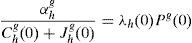


Rewriting the FOCs given by (A1) and (A2) and using the definition of stochastic weight given by (7) we have,
Solving for Pg(0) in (A9), summing over h and bearing in mind that now η1(ϕ)=1 and η2(ϕ)=η(ϕ),
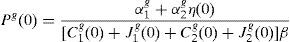
Replacing (A10) in expression (6a) and taking into account expressions (6b) and (6c),
Proceeding the same way for Pg(ω) in (A9), we obtain
The last two expressions are the equilibrium prices of the goods:
Dividing the expression (A9) by δg(ϕ), taking into account expressions (6a)–(6c) and replacing (A11) in the resultant expression, we obtain the equilibrium consumption of household 1:
From the market clearing condition (A7) and expression (6b), we have that c1g(ϕ)+c2g(ϕ)=1. Hence, the equilibrium consumption of household 2 is,
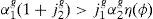
Next, note that when Jhg(ϕ)>0, the utility function by itself does not guard against negative consumption. It is easy to show that (A12) is positive if and only if α1g(1+j2g)>j1gα2gη(ϕ), and (A13) is positive if and only if α1gj2g<α2gη(ϕ)(1+j1g). Then the parameter jhg of one of the households must fall within a range whose boundaries depend on η(ϕ).
Rewriting the period one spot budget constraint (SBC) of the household 1 given by (A6) taking into account the expressions (6a) and (6b),

Replacing (A11), (A12) and (A13) in the last expression and taking into account that α11+α12=a1+(1−a1)=1, we have,
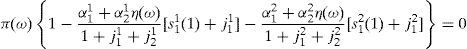
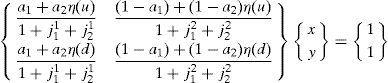
Equivalently,
where x=s11(1)+j11 and y=s12(1)+j12.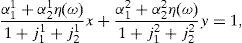
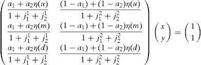
Note that when η(u)≠η(d); i.e. when an inefficient equilibrium occurs, (A14) is a system of two equations with two unknowns:
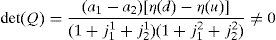
The determinant of the matrix Q above is given by
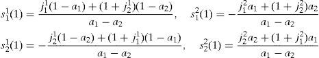
Solving the system, we obtain the optimal portfolio holdings of the households in any inefficient equilibrium:
So, clearly, when the stochastic weights are identical across the two states of the world η(u)=η(d), the determinant of Q is zero and the matrix is not invertible. Hence, one of the stocks is redundant, and the portfolio holdings of households in each stock are indeterminate.
If η(u)=η(d)=k>0, the expression (A14) becomes,
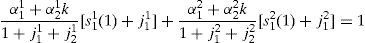
Solving for s11(1) we have,
where ξ=(1+j11+j21/(1+j12+j22)).
According to the market clearing condition (A8),

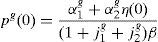
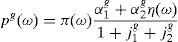
Next, we rewrite the no-arbitrage condition (NAC) of household 1, given by (A3), taking into account expression (6a), and bearing in mind that λ1(ϕ)=β, since η1(ϕ)=1. Solving for qg(0) in the resultant expression, we have,
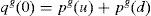
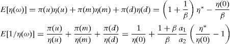
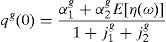
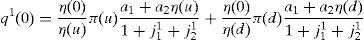
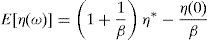
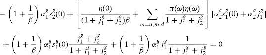
Replacing (A11) in (A16), and defining E[η(ω)]=(π(u)η(u))+(π(d)η(d)), we obtain the equilibrium prices of the financial assets:
It is now clear that, with the exception of the optimal portfolio holdings, the equilibrium results of the model depend on η(ϕ). We obtain the value for these stochastic weights from the RFEs. The RFEs are three equations that can be obtained from the EFEs.
- (i)
The first RFE:
Rewriting SBC of the household 1 given by (A5) and (A6) taking into account the expressions (6a) and (6b),
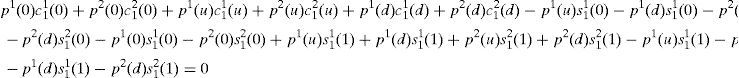
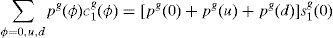
adding these three expressions,and replacing in this resultant expression the equilibrium prices of the financial assets given by (A17),we obtain,that we summarize inReplacing (A11) and (A12) in the last expression, then simplifying (in particular, using the fact that s1g0+s2g0=1) and multiplying the resulting equation by -1, we obtain the first RFE (see the system of the three RFEs below).
- (ii)
The second and third RFEs:
Rewriting the NAC of household 2, given by (A4), taking into account the expression (6a),
Solving for q1(0) in (A18), replacing (A11) into the resultant expression, and taking into account the definition of stochastic weight given by (7), we have,
Solving for q2(0) in (A19) and proceeding the same way, we have,
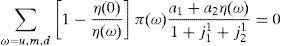
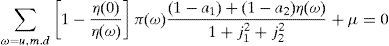
Equating the expressions (A20) and (A21) to the expression we obtained for the equilibrium prices of the financial assets, given by (A17), and defining μ=(υη(0)/β), we obtain the second and third RFEs (see the system of the three RFEs below).
- (iii)
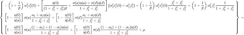
The system of the three RFEs:
The three RFEs form the following system (SY hereafter).
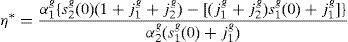
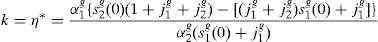
When η(ϕ)=k, ∀ϕ; i.e. in a Pareto efficient situation, the second EFR holds, the third equation holds if and only if μ=0, and from the first RFE we can obtain the expression for k:
Therefore, when η(ϕ)=η*, μ=0. This implies that there is a unique Pareto efficient equilibrium, and in this equilibrium the portfolio constraint is not binding. As BCLP (2008) do, because the existence of η*>0 is so central to our analysis of SY, we assume that (A22) obtains.


Consider the specific portfolio constraint
where W2(0) is the value of the initial portfolio of the household 2: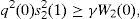

When μ>0 this constraint is binding and (assuming that W2(0)>0) we can solve for γ in (A23),
But first, we rewrite (A24) taking into account expression (6a),

Replacing (A11) and (A17) into the last expression, we have,

Next, solving for E[η(ω)] in the first RFE, we have,
Equivalently,

Replacing (A28) into (A26), we obtain,
where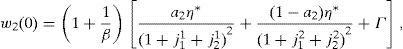
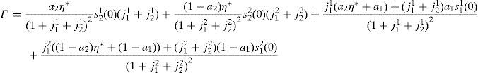
Now replacing the equilibrium expression for s22(1) given in (A15), and the expressions (A17) and (A29) into (A25), we obtain
where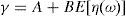


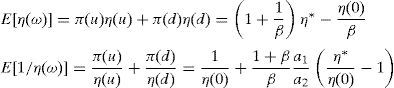
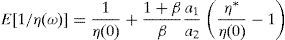
Solving for E[η(ω)] in (A31) and replacing the resulting expression into (A28), we obtain

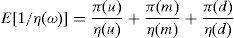
Defining E[1/η(ω)]=(π(u)/η(u))+(π(d)/η(d)) and from the second RFE, we have,
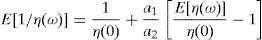
Replacing (A27) into the last expression, we obtain,
Hence, we must find the values of η(u) and η(d) that solve the system defined by (A27) and (A33):
□
The procedure in the incomplete markets case is the same as in Appendix A, except that now we must assume three (period-1) spot budget constraints, corresponding to ω=u, m, d. Accordingly, the number of stochastic weights increases from 3 to 4 (one for period 0 and one for each of three possible states ω). In this case, the equation determining terminal portfolio holdings, which is equivalent to (A14), takes the form,
It is easy to verify that the households’ portfolio holdings reported in Proposition 2 are the portfolio holdings supporting equilibrium in the economy with incomplete markets.
Moreover, as before, the logic of the reduction of the EFEs leads to just three RFEs,
The expressions for η*, γ and η(0) are the same as in the complete markets case, and they are given by (A22), (A31) and (A32) respectively. However, we have to be careful now because,

Hence, when the financial markets are incomplete, we must find the values of η(u), η(m) and η(d) that solve the following system:
□