


Recent literature has proved that many classical very important pricing models of Financial Economics (Black and Scholes, Heston, etc.) and risk measures (VaR, CVaR, etc.) may lead to “pathological meaningless situations”, since there exist sequences of portfolios whose negative risk and positive expected return are unbounded. Such a sequence of strategies will be called “good deal”.
This paper focuses on a discrete time arbitrage-free and complete pricing model and goes beyond existence properties. It deals with the effective construction of good deals, i.e., sequences (ym)m=1∞ of portfolios such that
Risk measurement is becoming more and more important in financial literature. A clear proof is the growing interest of many authors about the formal properties that a risk measure must satisfy. Indeed, among other interesting contributions, Artzner et al. (1999) introduced the Coherent Measures of Risk, Goovaerts et al. (2004) introduced the Consistent Risk Measures, Rockafellar et al. (2006) defined the Expectation Bounded Risk Measures, Balbás et al. (2009) studied the Adapted Risk Measures, Aumann and Serrano (2008) and Bali et al. (2011) defined Indexes of Riskiness, and Cerreia-Vioglio et al. (2011) defined the Cash-Sub-Additive and Quasi-Convex Risk Measures. All these measures are more and more used by researchers, practitioners, regulators and supervisors.
Many authors have revisited the most important classical actuarial and financial problems by drawing on the risk measures above. With respect to the Portfolio Choice Problem, interesting contributions may be found in Stoyanov et al. (2007), Rockafellar et al. (2007), Miller and Ruszczynski (2008), Zakamouline and Koekebbaker (2009), and Balbás et al. (2010a), among others. Usually, authors attempt to maximize a generalized Sharpe ratio or deal with a vector optimization problem involving the expected return and a (maybe vector) risk measure. In this sense, they extend the Markowitz approach, but the role of the standard deviation is played by a more complex risk measure.
A second recent line of research focuses on the notion of “Good Deal” (GD), introduced in Cochrane and Saa-Requejo (2000). Mainly, a GD is an investment strategy providing traders with a “very high Sharpe ratio”, in comparison with the Market Portfolio. In the paper of Cochrane and Saa-Requejo the risk was measured with the standard deviation, and the absence of GD was imposed in an arbitrage-free incomplete pricing model so as to price non-reachable pay-offs. Unreachable pay-offs are priced in such a manner that buyers (sellers) cannot create a GD with huge Sharpe ratios provoked by low (high) bid (ask) prices. In practice, the absence of GD generates bid/ask spreads (or good deal bounds) much lower than those implied by arbitrage arguments. Consequently, many researchers have extended the discussion and dealt with GD-linked pricing methods, obtaining GD bounds and hedging strategies much more realistic and empirically relevant than the classical arbitrage-linked bounds and hedging strategies. Moreover, this line of research has been generalized for risk measures beyond the standard deviation (among others, Staum, 2004, or Arai, 2011, present further studies about all of these topics).
When portfolio choice problems do not focus on the standard deviation and minimize other risk measures, it is not guaranteed that the problem will be bounded. In particular, Balbás et al. (2010a) have shown that every pricing model whose Stochastic Discount Factor (SDF) follows a log-normal or a heavier-tailed distribution (Black and Scholes, Heston, etc.) will generate meaningless situations when combined with every coherent and expectation bounded risk measure. Indeed, for every pricing model and risk measure as above, there are sequences of portfolios whose risk tends to minus infinity or remains bounded and whose expected return tends to plus infinity (risk=−∞, return=+∞ or risk≤CONSTANT, return=+∞). The analysis of Balbás et al. (2010a) has been extended in Balbás et al. (2010b), where the authors present explicit constructions of the sequences above for the Conditional Value at Risk (CVaR) with an arbitrary level of confidence and the Black and Scholes model. Balbás et al. (2010b) use the expression GD to indicate such a sequence. Actually, according to the results above, the generalized Sharpe ratio “Return/CVaR” may tend to infinity, and therefore it will outperform the Market Portfolio generalized Sharpe ratio. Since the ratio may become as close as desired to infinity, the notion of GD in Balbás et al. (2010b) is obviously more restrictive than it is in the papers above (Cochrane and Saa-Requejo, 2000; Staum, 2004; Arai, 2011). Surprisingly, despite the fact that the absence of GD may be useful to price in incomplete models, complete ones such Black and Scholes are not GD-free for general risk measures beyond the standard deviation. This paradox implies that the explicit computation of GD in complete models becomes a critical point, since it may help to study what is the economic/financial meaning of the GD-absence assumption.
This paper adopts the notion of GD of Balbás et al. (2010b) and deals with the Value at Risk (VaR) and the CVaR so as to present effective GD constructions for every discrete time arbitrage-free and complete pricing model such that the existence of GD holds. In other words, for an arbitrary (discrete) pricing model, if there are sequences (ym)m=1∞ of pay-offs such that
holds, then they can be computed by the algorithms that we will present. Moreover, as a second contribution, we will provide a sensitivity analysis, i.e., we will measure the effect on the GD of estimation errors or dynamic evolutions of some key variables such as the SDF of the pricing model.
We have selected VaR and CVaR because they are becoming more and more popular for researchers, practitioners, regulators and supervisors, and they are also playing an important role in international regulations such as Basel II and III.1 We have selected a discrete time framework because it significantly simplifies the mathematical exposition of the paper. Moreover, since most of the continuous time pricing models have an appropriate discrete time approximation, it seems that the provided algorithms may be quite useful to traders in practice. Needless to say that return/risk ratios are crucial in order to rank the effectiveness of portfolio managers.
The article's outline is as follows. Section 2 will present our notations and a important background that will be applied. We will deal with the framework of Balbás et al. (2010b), so some further details may be found in that paper. There are no contributions in this section, but it has been included for expositional simplicity. Section 3 is the most important one of the paper. In particular, Theorems 4 and 5 will yield closed formulas providing us with a GD in a very general discrete time setting. They are crucial to develop two new algorithms in Remarks 3 and 4. Four numerical experiments with the popular binomial pricing model will be summarized in Section 4. They mainly have illustrative purposes, though the fourth one involves real market data related to the American index SP500 during the year 2011. We did not implement any exhaustive empirical test, but, for the index and year above, the GD practical performance was quite satisfactory. Besides, the third numerical example will show that the algorithms are flexible enough, in the sense that they may dynamically incorporate market evolutions that the pricing model does not predict (modifications in volatilities, interest rates, etc.). Nevertheless, since it may be also interesting to anticipate these changes and have initial information about their possible effect on the GD, Section 5 is devoted to measuring the sensitivity of our solutions with respect to them, as well as the sensitivity with respect to possible measurement errors. Theorem 6 gives a general formula when the GD price, the random final wealth of the manager, and/or the pricing model (the SDF) are modified. Finally, Section 6 presents the most important conclusions of the paper.
2Preliminaries, notations and theoretical backgroundConsider the probability space (Ω,F,IP) composed of a finite set of “states of the world” Ω, the σ-algebra F containing all the subsets of Ω, and the probability measure IP whose support is Ω. Consider also a time interval [0, T], a finite subset T⊂[0,T] of trading dates containing 0 and T, and a filtration (Ft)t∈T providing the arrival of information such that F0={∅,Ω} and FT=F. As usual, there are several available securities whose price processes are adapted to (Ft)t∈T. Suppose that the market is complete, i.e., every final pay-off (or F-measurable random variable) y∈IRΩ may be reached by the price process (St)t∈T of a self-financing portfolio, in the sense that the equality ST=y holds. Then, S0 may be interpreted as the initial (at t=0) price Π(y) of the pay-off y, and we will assume that the pricing rule Π:IRΩ⟶IR is linear (i.e., there are no frictions).
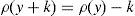
The completeness of the pricing model implies the existence of a risk-free asset. Thus, if rf≥0 is the risk-free rate, equality
must hold for every k∈IR. Besides, according to the Riesz Representation Theorem, there exists a unique zπ∈IRΩ such thatfor every y∈IRΩ, IE() representing the mathematical expectation. Moreover, to prevent the existence of arbitrage, the strict inequalitymust hold. zπ is usually called “Stochastic Discount Factor” (SDF, see Duffie, 1988, for further details).
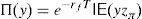

Expressions (1) and (2) imply that ke−rfT=Π(k)=e−rfTkIE(zπ), which leads to

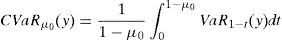
We will deal with two risk measures in this paper: The Value at Risk (VaRμ0) and the Conditional Value at Risk (CVaRμ0), with μ0∈(0, 1) being the confidence level. They are given by (Rockafellar et al., 2006)
andfor every y∈IRΩ. Moreover, if the CVaRμ0 sub-gradient is defined bythenholds for every y∈IRΩ (Rockafellar et al., 2006). Finally, if ρ=VaRμ0 or ρ=CVaRμ0 for some level of confidence 0<μ0<1, all of the properties below hold:for every y∈IRΩ,for every y∈IRΩ and k∈IR,for every y∈IRΩ and α>0,for every y1, y2∈IRΩ,for every y∈IRΩ, andfor every y1, y2∈IRΩ with y1≤y2.2
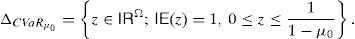


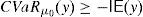

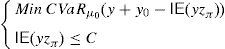
Suppose that the random variable y0∈IRΩ represents a trader's final (at T) wealth (or pay-off). The risk level is given by ρ(y0). Then ρ(y0) may be an adequate final value (at T) of the capital requirement. Indeed, (8) leads to
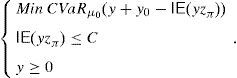
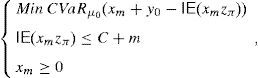
and the risk will vanish if the additional amount ρ(y0)e−rfT is invested in the risk-free security. Nevertheless, Balbás et al. (2010b) have proved that this investment in the risk-free security may be outperformed by alternative hedging strategies y∈IRΩ, in the sense that the current price of y is still ρ(y0)e−rfT but the global risk ρ(y0+y) is negative. More accurately, these authors consider the pay-off y∈IRΩ added by the trader to his pay-off y0∈IRΩ, they suppose thatgives (the value at T of) the highest amount of money devoted to reducing the risk level,3 and they finally propose the following optimization problems so as to select y:andProblem (15) involves the global risk CVaRμ0(y+y0−IE(yzπ)) that the trader is facing, so it has to incorporate the value IE(yzπ) of the added portfolio, that will have to be paid and will reduce the trader's wealth. Constraint y≥0 may be indicating the presence of short-selling restrictions. Since we are minimizing risk, one can consider that short sales must be allowed if they do not make the riskiness increase, so Problem (16) also makes sense. In fact, the optimal risk in (16) will never be higher than the optimal risk in (15), since every (15)-feasible solution is also (16)-feasible.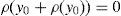

Since y=0 satisfies the constraints of (15) and (16) both problems are feasible. However, the paper above presents examples illustrating that (16) may be unbounded, i.e., there may be sequences (yn)n=1∞ of pay-offs such that CVaRμ0(yn+y0−IE(yzπ))→−∞. Furthermore, as we will prove in Proposition 1 below, if the existence of this sequence holds then it provides us with returns converging to +∞. Henceforth, these sequences will be called good deals (GD).
Proposition 1 If the sequence(yn)n=1∞satisfiesLimn→∞CVaRμ0(yn+y0−IE(ynzπ))=−∞, then


Following Balbás et al. (2010b), the solution y* of (15), if it exists, will be called “shadow riskless asset” (SRA).
The rest of this section is devoted to summarizing some findings of Balbás et al. (2010b) that will apply henceforth. In particular, (6) implies that
is the dual of (15), λ∈IR and z∈ΔCVaRμ0 being the decision variables.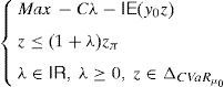
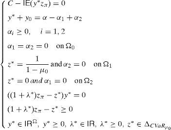
Theorem 2 Suppose thatIPzπ>11−μ0>0.4Then: Problem(16)is unbounded, i.e., there are good deals. (15) and (17)are bounded and solvable, and there is no duality gap (i.e., both problems attain their common optimal value). If y*∈IRΩand (λ*, z*)∈IR×IRΩ, then they solve(15) and (17)if and only if there exist α∈IR, α1, α2∈IRΩand a disjoint partition Ω=Ω0∪Ω1∪Ω2such that the following Karush–Kuhn–Tucker conditions
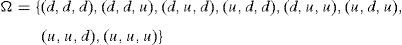
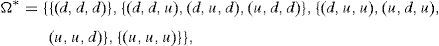
Conditions (18) may be complex in practical applications. Thus, let us simplify them. We will look for the optimal solution of (15) among the non-path-dependent European style derivatives with maturity at T and whose underlying asset is y0. The obvious implication is that the final pay-off of every non-path-dependent European style derivative is a function of y0, so ω∈Ω is not so important and only y0ω matters. The set of states on nature Ω may be replaced by a new set Ω*⊂Ω only distinguishing the final values of y0, and Π may be replaced by its restriction too. Illustrative examples will be given in Section 4. Proposition 1 and Theorem 2 still applies if Ω* plays the role of Ω. Clearly, once the solution y* of (15) has been obtained, the self-financing trading strategy leading to the pay-off y* will have to be constructed in the initial setting Ω,F,IP. Once again, the examples of Section 4 will clarify it.
Hence, without loss of generality we can consider that
and y0ω increases as so does ω∈Ω*. We will also assume thatand zπω decreases as so does ω∈Ω*. Once again, Section 4 will clarify that zπ usually decreases in practical applications such that y0 increases.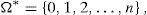
Summarizing we have:
Assumption 1 Ω* is given by (19), y0 is a strictly increasing function of ω∈Ω*, zπ is a strictly decreasing function of ω∈Ω*, and (20) holds.5 □
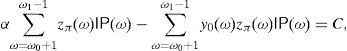
Remark 1 Under the conditions above, Theorem 2a implies the existence of good deals, while Theorem 2b implies the existence of both a dual solution λ*,z* and a SRA y* which is not risk-free. Furthermore, Theorem 2b also leads to both the equality

Let us give several properties that will allow us to solve (15) and (16).6 First of all, though (15) and (16) are not linear, Problem (17) is linear, and it can be solved by standard well-known methods. Thus we can assume that (λ*, z*) is known.
Theorem 3 z*is decreasing, i.e., ifω,ω˜∈Ω*,ω<ω˜, thenz*(ω)≥z*(ω˜).
Proof Suppose that z*(ω)

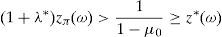
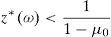
Remark 2 Expression (20) implies the existence of ω∈Ω* with zπ(ω)>11−μ0. Since λ*>0 (see (22)), we have that
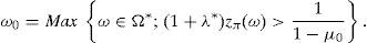
Similarly, if IP(z*>0)<1, there exists
and we will define ω1=n+1 if IP(z*>0)=1. □
Next let us show that 0,1,…,ω0 and ω1,…,n are disjoint, along with the expression of y* and z* in these subsets of Ω*.
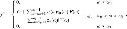
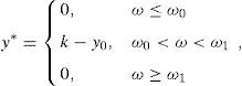
Theorem 4 IfIPz*>0<1then
y*(ω)=0 for every ω≤ω0.
IfIP(z*>0)<1 then y*(ω)=0 for every ω≥ω1.
ω0<n, and ω0+1<ω1ifIP(z*>0)<1.
z*(ω)=11−μ0for every ω≤ω0.
Proof
Statement (a) implies that z*(ω)=0. Expression (3), along with the eighth and ninth conditions in (18), show that y*(ω)=0. Similar arguments show that ω0<n.
ω0+1≥ω1 and Statements (b) and (c) would lead to y*=0, in contradiction with (21) and (14).
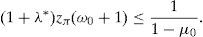
Theorems 3 and (5) imply that one only has to prove z*(ω0)=11−μ0. If z*(ω0)<11−μ0 then ω0∈Ω0 in (18) due to Statement (d). Hence, according to Statement (b),
On the other hand, ω0+1∉Ω2 in (18) due to Statement (d). Hence,We have a contradiction because y0 is strictly increasing.

The SRA y* is already known in {0, 1, …, ω0} and {ω1, …, n}, so let us compute y* within the interval ω0<ω<ω1.
Theorem 5
If(26)is a strict inequality then
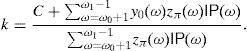
If(26)becomes a equality then there existα≥α˜>0such that
Moreover,andα˜=y0(ω0+1)ifz*(ω0+1)<11−μ0. Finally, ifz*(ω0+1)=11−μ0then0<α˜≤αmay be arbitrary as far as y*≥0 and the eighth condition in(18) and (29)hold.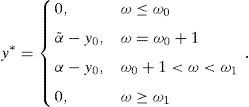
Proof It trivially follows from (23). If (26) is a strict inequality then

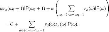
If (26) becomes a equality then (30) and (31) still hold for ω0+1≤ω≤ω1−1 and ω0+1<ω. As in (b), y*=α−y0 for ω0+1≤ω≤ω1−1 and ω0+1<ω. As in (b), z*(ω)>0 for ω0+1≤ω≤ω1−1, so ω0+1 does not belong to the set Ω2 of (18) and α2(ω0+1)=0. Whence
Eq. (28) trivially follows if one takes α˜=α−α1(ω0+1), which is strictly positive because otherwise y*(ω0+1) would be strictly negative, in contradiction with the constraints of (15). Furthermore, (29) trivially follows from (21), α˜=y0(ω0+1) if z*(ω0+1)<1/(1−μ0) due to the eighth condition in (18), and finally, we only must guarantee the fulfillment of (18) if z*(ω0+1)=1/(1−μ0).
Remark 3 (General algorithm to build the SRA). Theorem 5 above allows us to find y* in practice. The steps are: Solve the linear programming problem (17) by standard methods (for instance, the simplex method). Theorem 2b guarantees that it is bounded and solvable. We have the dual solution (λ*, z*). Compute ω0 and ω1 according to (23) and (24). Take ω1=n+1 if IP(z*>0)=1. Take y*(ω)=0 for ω≤ω0. If IP(z*>0)<1 then take y*(ω)=0 for every ω≥ω1 (Theorem 4). Verify whether (26) is a equality or a strict inequality.
If (26) were a equality then take y* as in (28) and (29) (Theorem 5).
Remark 4 (General algorithm to build a GD). Let us assume that there are no short selling restrictions, i.e., let us deal with (16) rather than (15). Theorem 2a shows that there is a GD. In other words, one can construct sequences of portfolios whose

Consider m∈IN, along with an approximation of (16) given by Problem
Then, due to (4), it is easy to see that the change of variable xm=y+m leads towhich is a new problem analogous to (15). Thus, (33) is bounded and achieves its optimal value (Theorem 2b). Consider the sequence (ym*)m=1∞=(xm*−m)m=1∞ of solutions of (33), (xm*)m=1∞ denoting the solutions of (34). It is easy to see that (ym*)m=1∞ is a GD. Furthermore, every xm* may be computed with the algorithm of Remark 3. Notice that (4) and (8) lead toand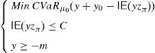


Since the limit equality
is obviously unreachable, in practice one can proceed as follows: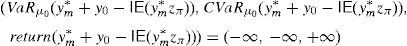
- Step a
Fix a desired finite level (A, B, C) for (VaRμ0,CVaRμ0,return).
- Step b
Apply the algorithm of Remark 3 in order to compute ym* for several values of m∈IN, and then stop once VaRμ0≤A, CVaRμ0≤B, and return≥C.
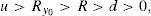
Assumption 1 usually holds in practice. For instance, suppose that the random pay-off y0 satisfies the binomial probability distribution, i.e., the price process with final (at T) pay-off y0 is given by the binomial model with n periods. The set Ω* of (19) will indicate the number of growths of this price process between 0 and T, and therefore
for every ω=0, 1, 2, …, n, W>0 denoting the price of the portfolio at t=0, and u>1 and d<1 denoting the usual factors affecting this portfolio price between two consecutive trading dates. y0 is obviously a increasing function of ω. We can also assume that zπ(ω) decreases as ω∈Ω increases since this is the usual situation if the market is risk adverse. Indeed, if ∇(t) represents the time length between consecutive trading dates, and R=erf∇(t)∈(d, u) represents the capitalization factor of the risk-free asset, thenRy0 denoting the expected return of y0 between two consecutive trading dates. Obviously, since y0 is risky, in an arbitrage-free risk adverse world we have thatand zπ is decreasing.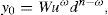
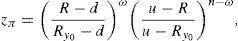
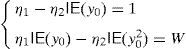
Beyond the binomial model, Assumption 1 is usually fulfilled too. Indeed, in a general risk adverse framework, if we assume that ω=0, 1, 2, …, n is the number of growths of the price process leading to the pay-off y0, and this pay-off is efficient in a (return, standard_deviation) setting, then there exists a couple of strictly positive real numbers η1 and η2 such that
and therefore zπ is strictly decreasing if y0 is strictly increasing. In practice, η1 and η2 may be easily computed from (4) and taking into account that W is the current price of the self-financing portfolio with pay-off y0. Thus, Systemmust hold.
Dealing again with the binomial model, let us present four examples of the two given algorithms (Remarks 3 and 4). Examples 1–3 are just presented for illustrative purposes, whereas Example 4 deals with real market data.7
Example 1 Consider that the manager's portfolio price process is given by the binomial model composed of three periods (four trading dates denoted by 0, ∇(t), 2∇(t), and 3∇(t), for some ∇(t)) such that R=1.01, d=0.5 and u=2. Suppose that the initial (at t=0) portfolio price is W=200. The binomial tree below indicates the price process we must deal with


Example 2 Once we know the SDA of Example 1, let us build the GD. According to Remark 4, we can solve (33) and (34) for C=100 and m=1000, 2000, 3000, …. If we select m=30,000, then the solution of (34) leads to the final pay-off


Example 3 Next let us assume that the parameters of the binomial model may be dynamic. For instance, in practice, the binomial model is an approximation of the Black and Scholes model. Thus, the volatility σ of the process may be dynamically estimated, and therefore


In order to illustrate the method, consider again the parameters of Example 1. Suppose that after one period the underlying asset price becomes 400 (see (39)), u=4 and d=0.25. Then, prices and deltas of the SRA in (40) must me modified according to the new trees
Optimal risk levels have become different too due to the evolution of u and d. The new values are VaR0,7(y*+y0−IE(y*zπ))=−602.31 and CVaR0,7(y*+y0−IE(y*zπ))=−181.64. Obviously, if one period later the parameters become different again, the right hand side of the trees above will have to be modified for the second time. □
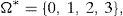
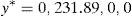
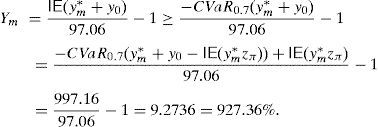
Example 4 Let us construct a SRA for the SP500 American index. We have selected the year 2011 and the period [0, T] =[March_14th,March_18th] because the return of the SRA was very large, but, in general, our empirical test affecting the SP500 index and the whole year 2011 reveals that the SRA may generate very acceptable returns. On March 14th, 2011, the SP500 index value was 1296.39, and the VIX index value was 21.13%. Suppose that VIX index may be interpreted as a predictor of the SP500 volatility. We will construct the SRA with current price 100 and maturity T=[March, 18th, 2011], by dealing with a binomial model such that ∇(t) equals one day (or 1/260 years), and the risk-free rate vanishes. Parameters u and d are given by (42) and (43). Obviously, there are four periods, so Ω*={0, 1, 2, 3, 4}. If μ0=70% and we assume that the SP500 annual expected return equals 20%, then the algorithm of Remark 3 leads to the SRA

Example 3 has illustrated that changes in the parameters of the pricing model within the period (0, T) may be incorporated to the algorithms. Nevertheless, it may be interesting to have a previous estimation about the effect that those changes could provoke on the optimal risk value CVaRμ0(y*+y0−IE(y*zπ)).
This section is devoted to quantifying the effect on CVaRμ0(y*+y0−IE(y*zπ)) of measurement errors and changes in the pricing model. To this purpose we will draw on the classical “Envelope Theorem” of Mathematical Programming. Mainly, this theorem states that the optimal value sensitivity (partial derivative) with respect to every involved parameter equals a partial derivative of the Lagrangian Function.
Consider 0<μ0<1 and Problem (15) for a variable C>0 belonging to an open set of IR and variables y0 and zπ belonging to open sets of IRΩ. Suppose that IP(zπ>1/(1−μ0))>0 holds for every feasible zπ. Theorem 2 guarantees the existence of solution for (15). Define CVaRμ0*(C,y0,zπ) as the optimal value of (15), that depends on (C, y0, zπ).
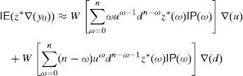
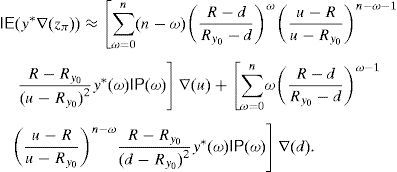
Theorem 6 FunctionCVaRμ0*is Fréchet differentiable and

Proof The Envelope Theorem of Mathematical Programming implies that CVaRμ0* is Fréchet differentiable if so is the Lagrangian Function at the primal,dual solution, and both differentials coincide. The Lagrangian Function of (15) is (see Balbás et al., 2010c, for a general Lagrangian Function of optimization problems involving risk measures)

Remark 5 Theorem 6 enables us to give an approximation of the optimal risk level variation ∇(CVaRμ0*) with respect to modifications of the parameters. In particular,

Remark 6 In the particular case of the binomial model, if u and d are modified, (35) and (36) obviously lead to
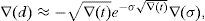
Therefore, (44)–(46) will give the variation ∇(CVaRμ0*) of the optimal risk level with respect to the parameters u and d. Similarly, bearing in mind (35) and (36), one can compute closed formulas of the sensitivity with respect to the “risk-free rate” R and the risky expected return Ry0. Finally, if we take the binomial model as an approximation of the Geometric Brownian Motion and therefore (42) and (43) provide u and d as functions of the volatility σ of the risky asset, then
andand (44)–(46) trivially lead to expressions providing us with the sensitivity of CVaRμ0* with respect to the volatility of the underlying asset. □6Conclusions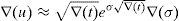
This paper has given practical algorithms allowing us to compute shadow riskless assets and good deals for discrete time arbitrage-free complete pricing models. The interest seems to be clear. Indeed, shadow riskless assets permit managers to reduce the level of capital requirements, whereas good deals permit investors to outperform every alternative strategy if the performance criteria are expected return and risk. Needless to say that return/risk ratios are crucial in order to rank the effectiveness of portfolio managers.
The given algorithms are general since they apply under weak assumptions about the pricing model. Essentially, the existence of good deal is the unique required condition. Nevertheless, for illustrative reasons, numerical experiments have been given for the binomial model. One of the numerical experiments has been built with real American data.
The algorithms allow us to incorporate changes of the model parameters in a dynamic setting. These changes may be caused by both evolutions of the market conditions and/or measurement errors. Nevertheless, it may be also interesting to have a previous information about the possible effect of these changes. The sensitivity of the solutions with respect to important elements has been given. Among other interesting elements, one can consider the pricing rule (or the stochastic discount factor) or the manager's random final pay-off.
This research was partially supported by “WELZIA MANAGEMENT, SGIIC, S.A.”, “Comunidad Autónoma de Madrid” (Spain), Grant S2009/ESP-1594, and “MICIN” (Spain), Grant ECO2009-14457-C04.

