


This article focuses on an integrated production inventory model with rework of the imperfect units and stock dependent demands of the customer from several retailers. There is an opportunity to build a model to measure the amount of carbon emissions during the time of production and the corresponding rate of carbon emission parameters are random which follows Beta distribution. Here, the rate of imperfectness is assumed to be a function of time and production rate. In this paper, a manufacturer–retailer–customer chain system is developed in which the retailer gets an upstream trade credit period from the manufacturer and retailers offer a downstream trade credit period to customers to stimulate demand as well as sales and reduce inventory. The model has been developed as a profit maximization problem with respect to the manufacturer and retailers. Finally, several numerical examples and sensitivity analysis are provided to illustrate the model.
In the past few decades, the classical economic production quantity (EPQ) model assumes that the production system is failures free and that all time produced are perfect quality items (Silver & Peterson, 1985). In a real situation, the production process starts in an in-control state and it may become out-of-control by producing defective items. Porteus (1986) was one of the first to consider the situation where the production process may shift from an ‘in-control’ state to an ‘out-of-control’ state with a given probability each time it produces an item and as a consequence it begins to produce a certain percentage of defective items. Khouja and Mehrez (1994) considered a classical economic production lotsize (EPL) model where the elapsed time for the production process shift to imperfect production is assumed to be an exponential distribution. Salameh and Jaber (2000) proposed a modified production inventory model which accounted for imperfect quality items. Goyal and Cárdenas-Barrón (2002) extended the idea of Salameh and Jaber's (2000) model and proposed a practical approach to determine EPQ for items with imperfect quality. Goyal and Cárdenas-Barrón (2002) have reworked the paper of Salameh and Jaber (2000) and presented a practical approach to find out the optimal lotsize. Chiu (2003) has extended Hayek and Salameh's (2001) model by assuming a portion of the defective items are reworked to make them good quality items instead of reworking on all of the defective items and the remaining items are sold at a price. Annadurai and Uthayakumar (2010) developed an EPQ model with random defective rate with beta distribution. The inspection process monitors the production process which in turn reduces the number of imperfect quality products. Sana (2010) developed two inventory models in an imperfect production system and showed that the inferior quality items could be reworked at a cost where overall production inventory costs could be reduced significantly. Sana (2011) extended the idea of imperfect production process in three layer supply chain management system. Panda and Modak (2015) introduced an inventory model for random replenishment interval and imperfect quality items under demand fluctuation. Modak, Panda, and Sana (2015) presented a complete review over optimal just-in-time buffer inventory for preventive maintenance with imperfect quality items. Recently, researchers have studied the imperfect production inventory problems with different policies. Manna, Das, Dey, and Mondal (2016) investigated a production-inventory model for an imperfect production system with repairable items and promotional demand. Later, Manna, Dey, and Mondal (2017) introduced a lot-sizing problem for a defective manufacturing system with advertisement dependent demand and manufacturing rate dependent of defective rate.
In today's highly competitive business world, the Supply Chain Management (SCM) is a vital issue for manufacturers, retailers, and customers. It is an improvement methodology to improve the business performance. As a result, SCM are in the form to enhance the revenue and reduced operational costs, improved flow of supplies, reduction in delays of production and increased customer satisfaction. Researchers as well as practitioners in manufacturing industries have given importance to develop inventory control problems in supply chain management. In his pioneer work, Khouja (2003) addressed optimizing inventory decisions in a multistage multi customer supply chain. Modak, Panda, and Sana (2016) developed a three-echelon supply chain coordination considering duopolistic retailers with perfect quality products. Manna, Dey, and Mondal (2014) investigated a three-layer supply chain in an imperfect production inventory model with two storage facilities under fuzzy rough environment. Panda, Modak, and Basu (2014) derived a disposal cost sharing and bargaining for coordination and profit division in a three-echelon supply chain. Later, Panda and Modak (2016) explored the effects of social responsibility on coordination and profit division in a supply chain. Further, Panda, Modak, and Cárdenas-Barrón (2017) dealt with a problem of coordinating a socially responsible closed-loop supply chain with product recycling. Recent reviews on supply chain management are provided by Chaharsooghi, Heydari, and Zegordi (2008), Munson and Rosenblatt (2001), Wang, Wee, and Tsao (2010), and Yao, Evers, and Dresner (2007).
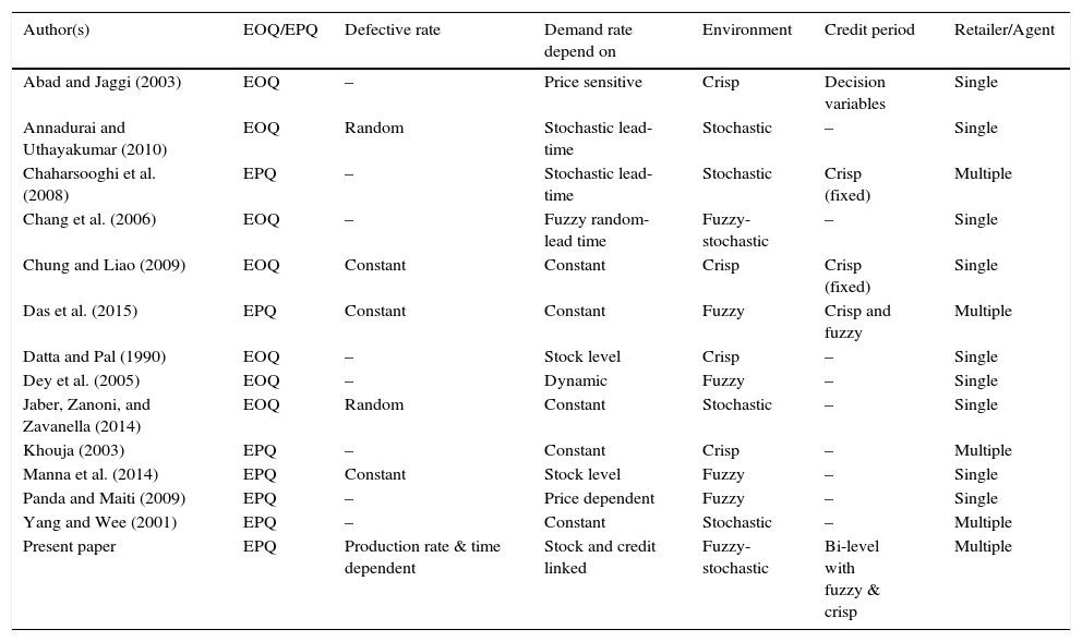
In present business culture, usually suppliers offer a permissible delay in payments to manufacturer, manufacturer offers a permissible delay in payments to retailer, and retailer offers a permissible delay in payments to customers, known as trade credit period, in paying for purchasing cost, which is a very common business practice. Suppliers often offer trade credit as a marketing strategy to increase sales and reduce on hand stock level. Once a trade credit has been offered, the amount of period that the retailer's capital tied up in stock is reduced, and that leads to a reduction in the retailer's holding cost of finance. In addition, during trade credit period, the retailer can accumulate revenues by selling items and by earning interests. As a matter of fact, retailers, especially small businesses which tend to have a limited number of financing opportunities, rely on trade credit as a source of short-term funds. In this research field, Goyal and Cárdenas-Barrón (2002) establish a classical economic order quantity (EOQ) model with a constant demand rate under the condition of permissible delay in payments. Chung and Liao (2009) studied a lot-sizing problem under a supplier's trade credit depending on the retailer's order quantity. Abad and Jaggi (2003) developed a seller–buyer model under permissible delay in payments by game theory to determine the optimal unit price with trade credit period considering that the demand rate is a function of the retail price. Recently, Das, Das, and Mondal (2015) developed an integrated model under trade credit policy. The detailed comparative statement of the proposed model with the existing literature is presented in Table 1.
Summary of related literature for supply chain models.
| Author(s) | EOQ/EPQ | Defective rate | Demand rate depend on | Environment | Credit period | Retailer/Agent |
|---|---|---|---|---|---|---|
| Abad and Jaggi (2003) | EOQ | – | Price sensitive | Crisp | Decision variables | Single |
| Annadurai and Uthayakumar (2010) | EOQ | Random | Stochastic lead-time | Stochastic | – | Single |
| Chaharsooghi et al. (2008) | EPQ | – | Stochastic lead-time | Stochastic | Crisp (fixed) | Multiple |
| Chang et al. (2006) | EOQ | – | Fuzzy random-lead time | Fuzzy-stochastic | – | Single |
| Chung and Liao (2009) | EOQ | Constant | Constant | Crisp | Crisp (fixed) | Single |
| Das et al. (2015) | EPQ | Constant | Constant | Fuzzy | Crisp and fuzzy | Multiple |
| Datta and Pal (1990) | EOQ | – | Stock level | Crisp | – | Single |
| Dey et al. (2005) | EOQ | – | Dynamic | Fuzzy | – | Single |
| Jaber, Zanoni, and Zavanella (2014) | EOQ | Random | Constant | Stochastic | – | Single |
| Khouja (2003) | EPQ | – | Constant | Crisp | – | Multiple |
| Manna et al. (2014) | EPQ | Constant | Stock level | Fuzzy | – | Single |
| Panda and Maiti (2009) | EPQ | – | Price dependent | Fuzzy | – | Single |
| Yang and Wee (2001) | EPQ | – | Constant | Stochastic | – | Multiple |
| Present paper | EPQ | Production rate & time dependent | Stock and credit linked | Fuzzy-stochastic | Bi-level with fuzzy & crisp | Multiple |
The basic well known EOQ model was first introduced by Harris (1915). The model is based on the assumption of constant demand without any deterioration function. However, in reality, the demand may increase or fall in the course of time. According to Levin, Mclaughlin, Lamone, and Kottas (1972), the presence of inventory has a motivational effect on the people around it. Now-a-days, with the advent of multi-nationals in the developing countries, there is a stiff competition amongst the multi-nationals to capture the market. Thus, in the recent competitive market, the inventory/stock is decoratively exhibited and colorably displayed through electronic media to attract the customers and thus to boost the sale. For this reason, Datta and Pal (1990) consider linear form of stock dependent demand.
In recent years, the green house effect and global warming have gained much attention due to strong and more frequent extreme weather events. In developing countries, there is a scope of measuring and maintaining such carbon-emission. Benjaafar, Li, and Daskin (2013) first presented a series of model formulations that illustrate how carbon emission considerations can be incorporated in to decision-making problem. Dye and Yang (2015) study a deteriorating inventory system under various carbon emissions policies.
Uncertainty of the parameters in decision making is a well established phenomenon in recent years. Estimation of such parameters in the objective functions using traditional econometric methods is not always possible due to the insufficient historical data, especially for newly launched products. Generally, nature of uncertainties can be classified into three major groups – random (stochastic), fuzzy (imprecise), and rough (approximation). Several research works on fuzzy inventory problem (Chang, Yao, & Ouyang, 2006; Dey, Kar, & Maiti, 2005) have been presented in the literature. Panda and Maiti (2009) extended the single period inventory problem in a multi-product manufacturing system under chance and imprecise constraints. Chang (2004) has developed an EOQ model with fuzzy defective rate and demand. More recently, Das et al. (2015) and Manna et al. (2014) considered different imprecise parameters in their supply chain models.
This paper considers a manufacturer–retailer–customer supply chain model involving bi-level trade credit and random carbon emission. In this paper, a two-echelon supply chain system with several markets is considered. By taking the imperfect production process into consideration, we establish a bi-level trade credit model to enhance the demand of the customers, which actually is a Stackelberg model with the customer's satisfaction and whole system being the leader in the management. Here, we introduce an integrated production-inventory model with rework policy. The manufacturer offers trade credit period to retailer and retailer offers trade credit to the customers. Both the credit periods are fuzzy in nature and defuzzified using the expression of expectation. The demand of the customers is considered stock dependent.
The remainder of this paper is organized as follows. In Section 2, we present the notations and assumptions employed throughout this paper. Section 3 develops an economic production inventory model for the optimization of production time and expected profit. Section 4 contains basic concepts on fuzzy sets and develops different cases of the proposed model for manufacturer credit period (M˜), retailers’ credit period (N1, N2). Section 5 presents a solution methodology and algorithm to obtain optimal solutions of fuzzy stochastic problem. Several numerical examples and managerial insights of the illustrate model are presented in Section 6. Then, we perform a sensitivity analysis in Section 7. Finally, Section 8 contains a summary of the paper and some concluding remarks with future research directions.
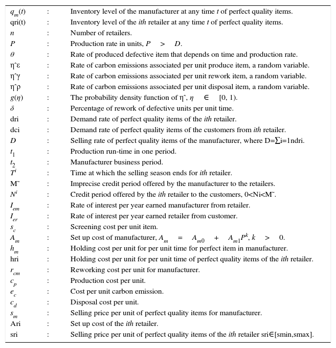
2Notations and assumptionsTo develop the model, the following notations and assumptions have been used.
2.1Notations| qm(t) | : | Inventory level of the manufacturer at any time t of perfect quality items. |
| qri(t) | : | Inventory level of the ith retailer at any time t of perfect quality items. |
| n | : | Number of retailers. |
| P | : | Production rate in units, P>D. |
| θ | : | Rate of produced defective item that depends on time and production rate. |
| ηˆε | : | Rate of carbon emissions associated per unit produce item, a random variable. |
| ηˆγ | : | Rate of carbon emissions associated per unit rework item, a random variable. |
| ηˆρ | : | Rate of carbon emissions associated per unit disposal item, a random variable. |
| g(η) | : | The probability density function of ηˆ, η∈[0, 1). |
| δ | : | Percentage of rework of defective units per unit time. |
| dri | : | Demand rate of perfect quality items of the ith retailer. |
| dci | : | Demand rate of perfect quality items of the customers from ith retailer. |
| D | : | Selling rate of perfect quality items of the manufacturer, where D=∑i=1ndri. |
| t1 | : | Production run-time in one period. |
| t2 | : | Manufacturer business period. |
| Ti | : | Time at which the selling season ends for ith retailer. |
| M˜ | : | Imprecise credit period offered by the manufacturer to the retailers. |
| Ni | : | Credit period offered by the ith retailer to the customers, 0 |
| Iem | : | Rate of interest per year earned manufacturer from retailer. |
| Ier | : | Rate of interest per year earned retailer from customer. |
| sc | : | Screening cost per unit item. |
| Am | : | Set up cost of manufacturer, Am=Am0+Am1Pk, k>0. |
| hm | : | Holding cost per unit for per unit time for perfect item in manufacturer. |
| hri | : | Holding cost per unit for per unit time of perfect quality items of the ith retailer. |
| rcm | : | Reworking cost per unit for manufacturer. |
| cp | : | Production cost per unit. |
| ec | : | Cost per unit carbon emission. |
| cd | : | Disposal cost per unit. |
| sm | : | Selling price per unit of perfect quality items for manufacturer. |
| Ari | : | Set up cost of the ith retailer. |
| sri | : | Selling price per unit of perfect quality items of the ith retailer sri∈[smin,smax]. |
- 1)
Manufacturer produces a mixture of perfect and imperfect quality items. Some portion of imperfect items are reworked and transformed into perfect quality items.
- 2)
The defective rate is not constant, it increased with time and production rate. So, the defective rate depends on time and production rate. It is defined as follows: θ=β+λP+ξt, where β, λ and ξ are positive constants as well as taken suitable values.
- 3)
The demand rate of the customers depend on displayed stock/inventory of the item and the credit period offered, i.e., dci=dc0i+dc1ieμNi+d1iqri(t), dc0i>0,dc1i>0,d1i>0,μ>0
- 4)
The production-project might involve rolling out clean energy technologies or soaking up carbon emission from the production that need to be included in a production problem as a carbon emission cost.
- 5)
Set up cost of manufacturer has been considered as production rate dependent.
- 6)
It is assumed that the fuzzy credit period (M˜) offered by supplier must be within replenishment period (T), i.e., M˜
- 7)
The ith retailer provides a down-stream credit period (Ni) to his/her customers, where Ni
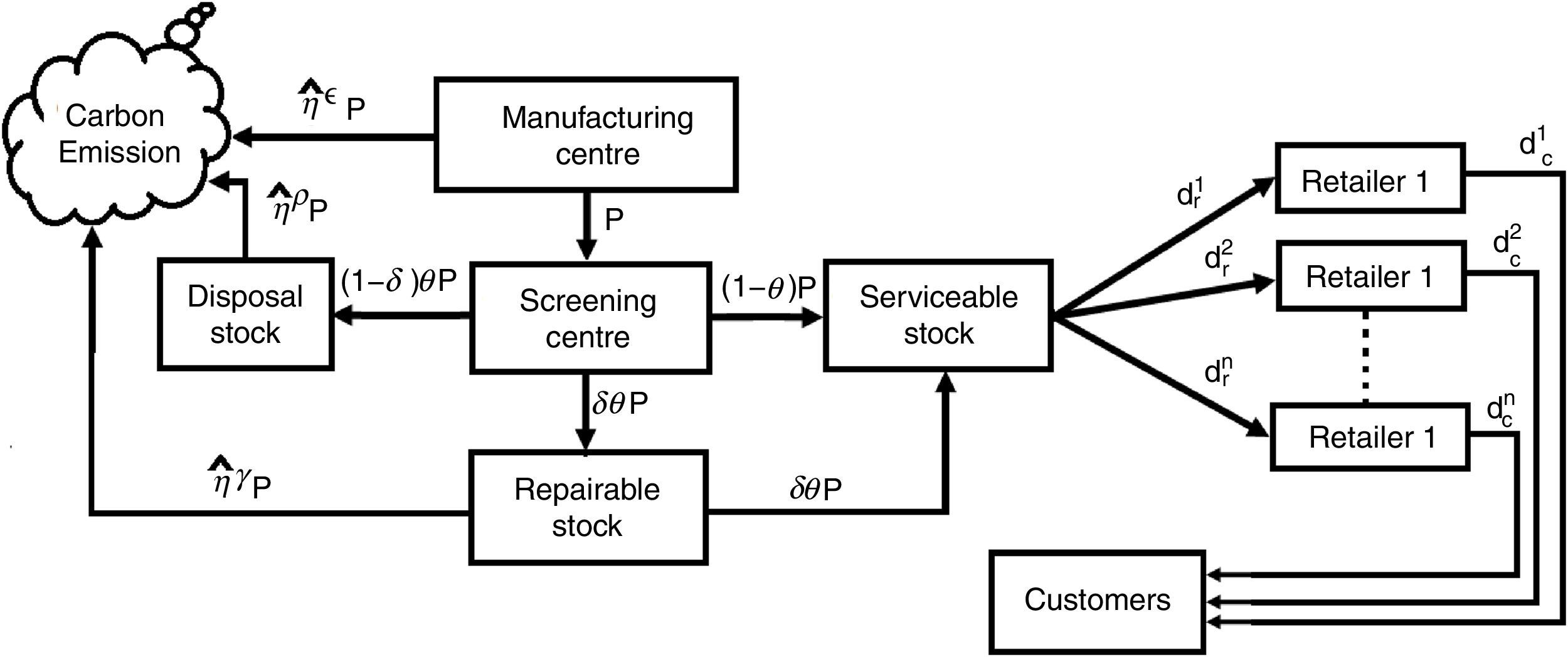
We consider a manufacturing system which produces both perfect and imperfect items in each production run at rates (1−θ)P and θP respectively. Among the imperfect items, few are repaired at a rate δθP portion. We consider a manufacturing system which produces the lot size Q in each production run, with constant production and demand rates denoted by p and d, respectively. In this process of production, screening and repaired unavoidable carbons are emited at rates η¿, ηρ and ηγ respectively. The fresh units are transported to several markets with their individual demand along with an imprecise trade credit M˜. The retailers sold the units in their respective markets as per customers demand dci(t)=dc0i+dc1ieμiNi+d1iqri(t). Here it necessary to mention that the demand depends on the displayed stock of the retailer and the credit period Ni offered to the customers. Such a supply chain inventory model is derived to formulate different cost expression (Fig. 1).
3.1Mathematical formulation of the manufacturer
The rate of change of inventory level of manufacturer for perfect quality items can be represented by the following differential equations:
with boundary conditions qm(0)=0, qm(t2)=0.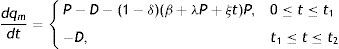
The solution of above differential equations are given by
Lemma 1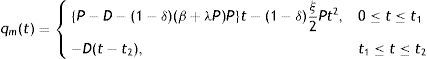
The manufacturer's production time length (t1) and production rate (P) must satisfy the conditiont2=1D{P−(1−δ)(β+λP)P}t1−(1−δ)ξP2Dt12.
Proof: From the continuity conditions of qm(t) at t=t1, the following is obtained,
{P−D−(1−δ)(β+λP)P}t1−(1−δ)ξ2Pt12=−D(t1−t2)⇒Pt1−(1−δ)(β+λP)Pt1−(1−δ)ξ2Pt12=Dt2⇒t2=1D{P−(1−δ)(β+λP)P}t1−(1−δ)ξP2Dt12
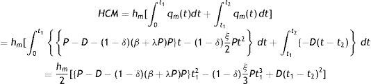
Inventory holding cost for perfect items is
Production cost for the manufacturer = cpPt1.
Inspection cost = scPt1.
Reworking cost for manufacture = rcm∫0t1δ(β+λP+ξt)Pdt=rcmδβ+λP+ξ2t1Pt1
Set up cost of the manufacturer=Am.
Revenue of perfect quality items for the manufacturer = smdrt2.
Disposal cost during (0,t2)=cd(1−δ)β+λP+ξ2t1Pt1
The total amount of carbon emissions during the production run time can be calculated as follows:
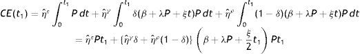
The expected carbon emission cost during the production run time is given by:

Expected total profit Πm(t1) of manufacturer during the period (0, T) is given by:
3.2Formulation of the ith retailer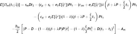
The ith retailer receives his/her required quantity per unit time dri from the manufacturer and fulfils the customers’ demand rate dci. Those retailers start their business on or before the production run time t1, pay r portion of the price amount payable initially and the remaining (1−r) portion is paid at the end of his/her business period. But those retailers arrive after the production run time t1, pay the total amount at their business starting time. They pay the initial amount by getting loans from banks at the rate of interest of Ip per year. Every retailer earns interest at the rate of Ie by depositing sales revenue continuously. The inventory level qri(t) for the ith retailer is governed by the following differential equation:
with boundary conditions qri(0)=0 and qri(Ti)=0.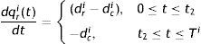
The customer demand is dci(t)=dc0i+dc1ieμiNi+d1iqri(t)=d0i+d1iqri(t), where d0i=dc0i+dc1ieμNi.
Therefore the solutions of above differential equations are given by:
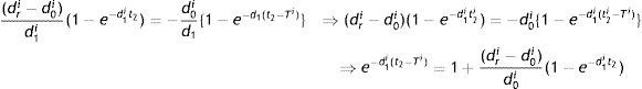
Lemma 2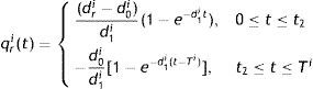
The retailer time length of inventory (Ti) is given by:
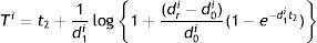
Proof: From the continuity conditions of qri(t) at t=t2, we have
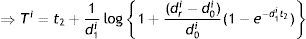
Holding cost of the ith retailer is given by
Holding cost (HCR) for all retailers’ is given by

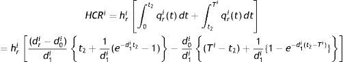
Sales revenue from perfect quality items of the ith retailer is given by
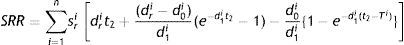
All retailers’ total sales revenue (SRR) is given by:
All retailers’ total purchase cost (PCR) is given by: PCR=∑i=1nsmdrit2
Here it is assumed that the retailer's trade credit period offered by the manufacturer is M and that of customer's offered by the retailer is Ni (where Ni<M). The retailer is charged by the manufacturer an interest rate of Ip per year per unit for the unpaid amount after the delay period and can earn an interest at the rate of Ie (Ie>Ip) per year per unit for the amount sold during the period (Ni,M) respectively. Depending on the cycle times of the retailer and offering as well as receiving credit periods, three different cases may arise, which have been discussed separately.
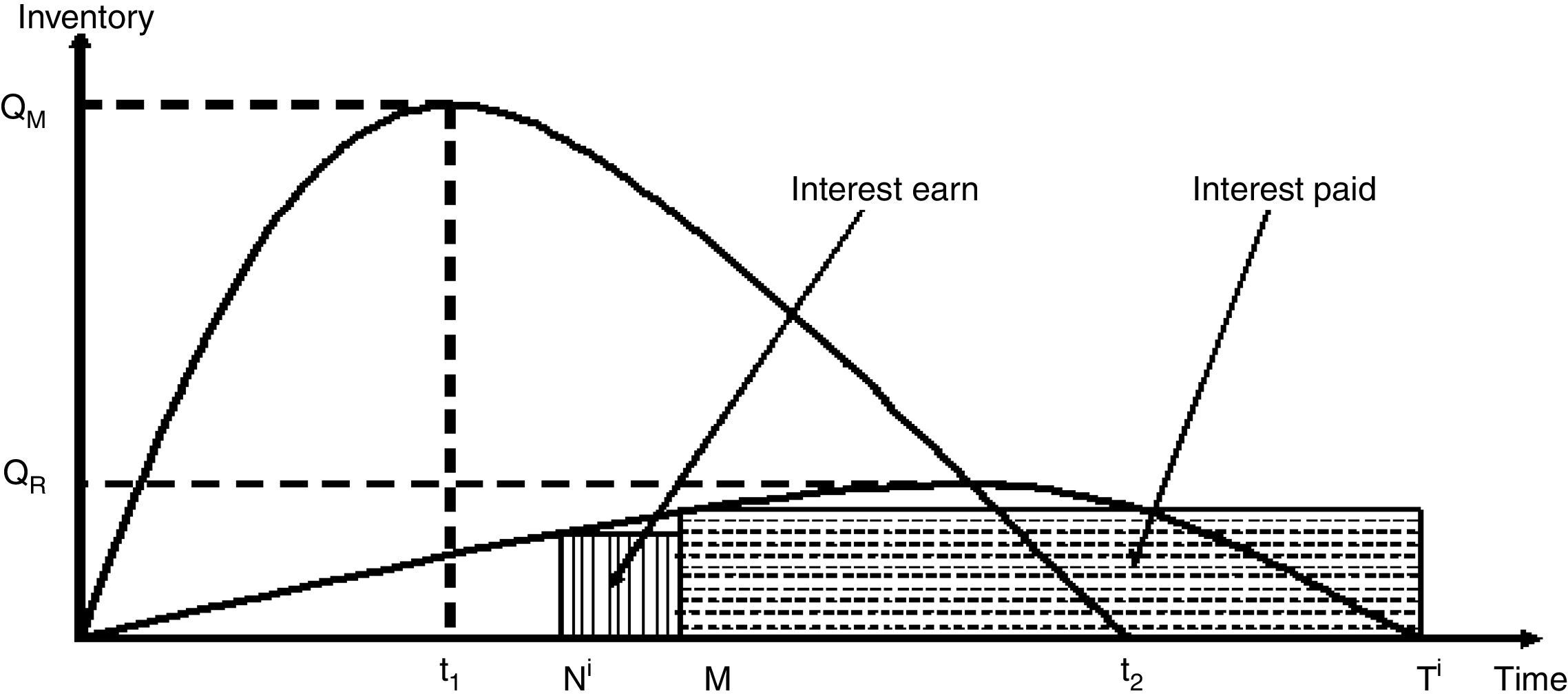
Case 1: Ni<M<t2<Ti
Interest paid by the ith retailer (IP1i) is (Fig. 2):
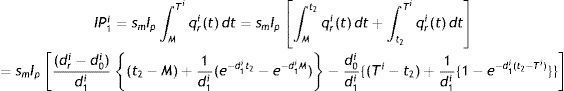

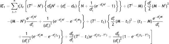
Interest earned by the ith retailer (IE1i) is:
All retailers’ total interest payable (IP1) is expressed as:

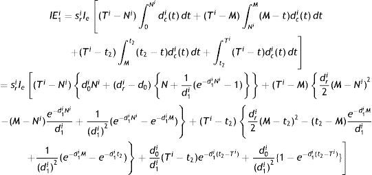
All retailers’ total interest earned (IE1) is obtained as:
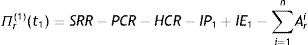
Therefore, all retailers’ total profit is given by:
The total profit (ITP) for this case of the integrated system is written as:
E[ITP1(t1;ηˆ)]=E[Π(t1;ηˆ)]+Πr(1)(t1)
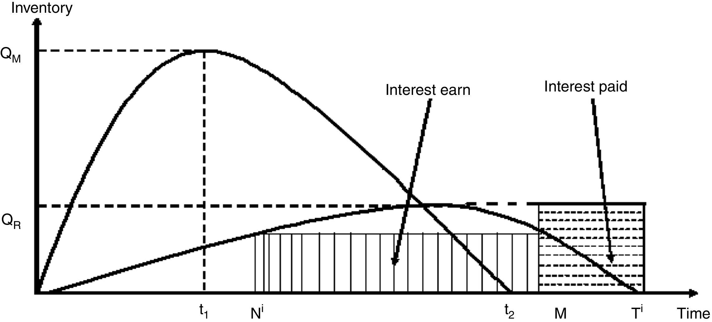
Case 2: Ni<t2<M<Ti (Fig. 3)

Interest paid by the retailer (IP2i) is IP2i=smIp∫MTiqri(t) dt=smIp∫MTi−d0id1i[1−e−d1i(t−Ti)] dt=d0ismIpd1i1d1i{e−d1i(M−Ti)−1}−(Ti−M)
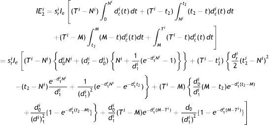
Interest earned by the retailer (IE2i) is:
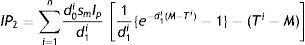
All retailers’ total interest payable (IP2) is expressed as
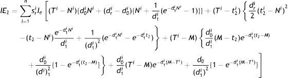
All retailers’ total interest earned (IE2) is obtained as:
Therefore, all retailers’ total profit is given by:
Πr(2)(t1)=SRR−PCR−HCR−IP2+IE2−∑i=1nAri
The total profit (ITP) for this case of the integrated system is written as:
E[ITP2(t1;ηˆ)]=E[Π(t1;ηˆ)]+Πr(2)(t1)
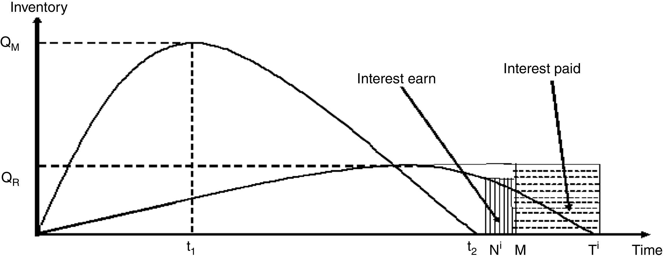
Case 3: t2<Ni<M<Ti
Interest paid by the retailer (IP3i) is (Fig. 4): IP3i=smIp∫MTiqri(t) dt=smIp∫MTi−d0id1i[1−e−d1i(t−Ti)] dt=d0smIpd1i1d1i{e−d1i(M−Ti)−1}−(Ti−M)

Interest earned by the retailer (IE3i) is:
All retailers’ total interest payable (IP3) is expressed as:
IP3=∑i=1nd0smIpd1i1d1i{e−d1i(M−Ti)−1}−(Ti−M)
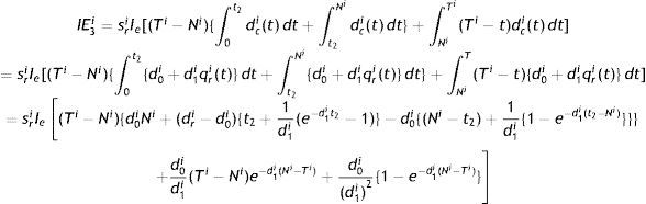
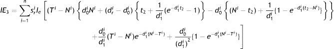
All retailers’ total interest earned (IE3) is obtained as:
Therefore, all retailers’ total profit is given by:
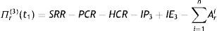
So, the total profit (ITP) for this case of the integrated system is written as:
E[ITP3(t1;ηˆ)]=E[Π(t1;ηˆ)]+Πr(3)(t1)
When manufacturer and retailers’ have decided to share resources to undertake mutually beneficial cooperation, the joint total profit which is a function of t1 can be obtained by maximized E[ITP(t1;ηˆ)] and is given by:
4Basic concepts on fuzzy sets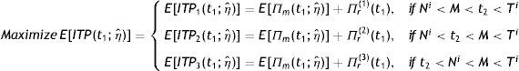
The fuzzy set theory was developed to define and solve the complex system with sources of uncertainty or imprecision which are non-statistical in nature. The fuzzy set theory is a theory of graded concept (a matter of degree) but different from a theory of chance or probability. The term fuzzy was proposed by Zadeh (1965). A short delineation of the fuzzy set theory is given below.
Fuzzy set: A fuzzy set is a class of objects in which there is no sharp boundary between those objects that belong to the class and those that do not. Let X be a collection of objects and x be an element of X, then a fuzzy set à in X is a set of ordered pairs A˜={(x,μA˜(x))/x∈X}
where μA˜(x) is called the membership function or grade of membership of x in A˜ which maps X to the membership space M which is considered as the closed interval [0,1].
Note: When M consists of only two points 0 and 1, Ã becomes a non-fuzzy set (or Crisp set) and μA˜(x) reduces to the characteristic function of the non-fuzzy set (or crisp set).
Fuzzy number: A fuzzy number is a special class of a fuzzy sets. Different definitions and properties of fuzzy numbers are encountered in the literature but they all agree on that a fuzzy number represents the conception of a set of real numbers close to a, where a is the number being fuzzyfied.
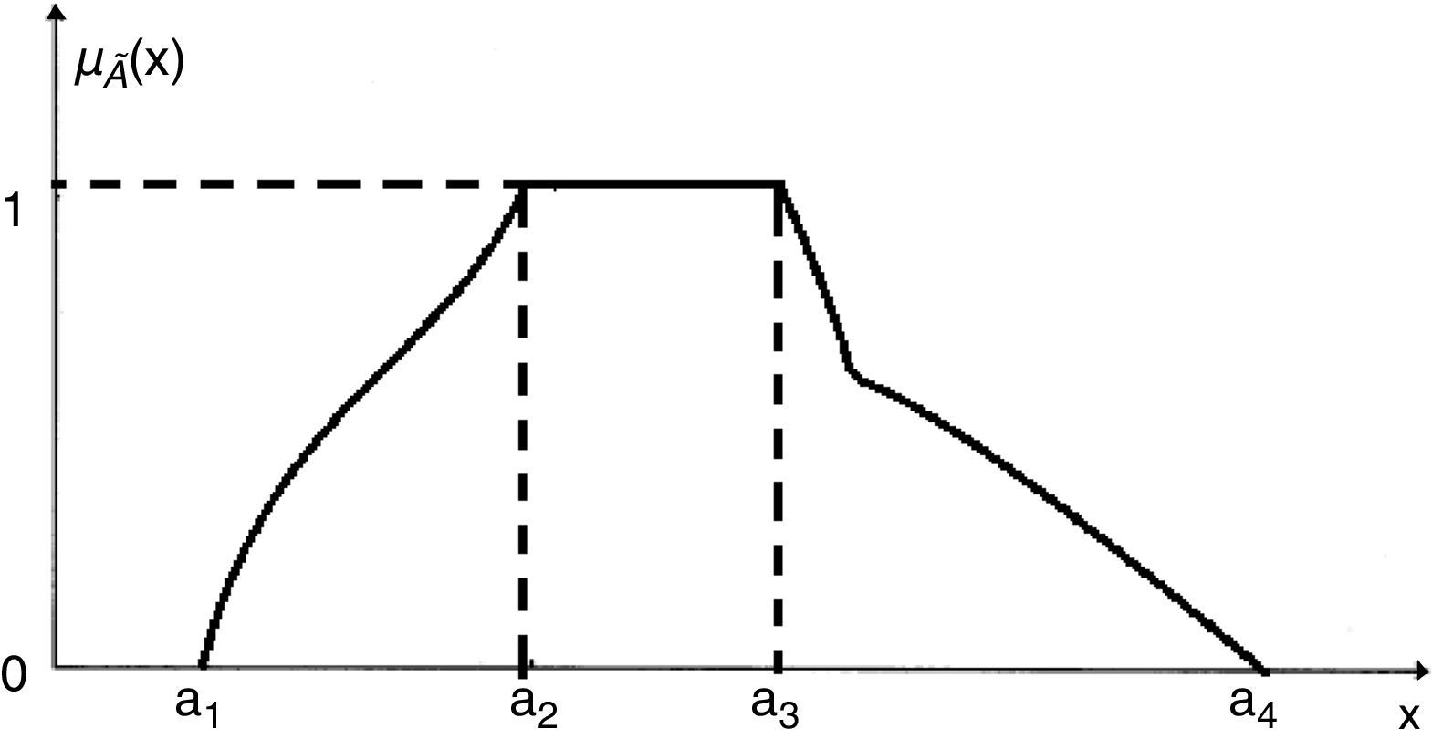
A fuzzy number is a fuzzy set in the universe of discourse ℜ whose membership function μA˜(x) is
- i.
a continuous mapping from ℜ to the closed interval [0,1],
- ii.
constant on −∞,a1:μA˜(x)=0,∀x∈−∞,a1,
- iii.
strictly increasing on [a1, a2]: e.g., μA˜(x)=f(x),∀x∈[a1,a2] where f(x) is a strictly increasing function of x,
- iv.
constant on [a2, a3]: e.g., μA˜(x)=1,∀x∈[a2,a3],
- v.
strictly decreasing on [a3, a4], e.g., μA˜(x)=g(x),∀x∈[a3,a4] where g(x) is a strictly decreasing function of x,
- vi.
constant on a4,∞: e.g., μA˜(x)=0,∀x∈a4,∞.
A general shape of a fuzzy number following the above definition may be shown pictorially as in Fig. 5. Here, a1, a2, a3 and a4 are real numbers. A fuzzy number à in ℜ is said to be discrete or continuous according as its membership function μA˜(x) is discrete or continuous.
.")
Note 1: When the membership function are linear and increasing from a1 to a2, and decreasing from a2 to a3 such fuzzy number is known as triangular fuzzy number (TFN).
Note 2: When the membership function are linear and increasing from a1 to a2, constant between a2 to a3 and decreasing from a3 to a4 such fuzzy number is known as trapezoidal fuzzy number (TrFN).
Zadeh's extension principle: One of the basic concepts of fuzzy set theory which is used to generalize crisp mathematical concepts to fuzzy sets is the extension principle. Let X and Y be two universes and f: X→Y be a crisp function. The extension principle tells us how to induce a mapping f: P(X)→P(Y), where P(X) and P(Y) are the power sets of X and Y respectively.
Following Zadeh (1978) we define the fuzzy extension principle as follows:
We have the mapping f: X→Y, y=f(x) which induce a function f: A˜→B˜ such that B˜ = f(A˜) = {((y,μB˜(y))|y=f(x),x∈X)}, where
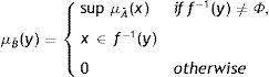
Centroid of the fuzzy number: The centroid value of a fuzzy function ϕM˜ is given by
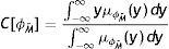
For a triangular fuzzy number (TFN) A˜=(a−Δ1,a,a+Δ2), where 0<Δ1<a and 0<Δ2, Δ1, Δ2 are determined by the decision makers. Then the centroid value, C[A˜]=a+13(Δ1+Δ2)
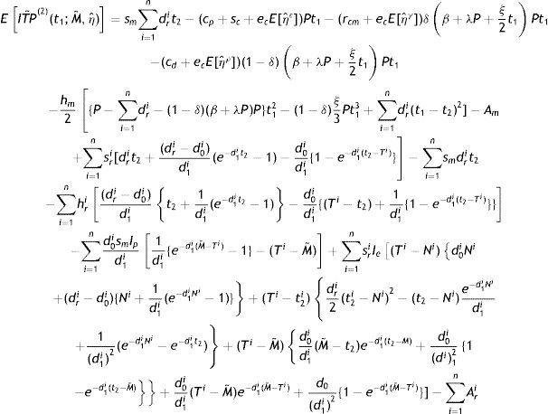
4.1Model with fuzzy credit periodWe assume that the manufacturer gives an opportunity to all the retailers by offering a fuzzy credit period (M˜). Here, the credit period M˜ is represented in form of triangular fuzzy number. So due to fuzzy credit period (M˜), the optimum value of integrated profit function ITP(t1) will be different for various values of M˜ with some degree of belongingness. Therefore, in such a situation, the profit function will be fuzzy in nature and is denoted by ITP˜(t1;M˜,ηˆ), where:
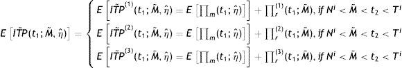
The imprecise expressions of EITP˜(1)(t1;M˜,ηˆ), EITP˜(2)(t1;M˜,ηˆ) and EITP˜(3)(t1;M˜,ηˆ) are given below:
and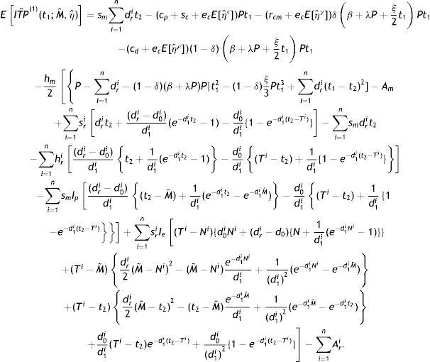
EITP˜(2)(t1;M˜,ηˆ)=sm∑i=1ndrit2−(cp+sc+ecE[ηˆε])Pt1−(rcm+ecE[ηˆγ])δβ+λP+ξ2t1Pt1−(cd+ecE[ηˆρ])(1−δ)β+λP+ξ2t1Pt1−hm2[{P−∑i=1ndri−(1−δ)(β+λP)P}t12−(1−δ)ξ3Pt13+∑i=1ndri(t1−t2)2]−Am+∑i=1nsri[drit2+(dri−d0i)d1i(e−d1it2−1)−d0id1i{1−e−d1i(t2−Ti)}]−∑i=1nsmdrit2−∑i=1nhri(dri−d0i)d1it2+1d1i(e−d1it2−1)−d0id1i(Ti−t2)+1d1i{1−e−d1i(t2−Ti)}−∑i=1nd0smIpd1i1d1i{e−d1i(M˜−Ti)−1}−(Ti−M˜)+∑i=1nsriIe(Ti−Ni)d0iNi+(dri−d0i)t2+1d1i(e−d1it2−1)−d0i{(Ni−t2)+1d1i{1−e−d1i(t2−Ni)}}}+d0id1i(Ti−Ni)e−d1i(Ni−Ti)+d0i(d1i)2{1−e−d1i(Ni−Ti)}−∑i=1nAri.
5Solution methodologyThe proposed non-linear problem of model are solved by a gradient based non-linear optimization method – Generalized Reduced Gradient Method using LINGO Solver 12.0 for particular input data.
5.1Algorithm to get the optimum valuesThe optimum values production time (t1) and expected total profit for the fuzzy stochastic model are obtained through algorithm.
Step 1: For the random variable 'ηˆ' with p.d.f ‘g(η)’ evaluate the expected value of integrated total profit ITP˜(1)(t1;M˜,ηˆ), ITP˜(2)(t1;M˜,ηˆ) and ITP˜(3)(t1;M˜,ηˆ) using the definition EITP˜(1)(t1;M˜,ηˆ)=∫−∞∞ITP˜(1)(t1;M˜,ηˆ)g(η)d(η), similarly obtained EITP˜(2)(t1;M˜,ηˆ) and EITP˜(3)(t1;M˜,ηˆ)
Step 2: For a given triangular fuzzy number (TFN) M˜=(M−Δ1,M,M+Δ2), the fuzzy expressions of EITPM˜(1)=EITP˜(1)=(EITPl(1),EITPm(1),EITPr(1)), EITPM˜(2)=EITP˜(2)=(EITPl(2),EITPm(2),EITPr(2)) and EITPM˜(3)=EITP˜(3)=(EITPl(3),EITPm(3),EITPr(3)) are obtained using fuzzy extension principal.
Step 3: Then from the fuzzy expressions EITP˜(1)(t1;M˜,ηˆ), EITP˜(2)(t1;M˜,ηˆ) and EITP˜(3)(t1;M˜,ηˆ) obtained the centroid values CEITP(1)=CEITPM˜(1), CEITP(2)=CEITPM˜(2) and CEITP(3)=CEITPM˜(3) respectively, using the definition presents in Section 4, which is the process of defuzzification.
Step 4: Finally, maximized each CEITP(1)(t1), CEITP(2)(t1) and CEITP(3)(t1) with respect to the decision variable t1 by using LINGO Solver 12.0 for particular input data.
Example 1 We consider a production-inventory supply chain model with the following characteristics: P=42 units, β1=0.10, λ=0.001, ξ=0.02, Δ1=0.01, Δ2=0.02, δ=0.70, cp=$32 per unit, csr=$2 per unit, rcm=$10 per unit, cd=$5 per unit, hm=$4 per unit per unit time, hr(1)=$4.5 per unit per unit time, hr(2)=$4.8 per unit per unit time, Ar(m0)=$140, Ar(m1)=$130, Ar(1)=$140, Ar(2)=$130, sm=$140 per unit, sr(1)=$260 per unit, sr(2)=$250 per unit, ec=$2.5 per unit, smin=$220, smax=$280, dr(1)=17 unit, dr(2)=18 unit, dc0(1)=9.84 unit, dc0(2)=9.54 unit, dc1(1)=1.8, dc1(2)=3, d1(1)=7, d1(2)=6, μ(1)=7, μ(2)=6.
The respective carbon-emission rates ηˆε, ηˆγ and ηˆρ for production process, rework process and disposal units followed a Beta distribution g(η) with parameters v,w i.e., the p.d.f. of η is:
g(η)=ηv−1(1−η)w−1β(v,w),0≤η≤10,otherwise
For ¿=1, γ=2 and ρ=3, we have:
E[ηˆε]=vv+w,E[ηˆγ]=v(v+1)(v+w)(v+w+1) and θ=β+λP
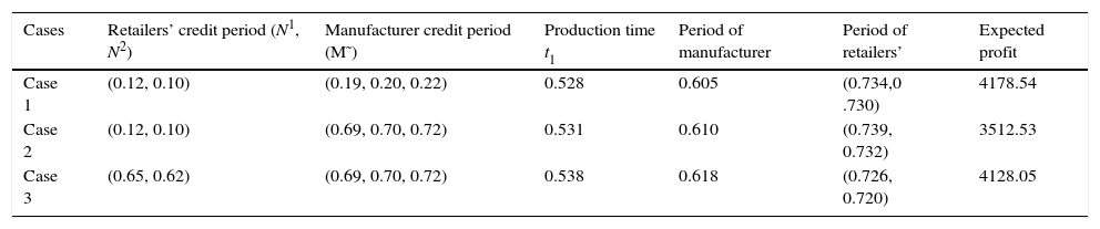
Applying the proposed computational algorithm yields the results shown in Table 2 for different cases.
Optimal results of different cases when θ=β+λP+ξt.
| Cases | Retailers’ credit period (N1, N2) | Manufacturer credit period (M˜) | Production time t1 | Period of manufacturer | Period of retailers’ | Expected profit |
|---|---|---|---|---|---|---|
| Case 1 | (0.12, 0.10) | (0.19, 0.20, 0.22) | 0.528 | 0.605 | (0.734,0 .730) | 4178.54 |
| Case 2 | (0.12, 0.10) | (0.69, 0.70, 0.72) | 0.531 | 0.610 | (0.739, 0.732) | 3512.53 |
| Case 3 | (0.65, 0.62) | (0.69, 0.70, 0.72) | 0.538 | 0.618 | (0.726, 0.720) | 4128.05 |
In manager's point of view, case 2 gives minimum profit. Since in that case manufacturer lost maximum opportunity of credit period, where as the customers receive maximum benefit from the management system. The first and last cases are nearly same in terms of profit since in the first case both the members offer lower credit period and in the last case both the members offer higher credit periods. More over, in the third case, as retailer offers higher credit period, the demand of the customers becomes high but the quantity transferred from manufacturer to retailer is the same, therefore, period of consumptions of the retailer is reduced. As the demand of the customers are linked with the credit period offered by the retailer, high demand of the customers reduced the time period of the retailers.Example 2 Evaluate the optimal policy of the decision maker when the defective rate of produce item depends on production rate only (i.e., ξ=0) and the remain parameters of the system are unalter.
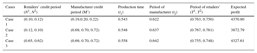
Table 3 shows the optimum policies of the decision maker when the defective rate of the produced item is of the form θ=β+λP.
Optimal results of different cases when θ=β+λP.
| Cases | Retailers’ credit period (N1, N2) | Manufacturer credit period (M˜) | Production time (t1) | Period of manufacturer (t2) | Period of retailers’ (T1, T2) | Expected profit |
|---|---|---|---|---|---|---|
| Case 1 | (0.10, 0.12) | (0.19,0.20, 0.22) | 0.543 | 0.622 | (0.763, 0.750) | 4370.80 |
| Case 2 | (0.12, 0.10) | (0.69, 0.70, 0.72) | 0.548 | 0.637 | (0.767, 0.761) | 3872.79 |
| Case 3 | (0.65, 0.62) | (0.69, 0.70, 0.72) | 0.558 | 0.642 | (0.755, 0.748) | 4327.61 |
In comparison of the cases, Example 2 reveals the same decisions as Example 1. Moreover, when defective rate does not depend on time, the defective units are quite less, i.e., fresh units are more than that of Example 1. So, business periods are larger than the Example 1, which also yield more profit than Example 1 for each cases.Example 3 Find the optimal policies of the decision maker when the defective rate of produce item depend on time only (i.e., λ=0) and the remain parameters of the system are unaltered.
When the defective rate of produce item does not depend on production rate but depends on time only, i.e., θ=β+ξt, then the optimum results are shown in the following Table 4.
Optimal results of different cases when θ=β+ξt.
| Cases | Retailers’ credit period (N1, N2) | Manufacturer credit period (M˜) | Production time (t1) | Period of manufacturer (t2) | Period of retailers’ (T1, T2) | Expected profit |
|---|---|---|---|---|---|---|
| Case 1 | (0.10, 0.12) | (0.19, 0.20, 0.22) | 0.728 | 0.848 | (1.020, 1.010) | 6074.09 |
| Case 2 | (0.12, 0.10) | (0.69, 0.70, 0.72) | 0.731 | 0.851 | (1.023, 1.013) | 6833.38 |
| Case 3 | (0.65, 0.62) | (0.69, 0.70, 0.72) | 0.739 | 0.858 | (0.998, 0.991) | 6095.70 |
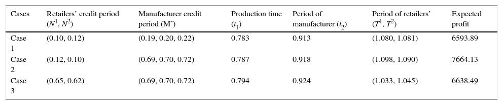
If defective rate does not depend on the production rate, then production time is much larger. So manufacturer produces more quantity of items. For this reason, the periods of manufacturer and retailers are more than the scenarios when θ=β+λP+ξt or θ=β+λP. So the optimum profit is more than the other two scenarios, as expected.Example 4 When the defective rate of produce item is constant (i.e., λ=0 and ξ=0) then evaluate the optimal profit of the decision maker (the remain parameter of the system remain unalter).
From Table 5, it is concluded that when defective rate is fixed then the optimum profits are maximum for each cases. This is due to the less amount of defective units. The other conclusions regarding the comparison of the three cases remain the same as in Example 1.
Optimal results of different cases when θ=β.
| Cases | Retailers’ credit period (N1, N2) | Manufacturer credit period (M˜) | Production time (t1) | Period of manufacturer (t2) | Period of retailers’ (T1, T2) | Expected profit |
|---|---|---|---|---|---|---|
| Case 1 | (0.10, 0.12) | (0.19, 0.20, 0.22) | 0.783 | 0.913 | (1.080, 1.081) | 6593.89 |
| Case 2 | (0.12, 0.10) | (0.69, 0.70, 0.72) | 0.787 | 0.918 | (1.098, 1.090) | 7664.13 |
| Case 3 | (0.65, 0.62) | (0.69, 0.70, 0.72) | 0.794 | 0.924 | (1.033, 1.045) | 6638.49 |
In this section, we examine the effects of changes in the system parameters. A sensitivity analysis is performed by changing some of the parameters as follows. On the basis of the results calculated the following observations can be made.
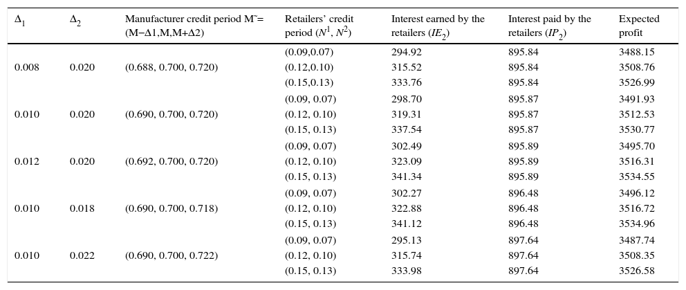
Sensitivity analysis 1: This example outlines the effects of changes in the different values of trade credit period M˜ and N's. The results are given in Table 6.
Sensitivity analysis on different values of trade credit period M˜ and N's case 2.
| Δ1 | Δ2 | Manufacturer credit period M˜=(M−Δ1,M,M+Δ2) | Retailers’ credit period (N1, N2) | Interest earned by the retailers (IE2) | Interest paid by the retailers (IP2) | Expected profit |
|---|---|---|---|---|---|---|
| (0.09,0.07) | 294.92 | 895.84 | 3488.15 | |||
| 0.008 | 0.020 | (0.688, 0.700, 0.720) | (0.12,0.10) | 315.52 | 895.84 | 3508.76 |
| (0.15,0.13) | 333.76 | 895.84 | 3526.99 | |||
| (0.09, 0.07) | 298.70 | 895.87 | 3491.93 | |||
| 0.010 | 0.020 | (0.690, 0.700, 0.720) | (0.12, 0.10) | 319.31 | 895.87 | 3512.53 |
| (0.15, 0.13) | 337.54 | 895.87 | 3530.77 | |||
| (0.09, 0.07) | 302.49 | 895.89 | 3495.70 | |||
| 0.012 | 0.020 | (0.692, 0.700, 0.720) | (0.12, 0.10) | 323.09 | 895.89 | 3516.31 |
| (0.15, 0.13) | 341.34 | 895.89 | 3534.55 | |||
| (0.09, 0.07) | 302.27 | 896.48 | 3496.12 | |||
| 0.010 | 0.018 | (0.690, 0.700, 0.718) | (0.12, 0.10) | 322.88 | 896.48 | 3516.72 |
| (0.15, 0.13) | 341.12 | 896.48 | 3534.96 | |||
| (0.09, 0.07) | 295.13 | 897.64 | 3487.74 | |||
| 0.010 | 0.022 | (0.690, 0.700, 0.722) | (0.12, 0.10) | 315.74 | 897.64 | 3508.35 |
| (0.15, 0.13) | 333.98 | 897.64 | 3526.58 | |||
Table 6 of sensitivity analysis 1 shows that more spread of fuzzy credit period gives lower profit of the system as well as lower interest paid by the retailer (as expected). And increasing of down stream credit period (offered by the retailer to the customers) of the system yields more earn of the retailer due to the increasing of demand which consequently decreases the holding cost also.
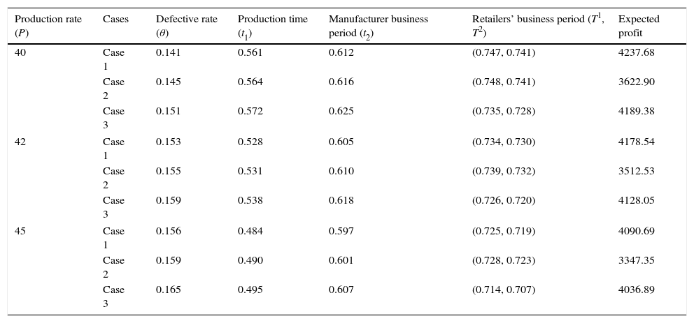
Sensitivity analysis 2: In this example, we use the same data as in Example 1 except the production rate on the optimal solution. The results are presented in Table 7.
Optimal results for all cases when changing the value of production rate (P).
| Production rate (P) | Cases | Defective rate (θ) | Production time (t1) | Manufacturer business period (t2) | Retailers’ business period (T1, T2) | Expected profit |
|---|---|---|---|---|---|---|
| 40 | Case 1 | 0.141 | 0.561 | 0.612 | (0.747, 0.741) | 4237.68 |
| Case 2 | 0.145 | 0.564 | 0.616 | (0.748, 0.741) | 3622.90 | |
| Case 3 | 0.151 | 0.572 | 0.625 | (0.735, 0.728) | 4189.38 | |
| 42 | Case 1 | 0.153 | 0.528 | 0.605 | (0.734, 0.730) | 4178.54 |
| Case 2 | 0.155 | 0.531 | 0.610 | (0.739, 0.732) | 3512.53 | |
| Case 3 | 0.159 | 0.538 | 0.618 | (0.726, 0.720) | 4128.05 | |
| 45 | Case 1 | 0.156 | 0.484 | 0.597 | (0.725, 0.719) | 4090.69 |
| Case 2 | 0.159 | 0.490 | 0.601 | (0.728, 0.723) | 3347.35 | |
| Case 3 | 0.165 | 0.495 | 0.607 | (0.714, 0.707) | 4036.89 | |
Here, we conclude that increasing rate of production (P) increases the rate of defectiveness (θ) as it is a increasing function of P, it also reduced value of production time, manufacturing time as well as expected profit due to the increase of production with fixed demand expand the inventory/holding cost. Again, increasing defective amount reduced the amount of fresh unit that caused lower business period and lower profit.
8Conclusions and future researchThis paper develops an integrated production inventory model involving manufacturer, retailer and customers with up-stream and down stream credit periods. This paper will provide the following decision making:
- •
If manufacturer produces an item with defective quality also, then the rate of defective may depend on production-rate and/or time. And the effect of these dependencies are shown here numerically with efficient cause.
- •
The duration of upstream credit period may fluctuate due to different cause, in this regard here, an imprecise nature of upstream credit period is considered and analyzed numerically and mathematically. Moreover, its effects are justified by a sensitivity analysis.
- •
Here, an unavoidable circumstance of carbon-emission is taken into account for a good gesture of society and this emission rate is not fixed through the cycle time, so it is formulated with random nature.
- •
Furthermore, we discuss some special cases of credit periods to show their effect on the management.
- •
Finally, we run several numerical examples and sensitivity analysis to illustrate the problem and provide some managerial insights.
We suggest several possible directions for future research. First, one may extend our considered EPQ model to joint optimization of expected total profit and carbon emission (i.e., maximize expected total profit and minimize carbon emission). Second, one immediate possible extension could be allowable shortages, cash discounts, etc. Finally, one can extend the fully trade credit policy to the partial trade credit policy in which a seller requests its credit-risk customers to pay a fraction of the purchase amount at the time of placing an order as a collateral deposit, and then grants a permissible delay on the rest of the purchase amount.
