

This paper deals with a single item deteriorating production inventory model with price sensitive demand. Items deteriorate at a constant rate. The rate of production is finite and controlled by modern technology, capital investment and number of labors. Demand is adjusted by flexibility of inventory level and this flexibility is introduced through the determination of optimal production stopping time, number of labors and unit selling price of the product. The total profit is determined by trading of selling price, production cost, deterioration cost and holding cost. The paper aims to maximize total profit per unit time in a production cycle. A real coded genetic algorithm is proposed to find out maximum total profit per unit time and to determine optimal production stopping time, number of labors and unit selling price of the product. Finally, a sensitivity analysis is performed to indicate the effects of the parameters on total profit, unit selling price, number of labors and optimal production stopping time.
After the introduction of Wilson's square root formula (Wilson, 1934) under the assumption of constant demand rate in the earlier part of twentieth century, the EOQ inventory models have long been attracting considerable volume of research attention. For the last twenty five years or so forth, researchers in this area have extended investigation for various models with consideration of item shortage, item order cycles, item deterioration, various demand patterns, item production plans as well as their combinations. In the context of the demand pattern, it is found in real market that the demand of a product is always in dynamic state and this dynamicity occurs due to variability of time, price or even of the instantaneous level of inventory displayed in retail shop. The variability in demand rate was started with the work of Silver and Meal (1969), who determined the EOQ by a heuristic approach in the general case of a deterministic time dependent demand pattern. Donaldson (1977) gave a full analytic solution of the inventory replenishment problem with linear trend in demand over a finite time horizon. Peterson and Silver (1979) noted that sales at the retail level tend to be proportional to inventory displayed. In the last few years, researchers like Baker and Urban (1988), Datta and Pal (1990), Mondal and Phaujdar (1989), and Pal, Goswami, and Chaudhuri (1993) focused on the analysis of inventory system which described the demand rate as a power function and dependent on the level of on hand inventory. However, many super market managers have observed that a portion of the buyers is directly related to the amount of selling price of some products and the sales are affected for higher price of the product. This situation can be expressed mathematically by considering the demand as linear in selling price, a constant demand minus a portion of demand loss due to the price sensitivity (Modak, Panda, & Sana, 2015, Modak, Panda, & Sana, 2016a, 2016b, 2016c; Panda & Modak, 2016). In this research, we have considered the demand as linear price sensitive and this is quite justified for some items like vegetables, fruits, fishes, in which some demands are lost due to the price sensitivity. Nahmias (1982) classified perish ability in terms of fixed life time and random lifetime. Fixed lifetime products (e.g. human blood, drugs) have a deterministic self-life while the random lifetime scenario assumes that the useful life of each unit is a random variable. The random lifetime scenario is closely related to the case of an inventory that experiences continuous physical depletion due to deterioration or decay. Ghare and Schrader (1963) were the first proponents for developing a model with constant decaying rate and they categorized it into three types: direct spoilage, physical depletion and deterioration. Thereafter, a lot of work has been done on deteriorating inventory system. Researches on deteriorating items are important because in real life, milk, drug, food, vegetables do deteriorate significantly. Deterioration is defined by Yang and Wee (2003) as decay, damage, spoilage, evaporation, obsolescence, loss of utility, or loss of marginal value of a commodity that results in decreasing usefulness form the original one. Sarkar, Mandal, and Sarkar (2017) formulated a deteriorating inventory model under stock-dependent consumption rate to determine the optimal replenishment and preservation technology investment strategies. Panda, Modak, and Basu (2014) used disposal cost sharing mechanism for coordination to overcome the product deterioration problem. In this direction, the work of Giri and Chaudhuri (1998), Sana (2008, 2010a, 2010b, 2011a, 2011b, 2012a, 2012b, 2013, 2015), Sana and Chaudhuri (2004), and Sarkar (2013, 2016) should be noted.
All the above researches are restricted to pure inventory replenishment situations i.e. items are purchased or ordered in batches. On the other hand researches on production inventory models have emphasized on various production factors, the setup time, production learning and forgetting effects etc. Peterson and Silver (1979) represented a model where the setup cost and unit variable manufacturing cost are constant and independent of order quantities. Sule (1981) studied the effects of learning and forgetting in the determination of economic product quantity. Again the classical Economic Production Lot Scheduling (EPLS) model (Hax & Candea, 1984) dealt with the availability of inventories at a constant rate where the production rate might be changed (Schweitzer & Seidmann, 1991). Sarkar and Majumder (2013) developed an integrated vendor–buyer supply chain model to reduce the total system cost by considering the setup cost reduction of the vendor. Schweitzer and Seidmann (1991) first introduced the concept of flexibility in the machine production rate and they discussed the processing rate optimization for a flexible manufacturing system (FMS). FMS can be described simply as the manufacturing environment where the production is made according to the demand and the production rate can be slow down or increased according to the decision makers’ desire. Not only that there should be a better coordination among the different sections of the entire production unit. Using preventive maintenance, Modak et al. (2015) proposed a mathematical model to prevent sudden failure as well as maintain the quality of the production system. During the preventive maintenance, a just-in-time buffer inventory is proposed to maintain the normal operation. Silver (1990) enlightened the effects of slowing down the production rate for the production of a family of items assuming a common production cycle for all items and Gallego (1993) extended it to different production cycle for different items. In this direction, the work of Moon, Gallego, and Simchi-Levi (1991), Khouja (1995), Khouja and Mehrez (1994), Kazemi, Olugu, Abdul-Rashid, and Ghazilla (2015), and Panda, Modak, Sana, and Basu (2015) are worth mentioning.
One of the major problems for people dealing with uncertainty-based business is: how to make a better coordination between excessive stocks and shortages. For this, determination of proper selling price of the product is very important due to the price sensitive demand as the sales volume is directly related to it. Again, the hire and fire scenario for the last few years inspired them to determine the exact number of labors for their production. Not only that the intense competition and frequent price reduction of the products by the competitors forced them to make a better coordination between procurement and making decision to get rid of excessive stock due to lower sales volume and shortages when demands are high. This problem further increases when the product deteriorates. The effective way to overcome this problem is to introduce flexibility on inventory level by determining proper production stopping time, proper selling price of the product and proper amount of variable factors of the production system.
In this paper, a manufacturing inventory system is considered where the demand is price sensitive and the items deteriorate at a constant rate. Production process depends on several fixed and variable factors such as buildings, machinery plants, land, raw materials, fuel, power, and ordinary labor. The model considers Cobb–Douglas production function to assess effect of technology, investment and labors on it. This model assumes that applied technology, capital investment and numbers of labors control the rate of production. The objective of the present model is to maximize total profit per unit time in a production cycle. Total profit per unit time, optimal unit selling price of the product and the number of labors are determined by trading of production cost, holding cost and deterioration cost of inventories. A real coded genetic algorithm is used to achieve maximum average profit and to determine optimal production stopping time, number of labors and unit selling price of the product. A numerical example is presented and sensitivity analysis is performed to observe the insight behavior of the model. In this model, our objective is to introduce the flexibility to the volume of inventory by controlling the rate of production through the variation of number of labors and suitably stopping the production unit depending upon the market demand. Thus proper determination of number of ordinary labor and production stopping times that satisfy the maximum profitability is essential.
2Assumptions and notationsThe model is developed under the following assumptions:
- 1.
The rate of production is variable and finite, It is determined by Cobb–Douglas production function which is of the form
where R is the technology which accelerates the rate of production, C is the capital investment except the investment in technology and L is the number of labors. α and (1−α) represent the capital and labor elasticity respectively. - 2.
Demand is price sensitive and is of the form
where a is the scale parameter of the demand rate and b is the demand rate price sensitive parameter. p is the unit selling price of the product. - 3.
A constant fraction θ∈[0, 1], of the storage inventory is deteriorated per unit time.
- 4.
Shortages are not allowed.
- 5.
The lead-time between production and supply is negligible and almost equal to zero.
- 6.
Production rate is greater than demand rate, i.e., P>D.


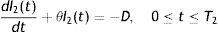
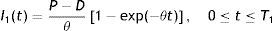
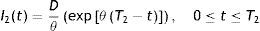
A manufacturing system is considered in which its produced items meet the demand. From the beginning of the production cycle, the items are produced following Cobb–Douglas production rule. It is to be noted that production is a combination of several factors and these factors may be fixed or vary. Buildings, machinery plants, land and top managements are the examples of fixed factors that cannot readily be changed in response to the required changes in the market condition. The variable factor is one whose quantity may be adjusted in response to a change in output or market. Raw materials, fuel, power, ordinary labor etc. are the examples of variable factors. In this model, our objective is to introduce the flexibility of the volume of inventory by controlling the rate of production through the variation of number of labors and suitably stopping the production unit depending upon the market demand. Since demand is sensitive to price, proper determination of selling price is equally important also. Due to the market demand D the inventory level increases at a rate (P−D) units per unit time instead of P units per unit time. The production is continued up to time T1. After time T1, the inventory level decreases gradually at rate D units and ultimately it reaches to zero level at time T2. The instantaneous level of inventory over the cycle time T=T1+T2 is governed by the following differential equations:
with the initial conditions I1(0)=0 and I2(T2)=0. Where I1(t) and I2(t) are the instantaneous level of inventory over the time intervals [0,T1] and [0,T2] respectively.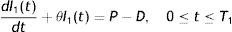
Solving (1) and (2), using the boundary condition, we get
Now, I1(T1)=I2(0) yields
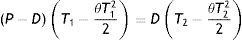
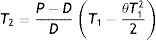
The rate of deterioration is very small, expanding the exponential functions and neglecting second and higher order term of θ we getThus, T2 approximately satisfies the equation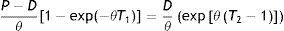
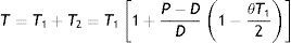
Hence the cycle time T is given by
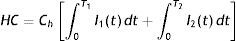
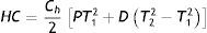
If Ch be the holding cost per unit per unit time, then the holding cost of inventories in the entire production cycle can be found as
After a little bit calculation, we have
However, (PT1−DT) units of inventory are deteriorated in the entire cycle time T. Since p is the selling price of the product, the deterioration cost of the system in the entire production cycle is found as
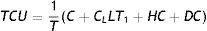
Therefore, total cost per unit time of the system is given bywhere CL is the unit cost of labor.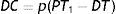
Again, total revenue per unit time can be found as
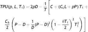
Hence, total profit per unit time in a production cycle is as follows.This, after simplification, yieldswhere T is given by Eq. (7).

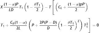
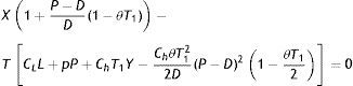
Now, our objective is to maximize TPU(p, L, T1). To evaluate the nature of the profit function in Eq. (12), it is necessary to ascertain whether the function is concave. It is quite impossible to evaluate the Hessian in closed-form to draw the conclusion about its negative definiteness directly. Thus an indirect approach is applied to determine the concavity of TPU(p, L, T1) in Eq. (12). A parametric study is performed over the unit profit function for several values of p, L and T1. The response indicates that TPU(p, L, T1) is concave. Therefore, applying the necessary condition, the values of p, L and T1 which maximizes TPU(p, L, T1) can be obtained by solving simultaneously ∂TPU(p, L, T1)/∂p=0, ∂TPU(p, L, T1)/∂L=0 and ∂TPU(p, L, T1)/∂T1=0. These partial differential equations lead to the following system of non-linear equations.
where Y=P−D+1D(P−D)21−θT122; X=C+(CLL+pP)T1+Ch2Y.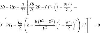
Solution of Eqs. (13)–(15) will give the optimal values of p, L and T1. Substituting these values in (12), optimal value of TPU(p, L, T1) can be found immediately. It is not possible to determine p, L and T1 analytically. Some numerical methods must be used to determine these values. Here, instead of solving simultaneous equations (13)–(15), we have considered TPU(p, L, T1) and used genetic algorithm to determine p, L and T1 as well as unit profit TPU(p, L, T1).
4Numerical exampleIn this section, we consider the suitable variables of the key parameters: a=1000 units, b=20units, CL=$30 per unit per day, CH=$2 per unit per day, C=$40000.00, R=0.9, α=0.6 and θ=0.03. We used here genetic algorithm (GA) (Goldberg, 1989) to find out the maximum value of TPU by determining optimal values of p, L and T1.
A real coded GA is used to maximize TPU. GA is composed of chromosomes and three evolutionary operators: Reproduction, Crossover and Mutation. The initial population is typically generated randomly and then a highly fit population is evolved through several generations by reproducing two individuals using Roulette wheel selection scheme, crossing two individuals using one point crossover with a crossover probability and mutating characters in the resulting individuals with a mutation probability. As GAs have no mathematical convergence proof, till now, a parametric study is carried out by varying the different GA parameters that gives the maximum fitness to the objective function. These parameters include population size, number of generations, crossover probability and mutation probability.
The number of generations is fixed to 50 and the population size is varied, starting from 10 to 100 in step 10. The maximum fitness of the objective function is obtained corresponding to the population size 70. Thus the population size is fixed and number of generations is varied from 10 to 100 in step 10, keeping other parameters fixed to the chosen values and the best result is obtained at 70th generation. In the same manner, we have determined the crossover probability as 0.85 and mutation probability 0.005. For these parametric values of GA, the optimal values are found as p=$26.57, L=10.05≈10, T1=4.15 and consequently TPU=$4876.86, T2=6.96 and T=11.11.
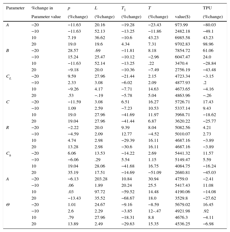
Selection of parameters in the decision-making context is very important. Thus some sensitivity analysis is performed in Table 1 by changing each parameter values by −20%, −10%, 10% and 20% taking one at a time and keeping the remaining unchanged. From Table 1, it is found that the model is low sensitive due to the error in the estimation of the values of CL, R, α, Ch and moderately sensitive due to the error in the estimation of the values of the parameters a, b, C and θ. A simple but realistic phenomenon is found that unit total profit decreases when the rate of deterioration increases. The same is observed for holding cost also. Decreasing value of the price sensitive parameter leads to the increment in total profit. However, there is a close association between demand and capital investment. The common belief that increment in investment increases total profit is found unrealistic.
Percentage change in p, L, T1, T and TPU due to percentage change in parameter values.
| Parameter | %change in | p | L | T1 | T | TPU | |
|---|---|---|---|---|---|---|---|
| Parameter value | (%change) | (%change) | (%change) | (%change) | value($) | (%change) | |
| A | −20 | −11.63 | 20.16 | −19.28 | −23.43 | 973.99 | −80.03 |
| −10 | −11.63 | 52.13 | −13.25 | −11.86 | 2482.18 | −49.1 | |
| 10 | 7.19 | 36.62 | −10.6 | 43.23 | 6985.58 | 43.23 | |
| 20 | 19.0 | 19.6 | 4.34 | 7.31 | 9702.83 | 98.96 | |
| B | −20 | 28.57 | .69 | −11.81 | 8.18 | 7854.72 | 61.06 |
| −10 | 15.24 | 25.47 | −10.12 | −2.96 | 6047.47 | 24.0 | |
| 10 | −11.63 | 52.14 | −13.25 | .22 | 3470.4 | −28.84 | |
| 20 | −9.18 | 20.0 | −10.36 | −7.49 | 2756.19 | −43.48 | |
| CL | −20 | 9.59 | 27.96 | −21.44 | 2.15 | 4723.34 | −3.15 |
| −10 | 2.33 | 3.08 | −6.02 | 2.09 | 4877.93 | .2 | |
| 10 | −9.26 | 4.17 | −7.71 | 14.63 | 4673.65 | −4.16 | |
| 20 | .53 | −.19 | −5.78 | 5.04 | 4863.96 | −.26 | |
| C | −20 | −11.59 | 3.08 | 6.51 | 16.27 | 5726.71 | 17.43 |
| −10 | 1.09 | 2.59 | −7.23 | 10.53 | 5337.14 | 9.43 | |
| 10 | 19.0 | 27.96 | −41.69 | 11.97 | 3968.71 | −18.62 | |
| 20 | 19.04 | 27.96 | −41.44 | 6.87 | 3620.22 | −25.77 | |
| R | −20 | −2.22 | 20.0 | 9.39 | 8.04 | 5082.56 | 4.21 |
| −10 | −4.59 | 2.09 | 12.77 | −4.52 | 5010.07 | 2.73 | |
| 10 | 4.74 | 2.98 | −29.39 | 16.11 | 4687.16 | −3.89 | |
| 20 | 13.28 | 2.98 | −30.6 | 16.11 | 4687.16 | −3.89 | |
| Ch | −20 | 6.06 | 13.53 | −14.22 | 2.69 | 5441.32 | 11.57 |
| −10 | −6.06 | .29 | 5.54 | 1.15 | 5149.47 | 5.59 | |
| 10 | 19.04 | 28.06 | −41.68 | 16.75 | 4084.75 | −16.24 | |
| 20 | 35.19 | 17.51 | −14.69 | −51.09 | 2680.81 | −45.03 | |
| A | −20 | −6.13 | 203.28 | 10.84 | 30.94 | 4759.0 | −2.41 |
| −10 | .06 | 1.89 | 20.24 | 25.5 | 5417.43 | 11.08 | |
| 10 | .03 | 97.72 | −59.52 | 14.48 | 4190.06 | −14.08 | |
| 20 | −13.43 | 35.52 | −68.67 | 18.0 | 3529.8 | −27.62 | |
| Θ | −20 | 1.01 | 24.67 | −9.16 | −8.59 | 5679.02 | 16.45 |
| −10 | 2.6 | 2.29 | −3.85 | 12–.47 | 4921.98 | .92 | |
| 10 | .79 | 27.96 | −18.31 | 8.8 | 4676.3 | −4.11 | |
| 20 | 13.89 | 2.49 | −29.63 | 15.35 | 4536.25 | −6.98 |
Due to −10% and −20% increment in the scale parameter a of demand, TPU increases −49.1% and −80.03% respectively and for the increments −10% and −20% in the capital investment C, TPU increases 9.43% and 17.43% respectively that is lower value of C results higher profit. It indicates that, in a constant demand environment (since the price sensitivity parameter value is very low, b=20 that is 2% of the demand is price sensitive), proper decision for capital investment is essential.
5ConclusionsIn this article, a deteriorating production inventory model with price sensitive demand is developed. The production rate follows Cobb–Douglas rule. The demand is met by the produced inventories whose flexibility is controlled by controlling the production rate, which is determined suitably through the variation of the selling price of the product, number of labors and production stopping time and the flexibility of inventories make a better coordination between excessive stocks and demand. This type of assumption is quite appropriate for people dealing with sea fish, bread, cake etc. and the unorganized sectors of production where the hire and fire scenario is used frequently to control the rate of production. Except some common phenomena (e.g. TPU decreases as the rate of deterioration increases, increment of price sensitivity results in the decrement of TPU and TPU increases as holding cost increases), an interesting relationship between demand and investment is observed. This indicates that investment should be made depending upon the market demand and arbitrary amount of investment may not lead to the maximization of the total profit.
The present model contributes in several directions. Firstly, it considers that the production process depends on the three important factors, applied technology, capital investment and numbers of labors. Secondly, it determines optimal pricing policy under selling price dependent demand. Thirdly, optimal number of labors and optimal production stopping time are determined to maximize the average profit. Fourthly, a parametric study is performed over the unit profit function to check its concavity. Fifthly, maximum fitness of the objective function is tested through a parametric study of different GA parameters (population size, number of generations, crossover probability and mutation probability). Sixthly, a real coded GA is used to determine optimal value of the decision variables. Finally, sensitivity analysis is demonstrated to study the effect of parameters in the decision-making. Application of this model is quite open but proper determination of the parameter values and capital investment in the decision-making context is essential for the successful implementation of this model. The problem under discussion can further be improved for multiple items, imperfect production process and various demand patterns that may also be fuzzy or probabilistic in nature.
