


Considering two samples of Portuguese SMEs: 582 young SMEs and 1654 old SMEs, using the two-step estimation method and quantile regressions, the empirical evidence allows us to conclude that the determinants of investment have a different impact on young and old SMEs, depending on a firm’ level of investment. In the framework of Acceleration Principle and Neoclassical Theories, the determinants are relevant in explaining the investment of young and old SMEs with high levels of investment. The Growth Domestic Product, as the investment determinant of Acceleration Principle Theory, has a greater impact on the investment of young SMEs with high levels of investment. Sales, as the investment determinant of Neoclassical Theory, have greater impact on the investment of old SMEs with high levels of investment. Cash flow, as the investment determinant of Free Cash Flow Theory, is important in explaining the investment of young and old SMEs with low levels of investment. However, cash flow has greater impact on the investment of young SMEs with low levels of investment. The empirical evidence obtained allows us to make suggestions for policy-makers and the owners/managers of Portuguese SMEs.
Various theories have attempted to explain the determinants of firm investment and they can be divided into two major groups: theories, namely Acceleration Principle and Neoclassical Theories that consider the exogenous variables of firm financing decisions as determinants of investment decisions; and theories, namely Free Cash Flow Theory that consider the variables related to firm financing decisions to be fundamental for explaining the firm investment decisions.
When analysing large firms, empirical tests of the explanatory theories of firm investment, considering exogenous variables of firms’ financing decisions as investment determinants, have shown some success. For example, the studies by Chirinko (1993), Aivazian et al. (2005) and Hung and Kuo (2011) indicate that sales are a relevant determinant in explaining firm investment, showing that investment increases when sales increase. However, these results may be influenced by the fact of those studies have analysed large firms.
The smaller size, greater likelihood of bankruptcy, and the ability to change more easily the composition of the assets of SMEs, together with less transparent information provided to creditors (Diamond, 1989) contribute decisively to SME investment being more dependent on internal finance, due to their greater difficulties in accessing external finance. Therefore, we can expect that in SMEs, exogenous variables of firms’ financing decisions, like sales and Gross Domestic Product (GDP), will be less important in explaining investment, with variables related to firm financing decisions becoming more relevant than may be the case in large firms.
Age can serve as a proxy for firm reputation (Diamond, 1989). Older firms’ reputation and past success may allow more advantageous terms in accessing to external finance, with firms becoming less dependent on internal finance to fund their investment opportunities. Indeed, the reputation acquired by firms, through age (Diamond, 1989) may contribute to less relevance of problems of information asymmetry in the relationships between SME owners/managers and creditors. Therefore, for older SMEs, there are other variables, unrelated to financing decisions, such as the economic situation, demand or sales, which are important in their investment decision-making.
Studies about firms’ investment determinants1 do not focus upon the relationships between determinants and investment, neglecting that firms having low or high levels of investment may imply distinct relationships between determinants and investment. Therefore, this study analyses the determinants of firm’ investment and focus on possible differences between firms in different quantiles of investment distribution.
Considering that the age of SMEs may be a determinant of investment opportunities, and the lack of studies investigating the application of the various explanatory theories of investment to firms in general, and to SMEs in particular, the main objective of this paper is to ascertain the applicability of the explanatory theories in young SMEs and old SMEs with different levels of investment.
To fulfil the objective of this study, we consider two samples of Portuguese SMEs2 in the period 2000–2009: 582 young SMEs and 1654 old SMEs, and use the two-step estimation method proposed by Heckman (1979). Initially, probit regressions estimate the inverse Mill's ratio before, turning to quantile regressions to estimate the relationships between determinants and investment in young SMEs and old SMEs.
The current paper contributes for the literature of SMEs’ investment, providing new empirical evidence, because the previous studies have not focused upon small firms with different age and levels of investment. More precisely, the empirical evidence obtained, showing the existence of differences of the impact of the determinants of investment on young and old SMEs with different levels of investment, proves the applicability of the investment theories to young and old SMEs with different levels of investment.
The remainder of the paper is divided as follows. Section ‘Firm investment theories and research hypotheses’ presents the literature review and research hypotheses. Section ‘Methodology’ presents the methodology, namely the database, variables and estimation method used. Section ‘Results and discussion’ presents the results and discussion of the results. Finally, Section ‘Conclusion and implications’ presents the conclusions and implications of the paper.
Firm investment theories and research hypothesesFirm investment theoriesVarious theories explain the factors influencing firm investment. Basically, we can classify them into two major groups: theories considering that investment depends more on conditions outside of the firm, such as sales, demand, growth opportunities and macro-economic conditions; and theories considering that investment depends more on firms’ internal conditions, namely internal finance and liquidity.
Particularly relevant in the first group of theories, explaining firm investment, are those of Keynes (1936) and Kalecki (1937), concerning the influence of demand on investment, Acceleration Principle Theory (Chenery, 1952), Neoclassical Theory (Hall and Jorgenson, 1967; Jorgenson, 1971; Chirinko, 1993), Tobin Q Theory (Tobin, 1969), and the investment theory of Eisner (1978).
According to the theories of Keynes (1936) and Kalecki (1937) firm investment depends on firms’ expectations about future demand. On the one hand, if an increase in the demand is expected, as a consequence of the economic expansion, the firms increase the investment. On the other hand, if a decrease of the demand is expected, as a consequence of a period of economic recession, firms reduce their investment. In accordance with the Acceleration Principle Theory (Chenery, 1952) firms take advantage of favourable conditions allowed by a phase of economic expansion, increasing their investments to maximise their value. In periods of economic recession, when it is less likely that firm profits will increase, firms reduce the investment, adjusting it to the lower business opportunities. According to Neoclassical Theory (Hall and Jorgenson, 1967; Jorgenson, 1971; Chirinko, 1993), firms adjust the investment as a function of their exogenous variables, with sales being especially important in this context. If sales increase, then firms increase investment, but investment diminishes if sales fall. Regarding Tobin Q Theory, if a firms’ market value is higher than the value of their assets, i.e., if the Tobin Q ratio is above 1, firms tend to increase the level of investment, because their market value is higher than the value of their assets as a whole. If firms’ market value is less than the value of their assets, with the Tobin Q ratio being under 1, firms tend to reduce the level of investment, because their market value is less than the total value of their assets, and so a negative adjustment of investment will occur. Finally, according to the investment theory of Eisner (1978), firms adjust the level of investment as a function of variations in sales and profits. On the one hand, firms increase the level of investment, when they predict an increase in sales and profits. On the other hand, firms reduce the level of investment if they forecast a reduction in sales and profits.
In the second group of theories explaining firm investment, the theories of Keynes (1936) and Kalecki (1937), the Liquidity Model (Kuh, 1963), the Managerial Theory of Investment (Baumol, 1967), and the Free Cash Flow Theory (Fazzari et al., 1988; Fazzari and Petersen, 1993) have particular importance due to emphasis on the influence of internal and external finance on investment.
According to the theories of Keynes (1936) and Kalecki (1937), about firm investment, besides the investment in fixed assets being influenced by demand, it depends on firms’ capacity to obtain both internal and external finance. If firms do not have the capacity to generate internal finance, and verify restricted access to external finance, then they decrease the level of investment. According to the Liquidity Model (Kuh, 1963), investment depends on firm liquidity. If firms have the capacity to generate liquidity, they will be able to increase investment. If they face restrictions on liquidity, they will have less investment capacity, and, so they reduce investment. In accordance with the Managerial Theory of Investment (Baumol, 1967), managers prefer to finance the investment through internal funds, due to the greater flexibility in managing this type of finance compared to external finance. According to Free Cash Flow Theory (Fazzari et al., 1988; Fazzari and Petersen, 1993), internal finance, and more specifically cash flow, is important in explaining the firm investment. This importance increases as firms are more restricted in the access to credit, as a consequence of the information asymmetry implicit in the relationships between firm owners/managers and creditors. The fact of firm owners/managers being better informed than creditors about firms’ specific characteristics contributes to creditors to restrain the credit granted. This aspect is particularly important, because, when internal finance is insufficient, the restrictions imposed by creditors may contribute to firms diminishing the investment.
The investment theories described above have been considered in various empirical studies analysing the investment in large firms. The specific characteristics of SMEs that make them different from large firms regarding their environment, structure, decision-making process, flexibility and proximity to markets justify closer scrutiny of some investment theories: Acceleration Principle Theory (Chenery, 1952), because SMEs operate in rather undiversified market niches, therefore their investment is vulnerable to periods of economic recession and expansion; Neoclassical Theory, because SME investment is more vulnerable to exogenous variables, particularly, to sales that allow those firms to evaluate their performance and their level of liquidity (Heshmati and Lööf, 2008); and Free Cash Flow Theory, because the investment of SMEs, particularly the investment of the unquoted SMEs, is heavily dependent on the existence of cash flow (Fazzari et al., 1988), namely when those firms face restrictions in accessing debt.
Research hypothesesIn accordance with Diamond (1989), SME age is a proxy of firm reputation. Therefore, it is expectable that old SMEs obtain debt in more favourable terms, consequently depending less on internal finance, than the younger SMEs. Moreover, according to Fazzari et al. (1988), the existence of firms with low levels of investment suggests that those firms are financially constrained. Young SMEs face more difficulties in obtaining debt, due to their lower age and lower size. It is expectable that the investment determinants in young SMEs with low levels of investment are different from the investment determinants of young SMEs with high levels of investment. Thus, the applicability of firms’ theories to investment decisions of SMEs might be influenced by the age and the level of the investment.
Bernanke and Gertler (1996) state that SMEs, having greater difficulty in diversifying their sources of finance compared to large firms, are more exposed to fluctuations in the economic climate. Therefore, application of Acceleration Principle Theory (Chenery, 1952) to SME investment decisions may be particularly appropriate, since investment in this type of firm may be especially sensitive to fluctuations in the economic situation, increasing in periods of economic growth and diminishing during economic recession.
In periods of economic recession, credit markets impose greater restrictions on borrowing. In addition, in these periods, SMEs are less able to retain cash flow. This being so, in economic recession, SME investment is expected to fall. In periods of economic growth, SMEs may, have, firstly, easier access to credit, and secondly, greater capacity to retain cash flow, these aspects contributing to increase the investment.
The young SMEs with high levels of investment are likely firms with more internal finance, thus less restricted financially, justifying the greater possibility to fund investment opportunities, in the opposite to the situation of young SMES with low levels of investment. We can expect that the marginal effects of economic growth on investment are, particularly, relevant for young SMEs with high levels of investment, given that their greater level of investment suggests that these firms are less financially restricted than young SMEs with low levels of investment.
Based on the discussion presented before, we formulate the following research hypothesis:H1 The importance of the Acceleration Principle Theory, in explaining the investment decisions of young SMEs, depends on the firm level of investment.
The studies by Modigliani and Miller (1958) show that internal and external finance are perfect substitutes. The assumption that the cost of capital is independent on the finance source implies that investment may be funded through any composition of internal finance, debt and external equity.
According to Neoclassical Theory (Hall and Jorgenson, 1967; Jorgenson, 1971; Chirinko, 1993), sales are a factor determinant of firm investment. On the one hand, if sales increase, firms increase investment, but on the other hand, if sales fall they reduce investment. Chirinko (1993), based on sample of large firms, show that sales are statistically predominant over any other explanatory variable of investment. Furthermore, other studies (Aivazian et al., 2005; Hung and Kuo, 2011) identify a positive influence of sales on investment in large firms.
In general, the samples used for, empirical validation of Neoclassical Theory, are essentially made up of large firms (Fazzari et al., 1988). The importance of sales is expected to be lower for SME investment than for large firms’ investment. For small firms, the sales revenues are frequently more relevant in overcoming liquidity difficulties than for funding the investment.
Sales can be expected to be of greater relative importance in explaining the investment of old SMEs than that of young SMEs. Growth of small firms is constrained by internal finance, and in case of financial distress, firms may pass up valuable investment opportunities (Myers and Majluf, 1984). In the beginning of the life-cycle, SMEs are primarily concerned with survival and growth in their operating markets, and less concerned with conquering alternative markets. Moreover, in the first stages of their life-cycle, sales revenues are used mainly to pay down the firms’ start-up expenses rather than channelled to investment. In later stages of the life-cycle, SMEs may adjust investment as a function of sales seeking to diversify their activities and acquire alternative markets. Sales may also be particularly relevant in explaining the investment of SMEs with high levels of investment, since these firms are better prepared to diversify their activities and expand to new markets.
From the above, we formulate the following research hypothesis:H2 The importance of the Neoclassical Theory, in explaining the investment decisions of old SME, depends on the firm level of investment.
Donaldson (1961) conclude that cash flow is an important determinant of firm investment. Furthermore, the importance of cash flow is a consequence of managers’ preferences for finance sources due to the imperfections of the capital markets and uncertainty. The authors state that managers prefer internal finance due to the asymmetry of information with external investors. According to Myers and Majluf (1984), firms prefer internal finance, because the asymmetric information between firms and the capital market increases the cost of external finance. Internal and external finance are not perfect substitutes, given the existence of problems of asymmetric information, making external finance more expensive than internal finance.
Growth of small firms is constrained when internal finance is insufficient, therefore firms may pass up valuable investment opportunities (Myers and Majluf, 1984). Problems of information asymmetry in the relationships between owners/managers of firms and creditors were in the origins of Free Cash Flow Theory (Fazzari et al., 1988; Fazzari and Petersen, 1993). According to this theory, firm investment is not only dependent on exogenous factors, such as sales, but also on endogenous factors, which are particularly important in explaining investment. Fazzari et al. (1988) and Fazzari and Petersen (1993) conclude that cash flow is a relevant determinant in explaining firm investment, and the sensitivity of investment to cash flow variations is greater for firms that face greater financial restrictions. Nevertheless, Kaplan and Zingales (1997, 2000) dispute the conclusions of Fazzari et al. (1988) and Fazzari and Petersen (1993), concluding that the sensitivity of investment to cash flow variations is greater for firms with fewer financial restrictions. On this subject, the conclusions of Moyen (2004) are particularly relevant, showing that conclusions about sensitivity of investment depend on condition of firms to be or not to be financially restricted. Regardless of the greater or lesser sensitivity of investment to cash flow variations, the empirical evidence of various studies3 shows that firms increase the level of investment when they have greater cash flow, but they reduce the level of investment when the cash flow is lower.
Lower age of SMEs implies, firstly, greater business risk, and a consequently greater likelihood of bankruptcy, and secondly, less reputation in credit markets (Diamond, 1989). These characteristics may decisively contribute to lenders making terms of credit difficult for young SMEs, given the greater business risk associated with their activities (Stiglitz and Weiss, 1981; La Rocca et al., 2011).
SME greater likelihood of bankruptcy, less ability to provide collateral, less transparent information available, and greater possibility to change the firm asset composition contribute to lenders to hinder SME access to credit (Diamond, 1989).
The greater likelihood of bankruptcy, less reputation and credibility of young SMEs compared to old ones may decisively contribute to lenders setting less favourable credit terms to young SMEs. In addition, SMEs with low levels of investment probably face greater obstacles in accessing external finance, namely in obtaining debt. Therefore, we can expect that problems of information asymmetry, in the relationships between SME owners/managers and creditors, to be especially important in explaining the investment decisions of young SMEs with low levels of investment.
Therefore, the Free Cash Flow Theory is expected to be particularly applicable to investment decisions of the young SMEs with low levels of investment, given that these firms will bear greater costs in accessing external finance, consequently they are extremely dependent on internal finance to fund their investments.
Based on the arguments presented before, we formulate the following research hypothesis:H3 The importance of Free Cash Flow Theory, in explaining the investment decisions of the young SME, depends on the firm level of investment.
This study uses the SABI (System Analysis of Iberian Balance-Sheets) database, from Bureau van Dijks, for the period 2000–2009.
SMEs are the subject of analysis in this paper. In Portugal, SMEs account for about 99.68% of the total number of firms,4 contributing decisively towards employment and economic growth (National Institute of Statistics, 2010). The study of investment determinants of Portuguese SMEs is particularly important for survival and growth of SMEs, and consequently to increase the employment and economic growth in Portugal.
We select firms based on the European Union recommendation L124/36 (2003/361/CE). According to this recommendation, a firm is considered an SME when it meets two of the following three criteria: fewer than 250 employees; annual total assets under 43 million euros; and business turnover under 50 million euros.
Seeking to solve the problem of possible result bias due to the survival issue, and to obtain a sample more representative of the Portuguese SME situation, we consider two types of SMEs: surviving SMEs in the period of analysis (2000–2009); and non-surviving SMEs in the period of analysis (2000–2009).
Considering that this paper has the purpose to analyse the investment determinants of young and old SMEs with low and high levels of investment, we divide the total sample of Portuguese SMEs into young and old SMEs. Just as Oliveira and Fortunato (2006) and La Rocca et al. (2011), we consider as young SMEs those up to 10 years of age, considering those over 10 years of age as old SMEs.
Based on the criteria mentioned above, we select5: 582 young SMEs, of which 504 survive and 78 do not; and 1654 old SMEs, of which 1326 survive and 328 do not.
Table 1 presents the structure of the database used in this study.
Sample structure of Portuguese SMEs.
| Total SMEs | Young SMEs | Old SMEs | ||||
| SMEs | Observations | SMEs | Observations | SMEs | Observations | |
| Survival SMEs in all period 2000–2009 | 1830 | 15,317 | 504 | 3383 | 1326 | 11,934 |
| Non-survival SMEs exiting in the period 2000–2009 | 406 | 2091 | 78 | 388 | 328 | 1703 |
| Total number of SMEs | 2236 | 582 | 1654 | |||
| Total number of observations | 17,408 | 3771 | 13,637 | |||
Regarding the industry sector structure, we consider the classification used by IAPMEI6 (2008) considering the following industry sectors: Agriculture, Forestry and Mining; Construction; Manufacturing; Trade; Services; and Tourism.
Table 2 presents the industry sector structure of Portuguese firms, as well as the industry sector structure of young and old Portuguese SMEs.
Sectorial structure of Portuguese SMEs.
| Sector | Percentage of total Portuguese SMEs in 2005 | Percentage of total sample of young SMEs in 2000–2009 | Percentage of total sample of old SMEs in 2000–2009 |
| Agriculture, Forestry and Mining | 0.30 | 0.20 | 0.5 |
| Construction | 13.9 | 12.8 | 15.6 |
| Manufacturing | 14.3 | 13.6 | 22.1 |
| Commerce | 31.8 | 29.1 | 27.4 |
| Services | 30.2 | 34.2 | 26.6 |
| Tourism | 9.50 | 10.1 | 7.8 |
We find that firms in trade and services sectors are predominant in Portugal, and this is also the case in terms of these sectors’ representation among young and old SMEs.
Definition of variablesIn accordance with anterior studies (Aivazian et al., 2005; Carbó-Valverde et al., 2008; Martinez-Carrascal and Ferrando, 2008) the dependent variable used in this study is Investment (Ii,t), measured by the ratio between the variation of fixed capital less amortisation and depreciation in the current period and fixed assets in the previous period.
For testing the applicability of the Acceleration Principle Theory to the investment decisions of young and old SME, we consider, as Carbó-Valverde et al. (2008), the explanatory variable of Gross Domestic Product (GDPt) measured by the logarithm of Gross Domestic Product. For testing the applicability of the Neoclassical Theory to the investment decisions of young and old SMEs, we consider the explanatory variable sales (SALESi,t) measured by the logarithm of sales, following the measure used by Martinez-Carrascal and Ferrando (2008). Finally, for testing the applicability of the Free Cash Flow Theory to the investment decisions of young and old SME, we consider the explanatory variable cash flow (CFi,t) measured by the ratio of earnings after tax plus depreciations to total assets, following Aivazian et al. (2005), Carbó-Valverde et al. (2008) and Brown et al. (2009).
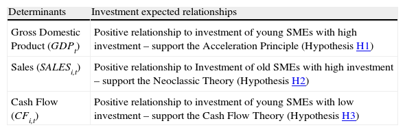
Table 3 presents the relationships between the variables used in the empirical tests of the research hypotheses presented above in Section ‘Research hypotheses’ referring to the validation of the different theories of investment selected.
Determinants and investment expected relationships.
| Determinants | Investment expected relationships |
| Gross Domestic Product (GDPt) | Positive relationship to investment of young SMEs with high investment – support the Acceleration Principle (Hypothesis H1) |
| Sales (SALESi,t) | Positive relationship to Investment of old SMEs with high investment – support the Neoclassic Theory (Hypothesis H2) |
| Cash Flow (CFi,t) | Positive relationship to investment of young SMEs with low investment – support the Cash Flow Theory (Hypothesis H3) |
Martinez-Carrascal and Ferrando (2008) conclude that the level of debt and the costs of debt may be important for the explanation of firms’ investment, mainly in context of SMEs. Additionally, and on the basis of the conclusions of those authors, we consider the debt level and interest rate as variables of control, explaining the investment decisions of young and old SMEs. Following Aivazian et al. (2005) and Martinez-Carrascal and Ferrando (2008), debt level (LEVi,t) is given by the ratio between total liabilities and total assets. In accordance with Martinez-Carrascal and Ferrando (2008), we consider Interest Pay (IPi,t) as interest rate given by the ratio between total interests and total debt.
All the monetary variables were deflated. The base year, taken for deflation of monetary variables, is 2009. It should be noted that all estimations include annual dummy variables, so as to measure other effects of the economic climate, besides those measured by Gross Domestic Product, on variations of investment in young SMEs and old SMEs. In addition, we consider industry sector dummy variables to measure the impact of possible different relationships between determinants and investment, according to young and old SMEs belonging to different industry sectors. We consider sector dummy variables representing the activities presented above: Agriculture, Forestry and Mining; Construction; Manufacturing; Trade; Services; and Tourism.
Estimation methodSurvival analysisEstimating the relationships between determinants and investment, and considering only surviving firms may imply bias of the estimated results as a consequence of not considering the situation of non-surviving firms. In accordance with Calvo (2006) and Lotti et al. (2009), to address the problem of possible result bias, as a consequence of the survival issue, we use the two-step estimation method proposed by Heckman (1979), considering surviving and non-surviving firms.
In a first stage, considering the total sample of young and old SMEs, we estimate probit regressions for firms remaining in the market and for those leaving it. The dependent variable takes the value of 1 if firms survive and the value of 0 if they do not. Just as Calvo (2006), we will consider the determinants used in the second stage of estimation, when we estimate the investment determinants, as explanatory variables of the probit regression.
The probit regression to estimate can be presented as follows:
where GDPt−1 is GDP in the previous period; SALESi,t−1 are sales in the previous period; CFi,t−1 is cash flow in the previous period; LEVi,t−1 is debt in the previous period; IPi,t−1 is the interest paid in the previous period; Ds are industry sector dummy variables; dt are annual dummy variables; and zi,t is the error.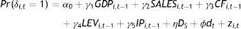
Based on the probit regressions estimated in the first step, we calculate the inverse Mill's ratio,7 and use it, as an additional explanatory variable of investment, in the second step, when estimating relationships between determinants and investment in young SMEs and old SMEs using quantile regressions.
Quantile regressionsModels subject to a quantile regression have received considerable attention, as they allow a more complete statistical analysis of the stochastic relationship between random variables (Koenker and Xiao, 2004; Serrasqueiro et al., 2010).
Given that the purpose of this paper is to ascertain the applicability of the theories explaining investment in young and old SMEs with low and high levels of investment, the most suitable estimation method is quantile regressions.
The values of the dependent variable (i.e., investment) are in ascending order for the different quantiles. Low values of investment are included in low quantiles (5th, 10th, 25th) and high values of investment are included in high quantiles (75th, 90th, 95th).8 Through quantile regressions we can determine if the same independent variables used in a model influence differently the dependent variable in the different quantiles. For example, a given independent variable X can have a negative and statistically significant relationship with the dependent variable Y, when that dependent variable Y has low values, i.e., in the lower quantiles of variable Y distribution (i.e., 5th qt, 10th qt, 25th qt). However, the relationship between variable X and variable Y may be of a different nature when dependent variable Y has high values, i.e., in the upper quantiles of investment distribution (i.e., 75th qt, 90th qt, 95th qt) with, for example, the relationship between X and Y being positive and statistically significant in these circumstances. The major advantage of using quantile regressions is determining whether the relationship between a dependent variable and a set of independent variables depends on the level of the dependent variable. In other words, use of quantile regressions allows us to check whether the relationship between a dependent variable and a set of independent variables is identical for low (i.e., low quantiles) and high (i.e., upper quantiles) levels of the dependent variable.
This study will use the quantile regressions developed by Koenker and Hallock (2001), which can be presented as follows:
in which,where Ii,t is the investment of firm i in the period t; θ are investment distribution quantiles (θ=5th, 10th, 25th, 50th, 75th, 90th, 95th), βθK are the parameters to estimate, in each investment distribution quantile, measuring the relationships between investment determinants and investment; ZK,i,t is the vector representing investment determinants, where ZK,i,t=(GDPt−1; SALESi,t−1; CFi,t−1; LEVi,t−1; IRi,t−1; λi,t; DS; dt), i represents the firm i=[1, …, 504], t is the period t=[1, …, 9] for young SMEs, and i=[1, …, 1326], t is the period t=[1, …, 9] for old SMEs; zθi,t is the error; and Quantθ(Ii,t/ZK,i,t) is the quantile of the dependent variable Ii,t, being conditional in relation to the vector ZK,i,t that refers to the independent variables.

In this way, we seek to study the investment determinants of young SMEs and old SMEs, following a regression subject to quantiles, in which θ=5th, 10th, 25th, 50th, 75th, 90th, 95th. Estimating the quantiles subject to the regression for the different values of θ, we will have the distribution of the variable Ii,t, subject to the corresponding values of ZK,i,t for the values of i(i=1, …, 504) and t(t=1, …, 9) for young SMEs and for the values of i(i=1, …, 1326) and t(t=1, …, 9) for old SMEs. Since our principal objective is to determine the applicability of the theories explaining investment in young SMEs and old SMEs, for different levels of investment, we will consider as quantiles, referring to low investment, the 5th qt, 10th qt and 25th qt, considering as quantiles, referring to high investment, the 75th qt, 90th qt and 95th qt. As the 50th qt is the median of investment distribution, it is not considered as a quantile referring to low or high investment.
Seeking to guarantee the robustness of the results of estimated parameters for the different quantiles, we use the bootstrap matrix method proposed by Buchinsky (1995, 1998). Based on Monte Carlo simulations, Buchinsky (1995) concludes that the bootstrap matrix method is more advisable for data samples with a quite low number of observations, being considered a valid method, in the presence of several types of heterogeneity.
To test for possible non-linearities, in all the investment distribution, for each of the determinants considered in this study, we use the Chow test. For each determinant of investment, the null hypothesis indicates the non-existence of non-linearities between determinants and investment over the investment distribution of young SMEs and old SMEs, the alternative hypothesis indicating the existence of non-linearities between determinants and investment over that distribution.
Results and discussionDescriptive statistics and correlation matricesTable 4 presents the descriptive statistics of the variables used in this study.
Descriptive statistics.
| Variable | Observations | Mean | St. desv. |
| GDPt | 9 | 11.9576 | 0.22756 |
| Variables | Young SMEs | Old SMEs | ||||||
| Firms | Observations | Mean | St. desv. | Firms | Observations | Mean | St. desv. | |
| Ii,t | 582 | 3771 | 0.05561 | 0.19342 | 1654 | 13,637 | 0.04390 | 0.15568 |
| SALESi,t | 582 | 3771 | 14.6912 | 0.28092 | 1654 | 13,637 | 15.4544 | 0.29121 |
| CFi,t | 582 | 3771 | 0.061482 | 0.15766 | 1654 | 13,637 | 0.06675 | 0.17034 |
| LEVi,t | 582 | 3771 | 0.70914 | 0.20431 | 1654 | 13,637 | 0.64908 | 0.19844 |
| IPi,t | 582 | 3771 | 0.05542 | 0.06673 | 1654 | 13,637 | 0.04628 | 0.05819 |
On the basis of the analysis of the descriptive statistics, we conclude that young SMEs have a high level of debt, suggesting that the internal finance may be insufficient to fund their growth opportunities.
Tables 5 and 6 present the correlation matrices regarding the variables used in this study for young SMEs and old SMEs, respectively.
Gujarati and Porter (2010) conclude that the problems of collinearity between explanatory variables are, particularly, relevant when the correlation coefficients between those variables are over 50%. From observation of the correlation coefficients between the explanatory variables, regardless of considering young or old SMEs as the subject of analysis, we conclude that, in no circumstances, there are correlation coefficients over 50%. This being so, problems of collinearity between explanatory variables will not be particularly relevant in this study, regardless of considering young or old SMEs as the subject of analysis.
Investment determinantsIn the appendix, namely in Table A.1, we present the results regarding the survival analysis for young and old SMEs, which refer to the first stage of the estimation method in two stages proposed by Heckman (1979).
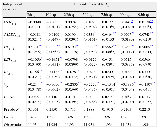
Tables 7 and 8 present the quantile regressions referring to the relationships between determinants and investment for young SMEs and old SMEs, respectively.
Investment determinants – young SMEs.
| Independent variables | Dependent variable: Ii,t | ||||||
| 5th qt | 10th qt | 25th qt | 50th qt | 75th qt | 90th qt | 95th qt | |
| GDPt−1 | 0.0071 (0.0290) | 0.0056 (0.0270) | 0.0104 (0.0305) | 0.0110 (0.0345) | 0.0207** (0.0067) | 0.0245** (0.0076) | 0.0298** (0.0101) |
| SALESi,t−1 | −0.0491** (0.0140) | −0.0349** (0.0115) | −0.0269* (0.0131) | 0.0146 (0.0283) | 0.0290** (0.0089) | 0.0389** (0.0125) | 0.0461** (0.0129) |
| CFi,t.1 | 1.5671** (0.2281) | 1.4516** (0.1754) | 1.3291** (0.1671) | 1.0991** (0.1566) | 0.5717** (0.1291) | 0.3414* (0.1383) | 0.2314* (0.1144) |
| LEVi,t−1 | −0.2177** (0.0560) | −0.2451** (0.0678) | −0.2090** (0.0589) | −0.0807* (0.0389) | 0.1089** (0.0202) | 0.1290** (0.0345) | 0.1508** (0.0389) |
| IPi,t−1 | −0.2898** (0.0577) | −0.2155** (0.0456) | −0.1089** (0.0345) | −0.0451* (0.0240) | 0.0133 (0.0290) | 0.0149 (0.0346) | 0.0103 (0.0307) |
| λi,t | −0.2567** (0.0509) | −0.2891** (0.0678) | −0.2453** (0.0490) | −0.2782** (0.0467) | −0.1901** (0.0445) | −0.2290** (0.0533) | −0.2521** (0.0604) |
| CONS | 0.0145 (0.0308) | 0.0190 (0.0376) | 0.0140 (0.0323) | 0.0244 (0.0379) | 0.0199 (0.0315) | 0.0106 (0.0166) | 0.0118 (0.0187) |
| Pseudo R2 | 0.2934 | 0.2890 | 0.2687 | 0.1822 | 0.3218 | 0.3303 | 0.3115 |
| Firms | 504 | 504 | 504 | 504 | 504 | 504 | 504 |
| Observations | 3383 | 3383 | 3383 | 3383 | 3383 | 3383 | 3383 |
Notes: (1) Standard deviations in parenthesis; (2) the estimates include sectoral dummy variables, but not show; and (3) the estimates include time dummy variables but not show.
Investment determinants – old SMEs.
| Independent variables | Dependent variable: Ii,t | ||||||
| 5th qt | 10th qt | 25th qt | 50th qt | 75th qt | 90th qt | 95th qt | |
| GDPt−1 | −0.0098 0.0344) | −0.0033 (0.0121) | 0.0074 (0.0254) | 0.0102 (0.0502) | 0.0122 (0.0165) | 0.0143* (0.0070) | 0.0178** (0.0064) |
| SALESi,t−1 | −0.0181 (0.0214) | −0.0109 (0.0247) | 0.0190 (0.0391) | 0.0334* (0.0161) | 0.0464** (0.0153) | 0.0607** (0.0189) | 0.0743** (0.0219) |
| CFi,t−1 | 0.5891** (0.1245) | 0.6511** (0.1563) | 0.6190** (0.1178) | 0.5388** (0.0954) | 0.5562** (0.0867) | 0.6223** (0.1112) | 0.5005** (0.0844) |
| LEVi,t−1 | −0.1056* (0.0490) | −0.1451** (0.0331) | −0.0798 (0.0899) | −0.0129 (0.0677) | 0.0451 (0.0891) | 0.0515 (0.0835) | 0.0566 (0.0790) |
| IPi,t−1 | −0.1561** (0.0341) | −0.1133** (0.0259) | −0.0781* (0.0372) | −0.0299 (0.0521) | 0.0209 (0.0575) | 0.0138 (0.0407) | 0.0339 (0.0680) |
| λi,t | −0.2144** (0.0478) | −0.3090** (0.0562) | −0.2805** (0.0569) | −0.2229** (0.0436) | −0.1514** (0.0501) | −0.1886** (0.0494) | −0.1307** (0.0411) |
| CONS | 0.0086 (0.0214) | 0.0140 (0.0225) | 0.0171 (0.0394) | 0.0202 (0.0266) | 0.0214 (0.0371) | 0.0167 (0.0209) | 0.0133 (0.0272) |
| Pseudo R2 | 0.1961 | 0.2350 | 0.1715 | 0.1888 | 0.1910 | 0.2103 | 0.2210 |
| Firms | 1326 | 1326 | 1326 | 1326 | 1326 | 1326 | 1326 |
| Observations | 11,934 | 11,934 | 11,934 | 11,934 | 11,934 | 11,934 | 11,934 |
Notes: (1) Standard deviations in parenthesis; (2) the estimates include sectoral dummy variables, but not show; and (3) the estimates include time dummy variables but not show.
The results indicate that: Gross Domestic Product, sales and debt are determinants stimulating investment in young SMEs with high levels of investment; sales, debt and interest paid are restrictive determinants of investment for young SMEs with low levels of investment; and, cash flow is a determinant stimulating investment of young SMEs, regardless of firms’ level of investment. However, the positive impact of cash flow in investment is greater for young SMEs with low levels of investment than for SMEs with high levels of investment.
The results indicate that Gross Domestic Product and sales are determinants stimulating the investment in old SME with high levels of investment; debt and interest paid are restrictive determinants of investment in old SMEs with low levels of investment; and cash flow is a determinant stimulating the investment in old SME, whatever firms’ level of investment.
Regardless of considering young or old SMEs as our subject of analysis, and whatever the level of investment, the relationship between the inverse Mill's ratio and the firm’ investment is negative and statistically significant. These results show that use of the two-step method by Heckman (1979) was effective in solving possible result bias as a consequence of the survival issue.
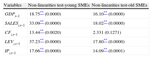
Table 9 presents the results of the tests of possible non-linearities in the relationships between determinants and investment in both young and old SMEs.
Investment determinants of young and old SMEs – F Chow Test to non-linearities.
| Variables | Non-linearities test-young SMEs | Non-linearities test-old SMEs |
| GDPt−1 | 18.75** (0.0000) | 16.10** (0.0000) |
| SALESi,t−1 | 33.09** (0.0000) | 18.02** (0.0000) |
| CFi,t−1 | 13.44** (0.0020) | 2.331 (0.1271) |
| LEVi,t−1 | 37.23** (0.0000) | 17.80** (0.0000) |
| IPi,t−1 | 17.66** (0.0000) | 14.09** (0.0001) |
Note: Probabilities in parenthesis.
Except for the relationship between cash flow and investment in old SMEs, whether taking young SMEs or old SMEs as the subject of analysis, we reject the null hypothesis of equality of estimated coefficients, measuring the relationships between determinants and investment, throughout the investment distribution. We can conclude that, apart from the relationship between cash flow and investment in old SMEs, significant non-linearities are identified in the relationships between determinants and investment, i.e., the kind of the relationship between determinants and investment depends on the level of firm’ investment.
Gross Domestic Product is a positive determinant of investment in young SMEs with high levels of investment, but not for young SMEs with low levels of investment. On the basis of these results we accept the previously formulated Hypothesis H1 as valid, since the GDP, as the determinant used in the framework of Acceleration Principle Theory (Chenery, 1952), is important to explain investment decisions of young SMEs with high levels of investment, but not the investment decisions of young SMEs with low levels of investment.9 The results suggest that young SMEs with high levels of investment are, particularly, concentrated in growth, seeking to reach a minimum scale of efficiency that allows them to survive in their operating markets.
Given that the GDP is a positive determinant of young SMEs with high levels of investment, the results suggest that young SMEs with high levels of investment are able to benefit more efficiently from the evolving economic climate, than young SMEs with low levels of investment. The fact that GDP is not a positive determinant of investment in young SMEs with low levels of investment seems to indicate that these SMEs, probably due to the difficulty in managing their financial resources, are not able to take advantage of favourable development of the economic situation by increasing investment.
The conclusions of Bernanke and Gertler (1996) that SMEs may be more sensitive to the evolving economic climate than large firms, because of the greater difficulty in diversifying their sources of finance, do not appear to be particularly relevant in explaining the empirical evidence identified in this study, since the economic situation does not influence the investment of young SMEs with low levels of investment.
Sales are a positive determinant of investment in old SMEs with high levels of investment, but they are not a positive and not a restrictive determinant of investment in old SMEs with low levels of investment.10 Consequently, the empirical evidence obtained in this study allows us to corroborate the previously formulated Hypothesis H2.
Previous empirical evidence (Aivazian et al., 2005; Hung and Kuo, 2011) indicates that large firms adjust investment as a function of sales. In the current study, young and old SMEs with high levels of investment adjust the investment as a function of sales, but the magnitude of that adjustment is greater for old SMEs with high levels of investment. The empirical evidence obtained, regarding the sales as determinant of investment, allows us to conclude that the principles of the Neoclassical Theory (Hall and Jorgenson, 1967; Jorgenson, 1971; Chirinko, 1993) are verified by SMEs with high levels of investment, mainly by old SMEs with high levels of investment.
We verify that cash flow is a determinant stimulating investment in young SMEs with low and high levels of investment. However, the magnitude of the estimated parameters, measuring the relationships between cash flow and investment, is greater in young SMEs with low levels of investment than in young SMEs with high levels of investment.11 Based on these results, we can consider the previously formulated Hypothesis H3 as valid, since although Free Cash Flow Theory (Fazzari et al., 1988; Fazzari and Petersen, 1993) seem to contribute for understanding young SMEs’ investment decisions, whatever their level of investment. Moreover, Free Cash Flow Theory seems to be more important in explaining the investment decisions of young SMEs with low levels of investment.
As Diamond (1989) concludes, the lower age of SMEs can imply greater business risk, and consequently greater likelihood of bankruptcy, as well as less reputation in credit markets. According to Stiglitz and Weiss (1981) and La Rocca et al. (2011), these characteristics may contribute to lenders setting difficult terms of credit for this type of firms. These arguments seem to be relevant, in explaining the greater importance of cash flow for investment, in young SMEs with low levels of investment. Indeed, SMEs in the start of their life-cycle, with low levels of investment, will presumably be the firms more restricted financially. Considering Donaldson (1961) and Myers and Majluf (1984), the greater relative importance of cash flow, for financing investment in this type of firms, suggests that problems of information asymmetry in the relationships between owners/managers and creditors imply that internal and external finance are not perfect substitutes. Therefore, internal finance is particularly important in the activities of firms, where these problems of information asymmetry are especially relevant.
The empirical evidence obtained in this study corroborates the results of other studies,12 since cash flow is important in explaining SME investment, with investment being adjusted as a function of cash flow.
Regarding the control variables, debt and interest paid are restrictive determinants of investment in young and old SMEs with low levels of investment. However, the magnitude of the estimated parameters, measuring the relationships between debt and investment, and the relationships between interest paid and investment, are greater in young SMEs with low levels of investment than in old SMEs with low levels of investment.13 These results suggest that problems of information asymmetry, in relationships between owners/managers and creditors, are particularly relevant in explaining investment in young SMEs with low levels of investment.
This empirical evidence appears to indicate that certain characteristics of SMEs, such as the greater likelihood of bankruptcy, less capacity to provide collateral, less transparency of available information, and greater possibility to change the composition of firm assets (Diamond, 1989), could be especially relevant for lenders hindering credit and setting credit terms to young SMEs with low levels of investment. In fact, the low levels of investment in young SMEs may be a consequence of the obstacles in accessing credit, implying for these firms to pass up investment opportunities.
It is interesting to confirm that debt is a positive determinant of investment in young SMEs with high levels of investment. This empirical evidence prevents us from corroborating the conclusions of Myers and Majluf (1984) that firms prefer to use internal rather than external finance to fund investment, when our subject of analysis is young SMEs with high levels of investment. Indeed, on the one hand, debt contributes to increase the investment in young SMEs with high levels of investment, the magnitude of the estimated parameter becoming greater as we consider higher quantiles. On the other hand, the magnitude of the estimated parameter measuring the relationship between cash flow and investment becomes lower as we consider higher quantiles.14 These results indicate that the higher the level of investment in young SMEs, the greater the preference for external rather than internal finance to increase investment.
Conclusion and implicationsBased on two samples of Portuguese SMEs: 582 young SMEs and 1654 old SMEs, using the two-step estimation method and quantile regressions, this paper analyses the applicability of theories of investment in young and old SMEs with different levels of investment.
The paper contributes to the literature revealing that age and especially the level of investment are important in explaining investment decisions of SMEs. The Growth Domestic Product, as the investment determinant of Acceleration Principle Theory, has a greater impact in the investment of young SMEs with high levels of investment. The sales, as the investment determinant of Neoclassical Theory, have greater impact in the investment of old SMEs with high levels of investment. Finally, the cash flow, as the investment determinant of Free Cash Flow Theory, has a greater impact in the investment of young SMEs with low levels of investment. The empirical evidence obtained, showing the existence of differences in the impact of the determinants of investment on young and old SMEs with different levels of investment, evidences the applicability of the investment theories to young and old SMEs with different levels of investment.
The results obtained show that the level of debt and the interest rate are restrictive determinants of investment in young SMEs with low levels of investment. These results reinforce the possible dependence of those SMEs on internal finance, as a consequence of their obstacles in obtaining external finance for funding their investment opportunities.
It should be highlighted that in young SMEs with high levels of investment, debt is a positive determinant of investment, becoming relatively more important as investment grows, unlike the case of cash flow whose relative impact diminishes in young SMEs with high levels of investment as the levels of investment become greater. These results are particularly important, showing that when young SMEs carry out major investments they do not necessarily prefer internal to external finance.
Portugal is a country with a bank-based financial system, in which, similarly to some other EU countries, the majority of SMEs do not have access to the stock market. This fact restrains, considerably, the possibility of diversification of SMEs’ financing sources. When internal finance is insufficient Portuguese SMEs are largely dependent on access to debt, on reasonably favourable terms to fund their investment opportunities.
The empirical evidence, obtained in this study, shows that young and old SMEs with low levels of investment may be affected by restrictions in access to debt, this effect being particularly strong in young SMEs with low levels of investment. SMEs in Portugal, as in other European countries, are an important creator of employment, and stimulant of economic growth. Therefore, we suggest policy-makers to support both young and old Portuguese SMEs with low levels of investment, but with good investment opportunities. Above all, the governmental support should be provided through special beneficial lines of credit to young SMEs with low levels of investment, facing credit restrictions, but with good investment opportunities. Therefore, when internal finance is insufficient, those firms do not restrain their investment, nor their growth, increasing their possibility to survive in their operating markets. We suggest that the owners/managers of young and old Portuguese SMEs with low levels of investment try to adjust as far as possible their investment as a function of the economic climate and sales, so as to take advantage of more favourable conditions for increasing investment.
This study contains one limitation. From the database it is not possible to identify variables that would allow us to determine the degree of relationship between the owners/managers of Portuguese SMEs and creditors. Therefore, it is not possible to determine more accurately the consequences of information asymmetry in these relationships. In future studies, seeking to use another database that allows analysing the degree and the kind of relationships between the owners/managers of Portuguese SMEs and creditors, we suggest to analyse the influence of these relationships on the investment decisions of Portuguese SMEs.
Survival analysis – young and old SMEs.
| Independent variables | Dependent variable Pr(δi,t=1) | |
| Young SMEs | Old SMEs | |
| GDPt−1 | 0.0250** (0.0065) | 0.0134** (0.0041) |
| SALESi,t−1 | 0.0561** (0.0124) | 0.0115 (0.0106) |
| CFi,t−1 | 0.4877** (0.1433) | 0.1054 (0.1290) |
| LEVi,t−1 | 0.1890** (0.0562) | 0.1144** (0.0308) |
| IPi,t−1 | −0.1668** (0.0454) | −0.0690* (0.0335) |
| CONS | 0.0111 (0.0456) | 0.0239 (0.0307) |
| Pseudo R2 | 0.4343 | 0.3249 |
| Firms | 582 | 1654 |
| Observations | 3771 | 13,637 |
Notes: (1) Standard deviations in parenthesis; (2) the estimates include sectoral dummy variables, but not show; and (3) the estimates include time dummy variables but not show.
Fazzari et al. (1988), Fazzari and Petersen (1993), Aivazian et al. (2005), Junlu et al. (2009), Sun and Yamori (2009) and Hung and Kuo (2011).
We select Portuguese SMEs according to the European Union recommendation L124/36 (2003/361/CE), i.e., to be considered SMEs, firms must satisfy two of the following criteria: fewer than 250 employees; annual total assets under 43 million euros; and business turnover under 50 million euros.
Fazzari et al. (1988), Fazzari and Petersen (1993), Aivazian et al. (2005), Junlu et al. (2009), Sun and Yamori (2009) and Hung and Kuo (2011).
According to the report of the National Institute of Statistics (2010, p. 1) “in 2008, there were 349,756 micro, small and medium-sized enterprises (SMEs) in Portugal, representing 99.68% of the firms in the non-financial business sector. Micro enterprises were predominant, corresponding to 86% of all SMEs. Employment in non-financial firms was mainly assured by SMEs (72.5%), and SMEs were also responsible for 57.9% of turnover and 59.8% of gross added value at factor cost generated in 2008”. The National Institute of Statistics uses the recommendation of the European Union L124/36 (2003/361/CE) to define an SME. According to the same report (only available in Portuguese language) there are only 1115 large firms in Portugal, which represent 0.32% of the total number of firms in Portugal. We must state that the research sample of this study is composed by SMEs, because they are firms with unique characteristics that make them different from large firms: the majority of Portuguese SMEs are unquoted SMEs and strongly dependent on bank debt.
The Portuguese stock market is rather undeveloped, with access to it being denied to almost all Portuguese SMEs. The research sample is composed by only unquoted Portuguese SMEs. Therefore, in this study it is not possible for us to calculate the Tobin Q as a measure of the growth opportunities of Portuguese SMEs, unlike the studies about the investment determinants of quoted firms, for example, Esteve and Tamarit (1994), Aivazian et al. (2005) and Hung and Kuo (2011).
IAPMEI is a Portuguese governmental institution that provides support to Portuguese SMEs.
To see in detail the formula for calculating the inverse Mill's ratio, consult Heckman (1979).
For example, if a young SME, in a certain period, has a very low level of investment, then the dependent variable, referring to investment, and the correspondent independent variables (GDP, Sales, Cash Flow, Debt, Interest Paid) for that observation will be included in the most inferior quantile of investment, i.e., in the quantis referring to a low levels of investment, for example in the 5th quantile. Considering an old SME, in a given period, with a level of investment very high, then the dependent variable, referring to investment, and the correspondent independent variables (GDP, Sales, Cash Flow, Debt, Interest Paid), will be included in the most superior quantis of the investment distribution, i.e., in the quantis referring to a high levels of investment, for example in the 95th quantile.
However, GDP is more important to increase the investment in young SMEs with high levels of investment than it is to increase the investment in old SMEs with high levels of investment. As can be observed from the results presented in Tables 7 and 8, the coefficients estimated measuring relationships between GDP and investment are of a greater magnitude in young SMEs with high levels of investment (75th qt, 90th qt, 95th qt) than in old SMEs with high levels of investment (75th qt, 90th qt, 95th qt).
We also verify that the impact of sales in investment is greater for old SMEs with high levels of investment than for young SMEs with high levels of investment. The results presented in Tables 7 and 8 confirm that the estimated coefficients, which measure the relationships between sales and investment, are of a greater magnitude in old SMEs with high levels of investment (75th qt, 90th qt, 95th qt) than in young SMEs with high levels of investment (75th qt, 90th qt, 95th qt).
From observation of the results presented in Table 7, we find the magnitude of estimated parameters measuring relationships between cash flow and investment is greater in young SMEs with low levels of investment (5th qt, 10th qt, 25th qt) than in young SMEs with high levels of investment (75th qt, 90th qt, 95th qt). On the basis of the results presented in Tables 7 and 8, we also verify that the magnitude of estimated parameters, measuring the relationships between cash flow and investment, is greater in young SMEs with low levels of investment (5th qt, 10th qt, 25th qt) than in old SMEs with low levels of investment (5th qt, 10th qt, 25th qt) and in old SMEs with high levels of investment (75th qt, 90th qt, 95th qt).
Fazzari et al. (1988), Fazzari and Petersen (1993), Aivazian et al. (2005), Junlu et al. (2009), Sun and Yamori (2009) and Hung and Kuo (2011).
The results presented in Tables 7 and 8 indicate that the magnitude of estimated parameters measuring relationships between debt and investment, and the relationships between interest paid and investment, are greater in young SMEs with low levels of investment (5th qt, 10th qt, 25th qt) than in old SMEs with low levels of investment (5th qt, 10th qt, 25th qt).
The results presented in Table 7 reveals that in the upper quantiles of investment distribution, (75th qt, 90th qt, 95th qt), the magnitude of the estimated parameter, which measures the relationship between cash flow and investment, decreases, which is evidenced by the estimated parameter in the 95th quantile. In the upper quantiles of investment distribution (75th qt, 90th qt, 95th qt), the magnitude of the estimated parameter, which measures the relationship between debt and investment, increases, as can also be observed from the estimated parameter in the 95th qt.
articles