
In this paper we examine how the relative position of a firm's Return on Equity (ROE) in industries affects the predictability of the next-year ROE levels, and the ROE changes from year to year. Using Nissim and Penman breakdown into operating and financing drivers, the significant role of the industry factor is established, although changes in signs suggest subtle non-linear relations in the drivers. Our study avoids problems originating from negative signs by analyzing sorts and by making new regressions with disaggregated second-order drivers by signs. This way, our results provide evidence of some different patterns in the influence of the first-level drivers of ROE (the operating factor and the financing factor), and the second-level drivers (profit margin, asset turnover, leverage and return spread) on future profitability, depending on the industry spread. The results on the role of contextual factors to improve the estimation of future profitability remain consistent for small and large firms, although adding some nuances.
En este trabajo examinamos si la posición relativa del ROE de la empresa en el sector afecta a la estimación del nivel de ROE en el año posterior, y a la estimación de su variación. Empleando el desglose operativo-financiero de Nissim y Penman, encontramos que el factor sectorial es significativo, aunque las variaciones de los signos sugieren la presencia de relaciones no lineales. Nuestro trabajo evita los problemas generados por los signos negativos en los ratios al emplear cuantiles y realizar regresiones independientes para los diferentes signos que toman las variables. De esta forma, los resultados muestran diferentes patrones en el impacto de los inductores del ROE de primer nivel (los factores operativo y financiero) y de segundo nivel (margen de resultados, rotaciones de los activos, endeudamiento y diferencial de rentabilidad) sobre la rentabilidad futura, dependiendo del diferencial de rentabilidad con respecto al sector. Estos resultados, con alguna matización, se vuelven a encontrar cuando se controla por tamaño diferenciando entre empresas pequeñas y grandes.
In Economic Theory it is generally assumed that profitability is mean-reverting. The intuition behind this assumption is simple: competitive forces will cause a correction of very high or very low profitability over time. Empirically, prior research provides evidence on the mean reversion at firm level (Fama & French, 2000) and forecast accuracy of different mean reverting models (industry models vs. economy-wide models in Fairfield, Ramnath, & Yohn, 2009).
The estimation of future profitability is still an inconclusive research line to which we attempt to contribute twofold, conceptually and methodologically. Conceptually, we focus on the effect on next-year profitability of a new driver: the relative position of the firms’ ROE levels in respect to their industries’ benchmarks. In doing so, we connect accounting analysis research on profitability persistence with a vast line of strategic management literature concerned with the measurement and quantification of the relative importance of industry and firm-specific effects on firm performance.
In this sense, the aim of the present study is to analyze if the relative position and sign of the firms’ ROE with respect to the industry add relevant information about future levels and changes of ROE.
Then, we examine if considering the relative contributions of operating activities and financing activities to total profitability improves forecasts of levels and changes in profitability one year ahead. Thus, the second part of the work refers to whether the fundamental decomposition of ROE proposed in recent analytical accounting research (Feltham & Ohlson, 1995) though adding the industry-relative factor is useful in a forecasting context, in the line of Nissim and Penman (2001), Fairfield and Yohn (2001), and Fairfield et al. (2009).
But the above mentioned empirical studies using disaggregated ratios on the study of profitability persistence are affected by biased samples. As ratios are computed using accounting items that can be either positive or negative, the interpretation of the ratios’ signs could be spurious. Trying to avoid confusing results and serious errors in the interpretation of coefficients, samples are restricted to firms with positive items. Hence, the previous literature has focused mainly in the operating drivers of profitability, neglecting the effects of the financing activities over ROE. In fact, most firms with positive ROE have positive operating profitability, and nearly all have both positive profit margin and positive asset turnover. However, this is not so in respect to the financing activities and their disaggregated drivers.
In order to avoid the problems originated from negative signs, first we make a portfolio analysis to obtain a reflection of non-linearities in the operating and financing drivers of next-year profitability, what addresses our new regressions on disaggregated second-order profitability drivers by signs. This constitutes our methodological contribution. This way, we are in a position to establish a third hypothesis concerning whether the second-level decomposition of profitability factors is useful in forecasting future profitability.
Using an international sample (UK, Germany, France and Spain), extracted from the Worldscope database, for the period 1981–2008, we perform several groups of Fama–MacBeth regressions to test our proposed linear forecasting models. Our results confirm that disaggregating profitability into firm and industry information is useful in forecasting future levels and changes of profitability. Furthermore, both portfolio analysis and regressions provide evidence of different patterns in the influence of the first-level drivers of ROE (the operating factor and the financing factor) and the second-level drivers (profit margin, asset turnover, leverage and return spread) on future levels and changes of profitability, across the different industry-relative settings of profitability. Our results on the role of industry-relative factors to improve the estimation of future profitability maintain consistency for all sizes of firms but microcaps, though adding some nuances.
As the main contribution to the extant literature, this study provides robust empirical evidence on the usefulness of incorporating industry-relative information to improve forecasts of future levels and changes of profitability. The second main contribution of this study concerns the separate effects on profitability persistence, not only from the operating and the financing activities of the firm, but also from the second-level drivers of Nissim and Penman's (2001) disaggregation, thanks to innovative methodology consisting of the complementary use of portfolio analyses and the disaggregation of explanatory variables by signs to be used in the Fama and MacBeth regressions.
Considering that assumptions about future firm-level profitability play an important part in several strands in accounting and finance, such as financial statement analysis, firm valuation, investment policies, risk management and asset pricing (e.g. Vuolteenaho, 2002). Our results are of interest to investors, financial analysts, business assessors, and practitioners in general. But in view of the joint proposal of the Financial Accounting Standards Board (FASB) and the International Accounting Standards Board (IASB) of requiring the presentation of disaggregated statements based on operating and financing activities (FASB, 2008; IASB, 2008), our work supports the usefulness of this disaggregation, in a wider extent of firms (by including those firms with negative accounting items in the sample) and analyzes the effect of financing factors on future profitability in a more detailed way.
The remainder of the paper is organized as follows: Previous evidence section reviews the related literature and develops our hypotheses on the effect of several factors on future profitability. Research design section builds empirical models. Sample and Descriptive Analysis section discusses the sample and variable definitions and provides descriptive statistics on the main variables. Results and conclusions sections follow.
Previous evidencePrevious empirical studies support the hypothesis that firm profitability is mean reverting in a competitive environment. Higher profitability firms draw the attention of other competitors and new entrants push the erosion of profits.1 Thus, in the extremes, the mean values of ROE are found more transitory (Freeman, Ohlson, & Penman, 1982) and earnings changes are stronger, the effect being more intense for declined earnings (Fama & French, 2000) indicating non-linear relations in US markets. Evidence shows that mean reversion in profitability is also present in European markets (Allen & Salim, 2005, in UK; Altunbas, Karagiannis, Liu, & Tourani-Rad, 2008 in 15 European countries) but the results on the non-linearities of the reversals are not conclusive.
Concerning the relative importance of contextual factors on the firms’ performance, there is a consolidated stream of research in strategic management. In it, the objective of discovering the relative importance of industry and firm-specific effects to firm performance, measured by several different formulations of profitability, has obtained conclusive results (Bowman & Helfat, 2001; Hough, 2006; Misangyi, Elms, Greckhamer, & Lepine, 2006). Though partially averted by characteristics of the statistical techniques used, by the sample of years, countries, industries, and firms included and by the classification scheme used to specify industries (Elgers, Porter, & Xu, 2004; Hough, 2006), prior evidence has documented unequivocal contribution of the industry effect over the firm profitability.
Since the seminal studies of Magee (1974), Schmalensee (1985), and Rumelt (1991) to date, several factors have been mentioned as reasons for the industry effect. Structural common forces provide firms within an industry with a potential for revenue generation (Kini, Mian, Rebello, & Venkateswaran, 2009). Thus, factors such as the government monetary policy (Magee, 1974), the protection of property rights (Morck, Yeung, & Yu, 2000) the inflation and cyclical output (Athanasoglou, Brissimis, & Matthaios, 2008) will be more important the larger the number of firms that closely follow each other and the smaller the number of outliers (Hawawini, Subramanian, & Verdin, 2003; Rumelt, 1991). Finally, Engelberg, Ozoguz, and Wang (2010) attribute the local co-movements in profitability amongst firms located within the same industry in part to the correlated decisions of managers.
Despite the fact that economic reasoning states the relevant role played by industries in the reversion to average values of profitability, previous papers on mean reversion have still not considered this information as an explanatory factor, even though some suggestions have been made in this direction (Fairfield, Sweeney, & Yohn, 1996; Nissim & Penman, 2001; Richardson, Tuna, & Wysocki, 2010). To fill this gap, we propose a firm-specific measure of industry information as explanatory factor of next-year profitability.
Considering that industry effects are more persistent than business-specific over time, which is consistent with a relatively slow structural change (McGahan & Porter, 1997); that the substantial systematic components of earnings are embedded in country and industry effects (Ball, Sadka, & Sadka, 2009); and that mean-reverting speed differs across industries (Altunbas et al., 2008), we expect that the mentioned factors behind the industry effect2 address individual firms’ profitability toward their industry benchmark. As earnings with low (high) volatility are more (less) persistent (Dichev & Tang, 2009; Frankel & Litov, 2009), we expect that the industry benchmark plays a stronger role in addressing future firms profitability when industry profitability shows less dispersion. Thus, we use the distance between the firm's profitability and the industry benchmark, scaled by the dispersion of the last, to develop the following two hypotheses, considering profitability levels and changes.H1a the relative position of the firm's profitability with respect to the industry average profitability adds information to the estimation of the next-year profitability (ROE) of the firm. the relative position of the firm's profitability with respect to the industry average profitability adds information to the estimation of the next-year change in profitability (ROE) of the firm.
A large body of academic research provides evidence on the usefulness of profitability components as variables for predicting future profitability, Initially, the research was purely empirical (e.g. Ou & Penman, 1989), but this approach has evolved into a more structural one, grounded on the financial statement analysis for equity valuation (Feltham & Ohlson, 1995; Nissim & Penman, 2001).
The traditional DuPont analysis breaks down ROE into profit margins, asset turnover and an equity multiplier. Nissim and Penman (2001) extend standard profitability analysis by distinguishing between operating and financing activities, and breaking down ROE into Return on Net Operating Assets (RNOA), Financial Leverage (FLEV) and a spread between RNOA and the Net Borrowing Cost, thus capturing the sources of performance more accurately.

Following this seminal study, other papers focus on operating profitability through the analysis of RNOA, either to predict future profitability (Amir, Kama, & Livnat, 2011; Fairfield & Yohn, 2001), or to determine the market value relevance of the RNOA components (Soliman, 2008; Amir et al., 2011). Despite the intuition that firm profitability should be driven mostly by operating activities, we must recognize that financial activities also play a role in a broader measure of profitability. For example, Nissim and Penman (2003) distinguish leverage that arises in financing activities from leverage that arises in operations, empirically showing that balance sheet line items for operating liabilities are priced differently than those dealing with financing liabilities. As a result, financial statement analysis that distinguishes the two types of liabilities informs on future profitability and aids in the evaluation of appropriate price-to-book ratios. Also, Dimitrov and Jain (2008) show that changes in financial leverage are value-relevant beyond accounting earnings. The information in these variables is incremental to the information in earnings, operating cash flows, and accruals. In fact, with valuation in mind, ROE is one of the main drivers that should be forecasted. Hence the sole analysis of RNOA would neglect the effects of financial activities over ROE.
Consequently, we expect an improvement in the estimation of future profitability by using the breaking down of current ROE into both its operating and financing components as explanatory variables. Considering future levels and changes of profitability, we establish the following two hypotheses:H2a ROE disaggregation into its operating (RNOA) and financing (FLEV SPREAD) components provides additional information to the estimation of the next-year ROE in the presence of industry-relative profitability measures. The disaggregation of ROE changes into changes in RNOA and changes in FLEV SPREAD provides additional information to the estimation of the next-year changes in ROE in the presence of industry-relative profitability measures.
The Nissim and Penman's (2001) study provides us with a group of second-level components, but up to now only the operating part has been used as a source of explanatory variables in profitability mean reversion studies. Fairfield and Yohn (2001) find evidence on how the disaggregation of changes of RNOA into changes of asset turnover (ATO) and changes of profit margin (PM) provides incremental information for forecasting the change in RNOA one year ahead. Amir et al.’s (2011) findings show that the persistence of core operating PM (OPM) is more powerful than the persistence of ATO in explaining the persistence of RNOA.
Furthermore, as portfolio analysis and disaggregated second-level drivers by signs allow us to identify the sources of profitability in more detail from both the operating and the financing parts of profitability, we establish our third hypothesis, concerning whether the second-level decomposition of profitability factors by Nissim and Penman (2001) is useful in forecasting future profitability.H3 ROE disaggregation into profit margin, asset turnover, leverage, and return spread provides additional information for the estimation of the next-year ROE considering different settings of industry-based relative profitability measures.
In this section, we first consider a basic model for the mean reversion in profitability, and then we introduce an extension to obtain our final models. We recognize the difficulty of an adequate estimation of the expected profitability.3 Instead of trying to discover a proper measure of expectations, we omit this variable. Therefore, we start with an autoregressive model (similar to that used in Fairfield et al., 1996; or Esplin, Hewitt, Plumlee, & Yohn, 2010):

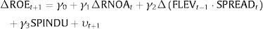
Suppose now that Eq. (2) is misspecified because the next-year profitability depends on the contextual setting with a significantly different contribution. In our first group of hypotheses, we test for the incremental information content of contextual information by expanding the autoregressive model in the following way.
where SPINDU=ROEt−ROE¯tINDUSTRYStDevtROE¯tINDUSTRY,ROE¯tINDUSTRY is the average ROE in the industry, per year and country, and StDevtROE¯tINDUSTRY is the standard deviation of the average ROE in the industry, per year and country. If we consider levels of profitability, instead of changes, in the autoregressive expanded equation, we get the following equation:

Using these models, we test whether the relative position of the firm's profitability with respect to the industry average levels of profitability adds useful information to the estimation of the next-year levels and changes of profitability (H1a and H1b).
For example, a positive value of the industry spread variable can indicate a better firm position either with negative or positive ROEs, that is, it could come from a not so bad performance of a firm inside a bad industry or from a better performance inside a good industry. Eqs. (3) and (4) examine the information conveyed by industry spreads, but as specific patterns of profitability can be differentially informative, we consider them in our analyses by partitioning the spread variable into six continuous SPINDU variables as follows:
- 1.
SPINDUD_1: firm's ROE≥Industry ROE≥0. Takes the value of the spread when profitability is more positive or equal in the firm than in the industry (0 otherwise).
- 2.
SPINDUD_2: ROE≥0>Industry ROE. Takes the value of the spread when profitability is positive or zero in the firm and negative in the industry (0 otherwise).
- 3.
SPINDUD_3: 0>firm's ROE>Industry ROE. Takes the value of the spread when profitability is less negative in the firm than in the industry (0 otherwise).
- 4.
SPINDUD_4: 0≤firm's ROE<Industry ROE. Takes the value of the spread when profitability is more positive in the industry than in the firm (0 otherwise).
- 5.
SPINDUD_5: firm's ROE<0≤Industry ROE. Takes the value of the spread when profitability is positive or zero in the industry and negative in the firm (0 otherwise).
- 6.
SPINDUD_6: firm's ROE≤Industry ROE<0. Takes the value of the spread when profitability is less or equal negative in the industry than in the firm (0 otherwise).
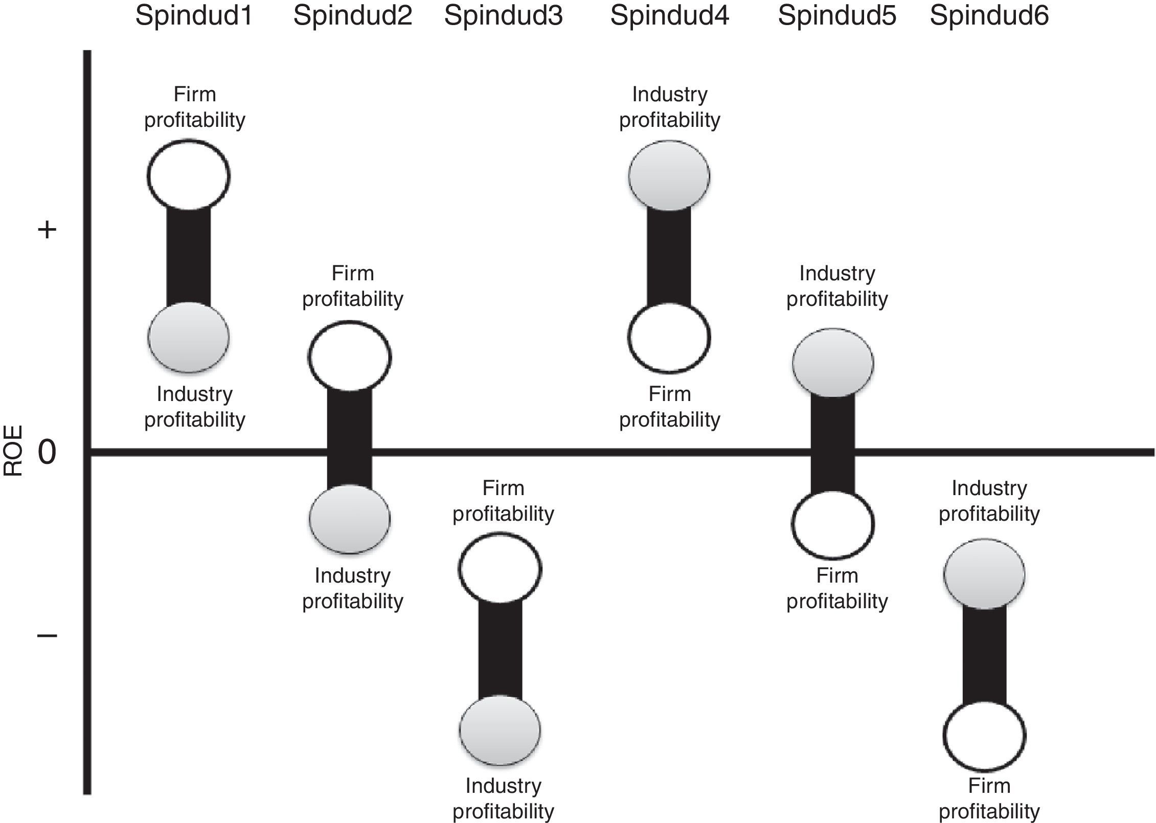
Thus, the sum of the six SPINDUD_k partitions equals SPINDU. In each partition, we measure the difference between the firm's profitability and the average value of its industry profitability, scaled by the standard deviation of the industry profitability. The first three partitions capture firms with ROEs above their industries (“good positioned” firms) while the last three partitions capture firms with ROEs below their industry averages (“bad positioned” firms), differing the partitions in terms of the signs of ROEs and spreads (Fig. 1). Therefore, we include these six partitions of SPINDU in Eqs. (3) and (4) in order to examine the information the partitions convey.
 is the difference between the firm's ROE and their Industry average value of ROE, deflacted by the standard deviation of the industry ROE, per country and year; SPINDUD_1 takes the value of the industry spread if firm's ROE≥Industry ROE≥0, and 0 otherwise; SPINDUD_2 takes the value of the industry spread if firm's ROE≥0>Industry ROE, and 0 otherwise; SPINDUD_3 takes the value of the industry spread if 0>firm's ROE>Industry ROE, and 0 otherwise; SPINDUD_4 takes the value of the industry spread if 0≤firm's ROE<Industry ROE, and 0 otherwise; SPINDUD_5 takes the value of the industry spread if firm's ROE<0≤Industry ROE, and 0 otherwise; SPINDUD_6 takes the value of the industry spread if firm's ROE≤Industry ROE<0, and 0 otherwise.")
Meaning of SPINDUD variables. Notes: SPINDU (Industry Spread) is the difference between the firm's ROE and their Industry average value of ROE, deflacted by the standard deviation of the industry ROE, per country and year; SPINDUD_1 takes the value of the industry spread if firm's ROE≥Industry ROE≥0, and 0 otherwise; SPINDUD_2 takes the value of the industry spread if firm's ROE≥0>Industry ROE, and 0 otherwise; SPINDUD_3 takes the value of the industry spread if 0>firm's ROE>Industry ROE, and 0 otherwise; SPINDUD_4 takes the value of the industry spread if 0≤firm's ROE<Industry ROE, and 0 otherwise; SPINDUD_5 takes the value of the industry spread if firm's ROE<0≤Industry ROE, and 0 otherwise; SPINDUD_6 takes the value of the industry spread if firm's ROE≤Industry ROE<0, and 0 otherwise.
After testing the incremental information of the contextual approach when using the overall measure of ROE, we test whether the disaggregation into its operating and financing components provides incremental information content for predicting future profitability, following a similar pattern (H2a and H2b). Eq. (5) looks at ROE as driven by the return on operating activities with an additional contribution from the leverage of financial activities. This leverage effect is determined by the amount of leverage and the spread between the return on operating activities and the net borrowing costs. Substituting Eq. (1) in Eq. (3) and Eq. (4), we have:
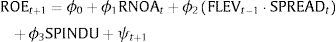
where RNOA is Return on Net Operating Assets (Operating Income/Net Operating Assets); FLEV is Financial Leverage (Net Financial Obligations/Book Value of Common Equity); SPREAD is the difference between RNOA and Net Borrowing Cost (Net Financial Expense/Net Financial Obligations); SPINDU is the difference between the firm's ROE and their industry's average ROE, deflacted by the standard deviation of the average ROE in the industry, per country and year.
A positive RNOA indicates both PM and ATO positive or negative, and the same is true in the case of the product FLEV SPREAD, and their individual signs. Models in Eqs. (5) and (6) examine the information conveyed by RNOA and FLEV SPREAD. However, as specific patterns of signs can be differentially informative, we consider them in our analyses. To avoid the problem of mixed signs, we take RNOAs and FLEV SPREAD and apply partitions to disaggregate them into four continuous variables according to their drivers’ signs (PM and ATO in one case, and FLEV and SPREAD in the other). The sum of the four RNOA_k partitions equals RNOA, and the sum of the four FLEV SPREAD_k equals FLEV SPREAD. Partitions 1 and 4 capture firms with both signs equal (positive and negative, respectively), partition 2 captures firms with positive variable first and negative second, and partition 3 captures firms with negative variable first and positive second. Therefore, we add these partitions in eq. 5 and 6 in order to test the information the new partitions convey.
Sample and descriptive analysisSampleFrom the Worldscope database we take all firms from the UK, Germany, France and Spain (45,832 firm-year observations) with the required data for years t−1, t, and t+1, from 1981 to 2008. In order to avoid the effects of outliers, we winsorize all variables at the bottom and top 3% of their distributions. All firm-year observations with SIC codes 6000–6999 (financial companies) are excluded because the operating-financing decomposition is not meaningful for these firms. This is consistent with previous studies on the DuPont analysis (Fairfield & Yohn, 2001; Nissim & Penman, 2001; Soliman, 2008) and thereby facilitates comparison among studies.
We follow the identification of operating and financing items proposed4 by Nissim and Penman (2001). To compute industries, we follow a standard approach in the literature. Fama and French (1997) start from firms’ 4-digit SIC codes and reorganize them into 48 industry groupings5 to illustrate the cost of equity at industry level. More recently the number of industries has been expanded to 49. Our analysis is based on this FF 49 industry definitions based on SIC codes, though the four industries made up of financial or real estate firms have been dropped.
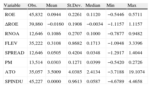
Descriptive statisticsTable 1 reports the descriptive statistics. Mean and Median ROE values are hovering around 10% in the total sample. If we focus on specific countries (untabulated results), firms in Germany are less profitable than in the rest of the countries. In contrast, Spain shows the highest mean, whereas the UK displays the highest median and dispersion. The mean change in ROE is negative, with a wide range, indicating the ROE tendency to decrease during the sample period.
Descriptive statistics. Main variables.
| Variable | Obs. | Mean | St.Dev. | Median | Min | Max |
| ROE | 45,832 | 0.0944 | 0.2261 | 0.1120 | −0.5446 | 0.5711 |
| ΔROE | 39,860 | −0.0160 | 0.1908 | −0.0034 | −1.1157 | 1.1157 |
| RNOA | 12,646 | 0.1086 | 0.2707 | 0.1000 | −0.7877 | 0.9482 |
| FLEV | 35,222 | 0.3108 | 0.8682 | 0.1713 | −1.0948 | 3.3396 |
| SPREAD | 12,646 | 0.0505 | 0.4204 | 0.0348 | −1.2917 | 1.4044 |
| PM | 13,514 | 0.0303 | 0.1271 | 0.0399 | −0.5420 | 0.2726 |
| ATO | 35,057 | 3.5009 | 4.0385 | 2.4134 | −3.7188 | 19.1074 |
| SPINDU | 45,227 | 0.0000 | 0.9613 | 0.0587 | −4.6789 | 4.4658 |
Notes: ROE is Return on Equity; ΔROE is the change of ROE; RNOA is Return on Net Operating Assets (Operating Income/Net Operating Assets); FLEV is Financial Leverage (Net Financial Obligations/Book value of common equity); SPREAD is the difference between RNOA and Net Borrowing Cost (Net Financial Expense/Net Financial Obligations); PM is the Profit Margin (Operating Income/Sales); ATO is the Asset Turnover (Sales/Net Operating Assets); SPINDU is the firm's ROE minus the Industry's average value of ROE per country and year, deflacted by the standard deviation of industry ROE.
If we focus on the operating performance, RNOA displays mean and median values above ROE, but with greater dispersion. In other words, operating activities return tends to be higher than the overall ROE, due to the effect of financial activities. The average profit margin is around 3%, with more margin (but less asset turnovers) in Spain and the UK, and less margin (but more asset turnovers) in Germany and France.
Looking at the financial activities, Spanish firms are more leveraged than the rest, with an average value of 0.54 for Net Financial Obligations per unit of Equity. On the contrary, firms in the UK have less Net Financial Obligations in their balance sheets. Spreads are positive, that is, operating activities add value to the overall ROE. Considering the entire sample, on average, operating activities generate a 5% over the Net Borrowing Costs.
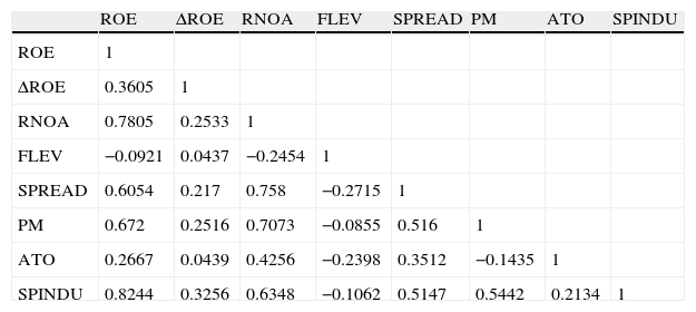
Table 2 provides the correlations between variables. ROE, RNOA, SPREAD, PM and SPINDU are highly correlated, indicating that most profitability comes from the firm operating activities and from the industry spread. Furthermore, Profit Margins and the difference between operating performance and Net Borrowing Costs seem to drive operating profitability. Leverage signs are consistent with a negative influence of indebtedness in profitability (both RNOA and ROE) which seems to be originated in a reduction of the spread of rates.
Correlation analysis.
| ROE | ΔROE | RNOA | FLEV | SPREAD | PM | ATO | SPINDU | |
| ROE | 1 | |||||||
| ΔROE | 0.3605 | 1 | ||||||
| RNOA | 0.7805 | 0.2533 | 1 | |||||
| FLEV | −0.0921 | 0.0437 | −0.2454 | 1 | ||||
| SPREAD | 0.6054 | 0.217 | 0.758 | −0.2715 | 1 | |||
| PM | 0.672 | 0.2516 | 0.7073 | −0.0855 | 0.516 | 1 | ||
| ATO | 0.2667 | 0.0439 | 0.4256 | −0.2398 | 0.3512 | −0.1435 | 1 | |
| SPINDU | 0.8244 | 0.3256 | 0.6348 | −0.1062 | 0.5147 | 0.5442 | 0.2134 | 1 |
Notes: ROE is Return on Equity; ΔROE is the change of ROE; RNOA is Return on Net Operating Assets (Operating Income/Net Operating Assets); FLEV is Financial Leverage (Net Financial Obligations/Book value of common equity); SPREAD is the difference between RNOA and Net Borrowing Cost (Net Financial Expense/Net Financial Obligations); PM is the Profit Margin (Operating Income/Sales); ATO is the Asset Turnover (Sales/Net Operating Assets); SPINDU is the firm's ROE minus the Industry's average value of ROE per country and year, deflacted by the standard deviation of industry ROE.
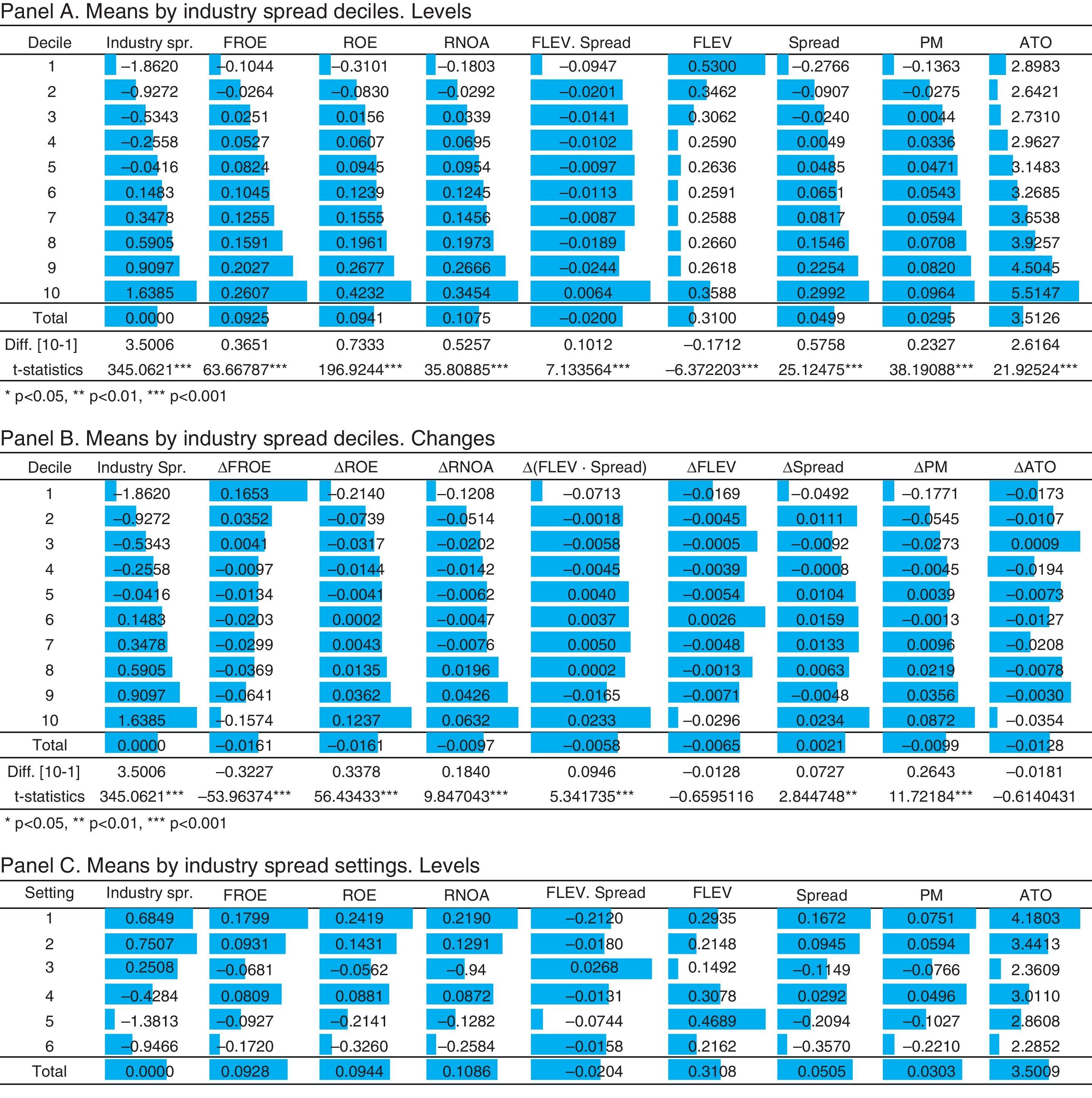
In order to determine the nature of relations between industry spread, and ROE and its first-level and second-level drivers, using the drivers obtained by Nissim and Penman's (2001) disaggregation, we have divided our sample in deciles. This approach6 has the advantage of providing a simple picture of how average variables (future and current ROE and its operating and financing drivers) vary across the spectrum of the industry profitability spread, helping us to decide the fair level of disaggregation of the explanatory variables in subsequent Fama and MacBeth regression analysis. Figure 2, Panel A shows the mean values for the variables used, classified by Industry Spread deciles, and non-lineal relations can be graphically appreciated.
; FLEV is Financial Leverage (Net Financial Obligations/Book value of common equity); SPREAD is the difference between RNOA and Net Borrowing Cost (Net Financial Expense/Net Financial Obligations); PM is the Profit Margin (Operating Income/Sales); ATO is the Asset Turnover (Sales/Net Operating Assets). In Panel C, Settings are the six industry spread categories, explained in Fig. 1.")
Portfolios of Industry Spread Deciles. Notes: ROE is Return on Equity; ΔROE is the change of ROE; Industry Spread is the difference between the firm's ROE and their Industry's average ROE, per country and year, deflacted by the standard deviation of industry ROE; FROE is ROE of t+1; RNOA is Return on Net Operating Assets (Operating Income/Net Operating Assets); FLEV is Financial Leverage (Net Financial Obligations/Book value of common equity); SPREAD is the difference between RNOA and Net Borrowing Cost (Net Financial Expense/Net Financial Obligations); PM is the Profit Margin (Operating Income/Sales); ATO is the Asset Turnover (Sales/Net Operating Assets). In Panel C, Settings are the six industry spread categories, explained in Fig. 1.
As the industry spread is higher, the next-year ROE and current ROE progressively increase. Looking at the disaggregation of ROE into RNOA and FLEV·SPREAD, we can see that RNOA raises, while FLEV·SPREAD does not show a clear pattern, though the strong negative mean value of this product, FLEV·SPREAD, can be emphasized for the first-decile firms, the ones with the higher industry spread. In order to analyze the financial factor in depth, we break down the product into its two components. Thus, we find that FLEV tends to decrease as the industry spread grows, though the decrease is not fully lineal. For the first decile, FLEV is higher, indicating that less profitable firms, with respect to the industry level, have the highest debt. From decile 2 FLEV decreases gradually up to decile 9, in which the FLEV mean value is the minimum (0.25), but the decile 10 shows a light increase.
SPREAD shows a growing pattern: it has a negative mean value for deciles 1 to 3, for which RNOA is negative or very small. As SPREAD is the difference between RNOA and NBC, the firm has to get an operative return higher than NBC for SPREAD to be positive.
If we now focus in the disaggregation of RNOA, we observe that both PM and ATO show a growing trend, across the deciles, even though it is more pronounced for ATO. The negative operating profitability seems to be induced by a negative profit margin; and ATO acts as a multiplier, increasing the differences of RNOA among deciles.
Panel B shows the mean values of changes in ROE and its drivers by industry spread deciles. Similar to in the previous analysis by levels, as the industry spread grows, changes in current ROE increase progressively. On the other hand, changes in the next-year ROE progressively decrease, showing a reversion pattern with respect to industry profitability.
Looking at the disaggregation of the changes in ROE into changes of RNOA and the changes of FLEV·SPREAD, we find a similar behavior in levels. Changes in RNOA grow, while changes in FLEV·SPREAD do not show a clear pattern. Again, the strong negative contribution of FLEV·SPREAD for the first decile is remarkable. If we break down changes in FLEV·SPREAD into its two components, we cannot see a trend in the changes of FLEV, though changes in SPREAD show an irregular growing trend. As for the components of the changes in RNOA, PM shows a growing trend, while ATO pattern is not regular.
Panel C shows the behavior of the variables according to the relative position of the firm-specific ROE respect to the industry ROE (vid. Fig. 1). In the first three settings (SPINDUD_1–3), the firm's ROE is higher than the industry mean value of ROE, while the opposite occurs in the other three settings (SPINDUD_4–6). As a whole, it can be noted that for SPINDUD_1–3, as the industry profitability is lower, progressive decrease is found in the firm's profitability, computed both as current ROE and the next-year ROE, as well as in their drivers: RNOA, FLEV, SPREAD, PM and ATO. A similar pattern can be observed for SPINDUD_4–6, except for FLEV. This classification supports the idea of a non-linear behavior of the firm's financial leverage.
We disaggregate the firm-specific industry spread, into six variables according to signs and relative positions, each one being a continuous variable that takes the value of SPINDU if signs and firm position are the selected for the group, and 0 otherwise, as described in Fig. 1. This way, we can appreciate if the relative position of firms’ profitability in respect to their industry's and the respective signs mean differential effects on future profitability. For the variables SPINDUD_1, SPINDUD_2 and SPINDUD_4, in which the firm profitability is positive, the mean values of RNOA and PM are positive too. For SPINDUD_3, SPINDUD_5 and SPINDUD_6, in which the firm profitability is negative, the mean values of RNOA and PM show the same sign. These results point out to RNOA as the main driver of ROE, and PM as the main driver of RNOA.
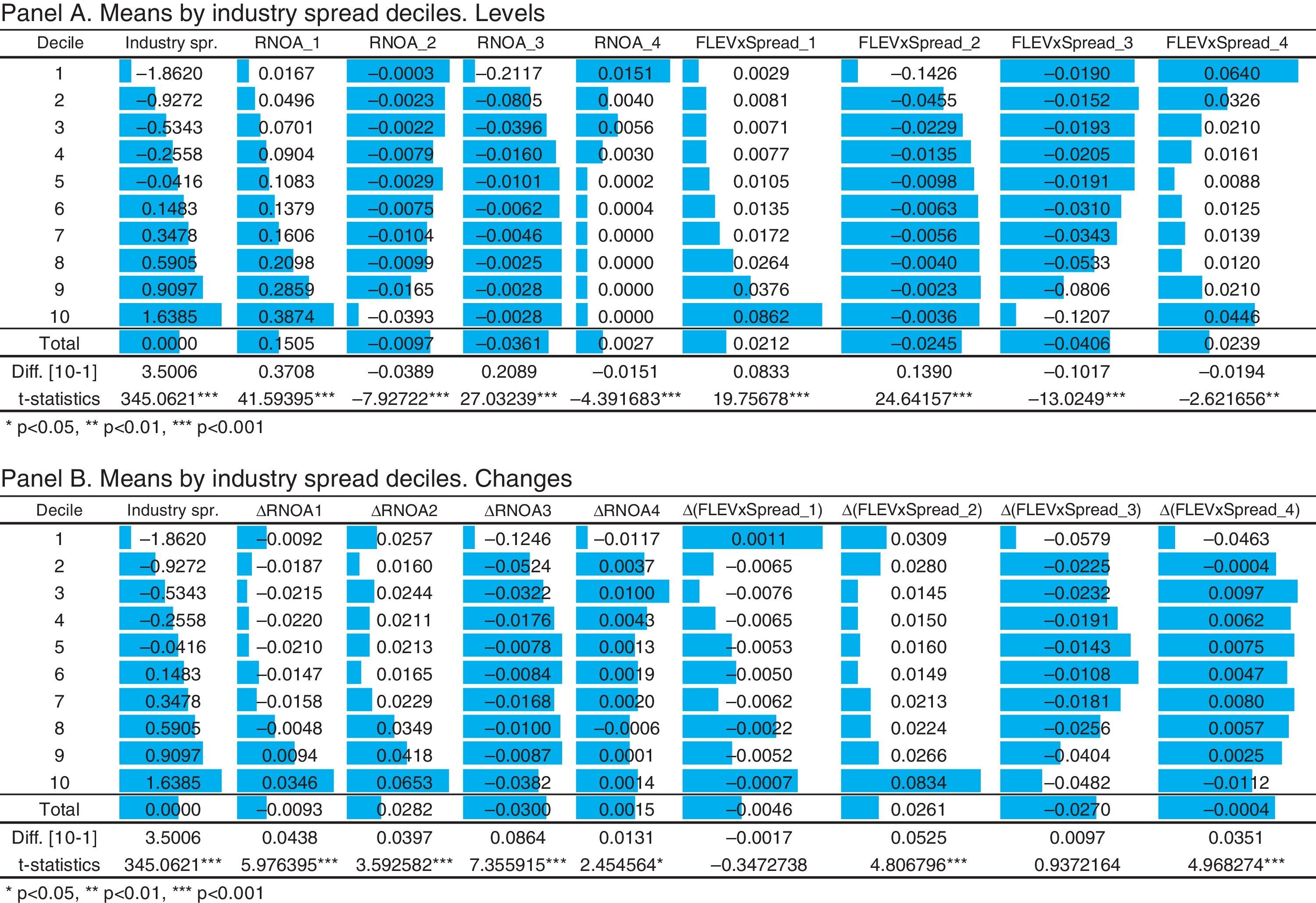
Fig. 3 shows a further disaggregation of that information contained in Fig. 2. Each variable, RNOA and FLEV·SPREAD, is broken down into four new variables, according to the signs of the respective drivers (PM and ATO; FLEV and SPREAD).
Unlike previous ROE and RNOA analyses, in which only positive signs are taken, considerably reducing samples and introducing a clear bias toward the best companies, our study uses disaggregation by signs in order to identify potential different patterns in each case. The proposed methodology outperforms those previously used in the literature in terms of the completion of the selected sample by avoiding the interpretation difficulties originated from the interaction of different signs in ratio variables (Fig. 3).
; FLEV is Financial Leverage (Net Financial Obligations/Book value of common equity); SPREAD is the difference between RNOA and Net Borrowing Cost (Net Financial Expense/Net Financial Obligations); PM is the Profit Margin (Operating Income/Sales); ATO is the Asset Turnover (Sales/Net Operating Assets); RNOA_1 takes the value of RNOA if PM>0 and ATO>0, and 0 otherwise; RNOA_2 takes the value of RNOA if PM>0 and ATO<0, and 0 otherwise; RNOA_3 takes the value of RNOA if PM<0 and ATO>0, and 0 otherwise; RNOA_4 takes the value of RNOA if PM<0 and ATO<0, and 0 otherwise; FLEV·SPREAD_1 takes the value of FLEV·SPREAD if FLEV>0 and SPREAD >0, and 0 otherwise; FLEV·SPREAD_2 takes the value of FLEV·SPREAD if FLEV>0 and SPREAD <0, and 0 otherwise; FLEV·SPREAD_3 takes the value of FLEV·SPREAD if FLEV<0 and SPREAD >0, and 0 otherwise; FLEV·SPREAD_4 takes the value of FLEV·SPREAD if FLEV<0 and SPREAD <0, and 0 otherwise.")
Portfolios of Industry Spread Deciles. Disaggregated Variables. Notes: Industry Spread is the difference between the firm's ROE and their Industry's average ROE, per country and year, deflacted by the standard deviation of industry ROE; RNOA is Return on Net Operating Assets (Operating Income/Net Operating Assets); FLEV is Financial Leverage (Net Financial Obligations/Book value of common equity); SPREAD is the difference between RNOA and Net Borrowing Cost (Net Financial Expense/Net Financial Obligations); PM is the Profit Margin (Operating Income/Sales); ATO is the Asset Turnover (Sales/Net Operating Assets); RNOA_1 takes the value of RNOA if PM>0 and ATO>0, and 0 otherwise; RNOA_2 takes the value of RNOA if PM>0 and ATO<0, and 0 otherwise; RNOA_3 takes the value of RNOA if PM<0 and ATO>0, and 0 otherwise; RNOA_4 takes the value of RNOA if PM<0 and ATO<0, and 0 otherwise; FLEV·SPREAD_1 takes the value of FLEV·SPREAD if FLEV>0 and SPREAD >0, and 0 otherwise; FLEV·SPREAD_2 takes the value of FLEV·SPREAD if FLEV>0 and SPREAD <0, and 0 otherwise; FLEV·SPREAD_3 takes the value of FLEV·SPREAD if FLEV<0 and SPREAD >0, and 0 otherwise; FLEV·SPREAD_4 takes the value of FLEV·SPREAD if FLEV<0 and SPREAD <0, and 0 otherwise.
As for the first variable, RNOA, when both PM and ATO are positive (RNOA_1), RNOA gradually grows as the industry spread increases, but just the opposite pattern can be seen when both PM and ATO are negative (RNOA_4). For RNOA_2 and RNOA_3 the shift pattern is gentler, except in the extreme decile with lower values. When PM is positive and ATO is negative (RNOA_2), the higher the industrial spread, the lower the RNOA, and, the opposite evolution of mean values is found when PM is negative and ATO is positive (RNOA_3).
Concerning the second variable, FLEV·SPREAD, when FLEV is positive (FLEV·SPREAD_1 y FLEV·SPREAD_2), the product FLEV·SPREAD grows as the firm profitability exceeds the industry one. A positive SPREAD increases differences across deciles, while a negative SPREAD results in a gentler growth pattern. For FLEV·SPREAD_3 (negative FLEV and positive SPREAD) an opposite pattern to that for FLEV·SPREAD_2 is found: a gentle negative trend. However, when both FLEV and SPREAD are negative, a U-pattern is found. Negative industry spread, where negative firm profitability is higher than negative industry profitability, induces lower levels of FLEV·SPREAD as the negative difference decreases, while positive industry spread, meaning higher negative profitability in the industry than in the firm, induces growing FLEV·SPREAD as the positive difference increases. A clear non-linear relation is suggested between the industry spread and the financial driver, FLEV·SPREAD, when both components are negative.
Panel B shows changes in variables by deciles of profitability spread between the firms’ values and their industries’ mean values. Non-linear relations can be appreciated in RNOA and FLEV·SPREAD for any combinations of signs of the drivers they are made up of. Specifically, values display a U-pattern with minimums around zero industry spread for RNOA2 (PM>0; ATO<0) and FLEV·SPREAD2 (FLEV>0; SPREAD<0), and the opposite shape, with maximum values around zero industry spread for RNOA3 (PM<0; ATO>0) and FLEV·SPREAD3 (FLEV<0; SPREAD>0).
ResultsIn this section, we document the incremental information added by the firms’ position in their industry. We start with profitability levels. Then, we develop the same type of analysis considering ROE changes. After having disaggregated ROE in its first-level drivers in the presence of contextual information, we perform a third group of regressions. Using the disaggregation of the operating and financing ROE drivers into four variables each, according to the signs of their second-level drivers, we run a fourth group of regressions. Finally, we test how firms’ size conditions our previous results.
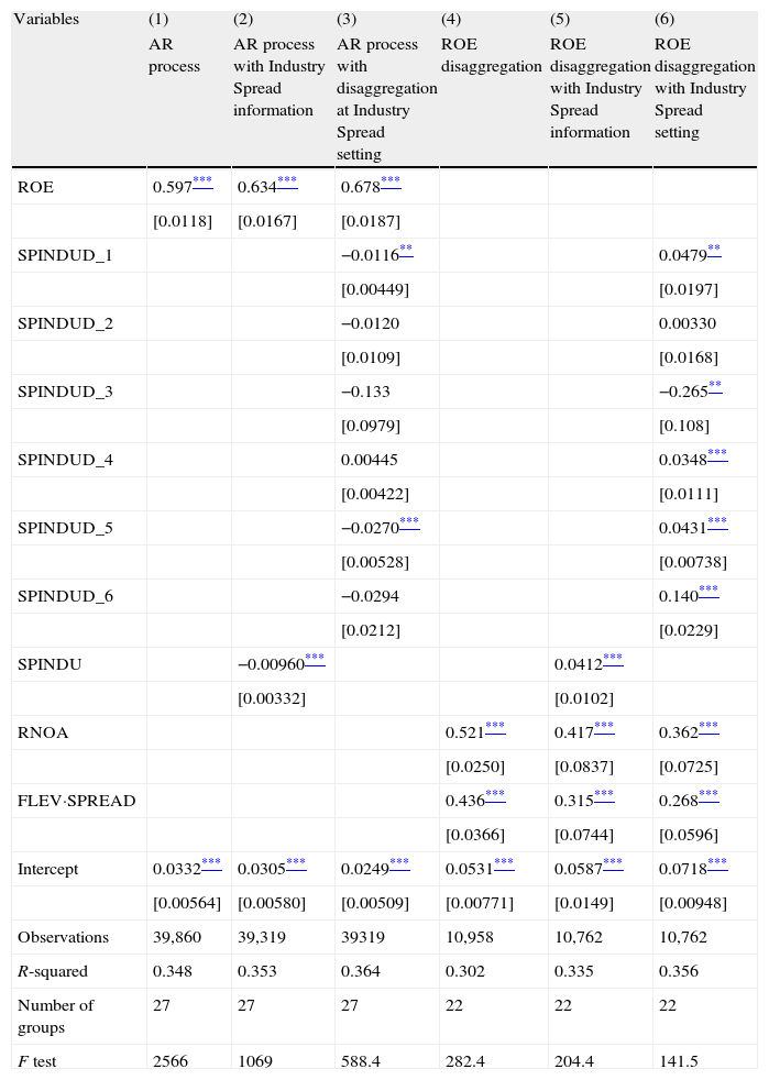
Estimation of ROE levels and changes in the presence of contextual informationIn the previous evidence section we hypothesize that the relative position of the firm's profitability with respect to the industry average profitability adds information to the estimation of the next-year ROE (H1a). To test this hypothesis we employ Eq. (4) and the regression results are displayed in Table 3, column 2.
Fama–MacBeth two-step procedure. All Sample. Dependent: ROEt+1.
| Variables | (1) | (2) | (3) | (4) | (5) | (6) |
| AR process | AR process with Industry Spread information | AR process with disaggregation at Industry Spread setting | ROE disaggregation | ROE disaggregation with Industry Spread information | ROE disaggregation with Industry Spread setting | |
| ROE | 0.597*** | 0.634*** | 0.678*** | |||
| [0.0118] | [0.0167] | [0.0187] | ||||
| SPINDUD_1 | −0.0116** | 0.0479** | ||||
| [0.00449] | [0.0197] | |||||
| SPINDUD_2 | −0.0120 | 0.00330 | ||||
| [0.0109] | [0.0168] | |||||
| SPINDUD_3 | −0.133 | −0.265** | ||||
| [0.0979] | [0.108] | |||||
| SPINDUD_4 | 0.00445 | 0.0348*** | ||||
| [0.00422] | [0.0111] | |||||
| SPINDUD_5 | −0.0270*** | 0.0431*** | ||||
| [0.00528] | [0.00738] | |||||
| SPINDUD_6 | −0.0294 | 0.140*** | ||||
| [0.0212] | [0.0229] | |||||
| SPINDU | −0.00960*** | 0.0412*** | ||||
| [0.00332] | [0.0102] | |||||
| RNOA | 0.521*** | 0.417*** | 0.362*** | |||
| [0.0250] | [0.0837] | [0.0725] | ||||
| FLEV·SPREAD | 0.436*** | 0.315*** | 0.268*** | |||
| [0.0366] | [0.0744] | [0.0596] | ||||
| Intercept | 0.0332*** | 0.0305*** | 0.0249*** | 0.0531*** | 0.0587*** | 0.0718*** |
| [0.00564] | [0.00580] | [0.00509] | [0.00771] | [0.0149] | [0.00948] | |
| Observations | 39,860 | 39,319 | 39319 | 10,958 | 10,762 | 10,762 |
| R-squared | 0.348 | 0.353 | 0.364 | 0.302 | 0.335 | 0.356 |
| Number of groups | 27 | 27 | 27 | 22 | 22 | 22 |
| F test | 2566 | 1069 | 588.4 | 282.4 | 204.4 | 141.5 |
Standard errors in brackets.
Notes: ROE is the Return On Equity; SPINDU is the firm's ROE minus the Industry's average value of ROE per country and year, deflacted by the standard deviation of industry ROE; RNOA is Return on Net Operating Assets (Operating Income/Net Operating Assets); FLEV is Financial Leverage (Net Financial Obligations/Book value of common equity); SPREAD is the difference between RNOA and Net Borrowing Cost (Net Financial Expense/Net Financial Obligations); SPINDUD_1 takes the value of the industry spread if firm's ROE≥Industry ROE≥0, and 0 otherwise; SPINDUD_2 takes the value of the industry spread if firm's ROE≥0>Industry ROE, and 0 otherwise; SPINDUD_3 takes the value of the industry spread if 0>firm's ROE>Industry ROE, and 0 otherwise; SPINDUD_4 takes the value of the industry spread if 0≤firm's ROE<Industry ROE, and 0 otherwise; SPINDUD_5 takes the value of the industry spread if firm's ROE<0≤Industry ROE, and 0 otherwise; SPINDUD_6 takes the value of the industry spread if firm's ROE ≤ Industry ROE<0, and 0 otherwise.
*p<0.1.
Considering the autoregressive process only (column 1), ROE has a persistence of 0.60. However, when industry information is included through a variable measuring the difference between each firm's ROE and its industry's average value of ROE (column 2), the coefficient of this new variable is negative, and ROE persistence increases to 0.63. This means that firms whose ROE is above the industry average tend to be less profitable in the next period, while firms whose ROE is below the industry average, tend to be more profitable in the next period.
In order to identify the nature of the reversal pattern more precisely, we have run the model after disaggregating the variable industry spread (SPINDU) into 6 variables, according to the signs and the relative positions of the firms’ profitability and the mean values of their industries’ profitability.7 As expected, after performing the portfolio analysis, when the firm's profitability is higher than the industries’, there is a reversion pattern to reduce future ROE, though it is considerably lower for negative industries’ profitability. On the contrary, when the firms’ profitability is negative and lower than their industry's profitability, the reversion pattern to make ROE less negative is stronger, consistent with Fama and French's (2000) results. Besides, the intercept value decreases as we incorporate the general industry spread variable, and even more when this variable is disaggregated. This would indicate that a higher part of the dependent variable is explained by the independent variables included in the model. At the same time, the improvement in R2 shows a higher explanatory power.
Our results expand those concerning the regression toward the mean values of ROE obtained by Freeman et al. (1982), by conditioning this regression to the relative position of the firms’ and their industries’ profitability, which has proved to be determinant in defining some non-linearities of the reversals.
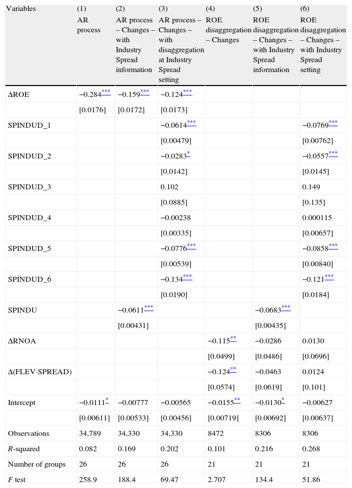
Now, we perform the same type of analysis, but considering changes in profitability (H1b). Table 4 reports the incremental information content of adding industry-level relative profitability metrics for predicting the next-year changes of ROE.
Profitability changes. Fama–MacBeth two-step procedure. All Sample. Dependent: Change in ROE t+1.
| Variables | (1) | (2) | (3) | (4) | (5) | (6) |
| AR process | AR process – Changes – with Industry Spread information | AR process – Changes – with disaggregation at Industry Spread setting | ROE disaggregation – Changes | ROE disaggregation – Changes – with Industry Spread information | ROE disaggregation – Changes – with Industry Spread setting | |
| ΔROE | −0.284*** | −0.159*** | −0.124*** | |||
| [0.0176] | [0.0172] | [0.0173] | ||||
| SPINDUD_1 | −0.0614*** | −0.0769*** | ||||
| [0.00479] | [0.00762] | |||||
| SPINDUD_2 | −0.0283* | −0.0557*** | ||||
| [0.0142] | [0.0145] | |||||
| SPINDUD_3 | 0.102 | 0.149 | ||||
| [0.0885] | [0.135] | |||||
| SPINDUD_4 | −0.00238 | 0.000115 | ||||
| [0.00335] | [0.00657] | |||||
| SPINDUD_5 | −0.0776*** | −0.0858*** | ||||
| [0.00539] | [0.00840] | |||||
| SPINDUD_6 | −0.134*** | −0.121*** | ||||
| [0.0190] | [0.0184] | |||||
| SPINDU | −0.0611*** | −0.0683*** | ||||
| [0.00431] | [0.00435] | |||||
| ΔRNOA | −0.115** | −0.0286 | 0.0130 | |||
| [0.0499] | [0.0486] | [0.0696] | ||||
| Δ(FLEV·SPREAD) | −0.124** | −0.0463 | 0.0124 | |||
| [0.0574] | [0.0619] | [0.101] | ||||
| Intercept | −0.0111* | −0.00777 | −0.00565 | −0.0155** | −0.0130* | −0.00627 |
| [0.00611] | [0.00533] | [0.00456] | [0.00719] | [0.00692] | [0.00637] | |
| Observations | 34,789 | 34,330 | 34,330 | 8472 | 8306 | 8306 |
| R-squared | 0.082 | 0.169 | 0.202 | 0.101 | 0.216 | 0.268 |
| Number of groups | 26 | 26 | 26 | 21 | 21 | 21 |
| F test | 258.9 | 188.4 | 69.47 | 2.707 | 134.4 | 51.86 |
Standard errors in brackets.
Notes: ΔROE is the change of Return On Equity; SPINDU is the difference between the firm's ROE and their industry average value of ROE, per country and year; deflacted by the standard deviation of industry ROE; ΔRNOA is the change of Return on Net Operating Assets (Operating Income/Net Operating Assets); FLEV is Financial Leverage (Net Financial Obligations/Book value of common equity); SPREAD is the difference between RNOA and Net Borrowing Cost (Net Financial Expense/Net Financial Obligations); SPINDUD_1 takes the value of the industry spread if firm's ROE≥Industry ROE≥0, and 0 otherwise; SPINDUD_2 takes the value of the industry spread if firm's ROE≥0>Industry ROE, and 0 otherwise; SPINDUD_3 takes the value of the industry spread if 0>firm's ROE>Industry ROE, and 0 otherwise; SPINDUD_4 takes the value of the industry spread if 0≤firm's ROE<Industry ROE, and 0 otherwise; SPINDUD_5 takes the value of the industry spread if firm's ROE<0≤Industry ROE, and 0 otherwise; SPINDUD_6 takes the value of the industry spread if firm's ROE≤Industry ROE<0, and 0 otherwise.
We find that changes in ROE imply mean reversion, and this is consistent with our results for profitability levels displayed in Table 3, in which the coefficient of current ROE was lower than 1, and the relative situation of the firm in respect to the industry showed a reversion pattern. Considering the autoregressive process of profitability information alone (Table 4, column 1), the coefficient indicates that the current-year positive (negative) variation of profitability reverts to a reduction (increase) of 28% in the subsequent year. However, the reversal component is attenuated to just 16% when the industry-relative factor is incorporated. Column (2) shows that differences between specific firms and the whole industry suffer a strong reversal. Firms which are more profitable than the industry average tend to reduce the next-year ROE changes. In turn, firms less profitable than the industry average tend to benefit from positive changes in ROE. After disaggregating the variable industry spread (SPINDU) into 6 variables (column 3) results are similar to those for profitability levels, that is, the reversion effect of differences in profitability showed in ROE coefficients decreases even more. In addition, after adding the contextual factors the intercept is not even significant, suggesting that the variables included get a good specification of the model; at the same time, R2 is more than double when the industry-relative variable is added, and a better R2 is obtained when the industry variable is disaggregated, indicating an improved explanatory power of the model. As in levels, the reversion pattern due to the industry effect is stronger in firms with negative profitability when the industry mean value of ROE is higher (positive or less negative). Also, a clear reversion effect is identified when the firms’ profitability is positive and higher than mean value of the industry profitability.
These results confirm our hypothesis H1b. In the estimation of the next-year ΔROE, not only is the historical change in profitability needed, but also the status of the firm's ROE compared to the industry average, both factors inducing profitability reversals. Furthermore, the relative position of firm's profitability in respect to the industry benchmark determines the reversion speed: negative firms’ profitability, when the industry's mean value of ROE is higher (either positive or less negative), induces the strongest reversion patterns; then, positive firms’ profitability higher than the positive industry benchmark induces reversion patters similar to those obtained with the model including a comprehensive industry-relative variable; for SPINDUD_2, gathering firms with positive profitability when the industry benchmark is negative, the reversion pattern is weaker; and finally, no significant reversion pattern is found for SPINDUD_3 (negative firm's profitability and more negative industry's profitability) and SPINDUD_4 (positive firm's profitability lower than industry's profitability). This way, our results support those of Fama and French (2000) on non-linear behavior of changes of profitability and extend them by a better specification of the extremes.
Disaggregating ROE in the presence of contextual informationTo test our second group of hypotheses we substitute contemporaneous ROE by the breakdown into RNOA and FLEV·SPREAD. Therefore, we test whether the levels of RNOA, FLEV·SPREAD, and the industry-relative profitability factor provide incremental information content for predicting profitability in terms of the next-year ROE.
Table 3, column 4, shows that the current levels of RNOA and the product FLEV·SPREAD significantly contribute to explain the subsequent ROE. However, the coefficients considerably decrease if we incorporate the relative profitability of the firm with respect to the industry average value (column 5), and this factor contributes positively to explain the next-year ROE.
Comparing columns 1–3 with columns 4–6, we realize that many less firms are included in the latter as the computing of those variables in Table 3 is more demanding in data. When we decompose current ROE into its first-level drivers, RNOA and FLEV·SPREAD, intercept increases, what this could mean is that these two variables behave in a less linear pattern than ROE. Therefore, when we introduce the industry-relative factor, its coefficient shows a positive contribution over the other two variables to explain the next-year ROE, instead of reflecting a reversion pattern as in the first three columns. In the same line, after disaggregating the comprehensive industry-relative factor into 6 factors, according to signs and relative positions of profitability, their contribution to the next-year ROE shows contrary signs when significant. In role of industry spread in future profitability by firm size section we extend these results by separately analyzing different sizes of firms.
We also test whether disaggregating the current change in ROE (ΔROE) into the change in RNOA (ΔRNOA) and the change in FLEV·SPREAD (ΔFLEV·SPREAD) provides additional information to forecast the next-year change of ROE. In Table 4, columns 4–6, we report regressions run by using Eq. (5).
We find that the change in RNOA and the change in the product FLEV·SPREAD show a negative contribution to the next-year change in ROE. If we incorporate industry-based relative information (column 5), current ΔRNOA and ΔFLEV·SPREAD are no more significant to predict the next-year change in ROE. The industry factor seems to be a better source of information to estimate reversals in profitability changes (coefficient=−0.07). As in this case changes in the first-level drivers of ROE are not significant to explain the next-year changes in ROE, the disaggregated industry-relative factors show similar reversion patterns (col. 6) than using ROE as explanatory variable (col. 3).
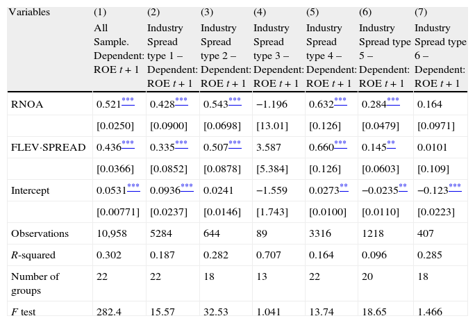
Disaggregation of ROE drivers by signs in industry spread settingsIn order to describe the effect more accurately, we have run our model with RNOA and FLEV·SPREAD as explanatory variables for the six different settings of industry spread, according to the signs and the relative position of the firm's profitability and the industry's mean value of profitability. Results are shown in Table 5. Non-significant coefficients appear just in those groups with a fewer number of observations (industry spread types 3 and 6, columns 4 and 7); hence, our significant results are focused on all firms with positive profitability, wherever the relative situation to the industry's profitability (9244 observations), and those firms with negative profitability whose industry is obtaining a positive profitability (1218 observations). In our sample, this method allows us to analyze 95% of the population (10,462 out of 10,958) instead of 84% that could be analyzed if only positive profitability were taken. But the difference increases at the second level of disaggregation. Out of 10,958 observations in our sample, only 4311 could be used if PM, ATO, FLEV and SPREAD were restricted to positive values. Therefore, the methodology used in this work lets us obtain significant results for 95% of observations in our sample, while the methods used in previous literature would have analyzed no more than 39%. Note that about half of the observations are included in the first industry spread type, in which both the firms’ profitability and their industries’ profitability is positive, the firms’ being higher. Looking at the significant coefficients, we can see that both the operating and the financing drivers of profitability are better inductors of next-year ROE when the firm is performing well but falls behind the industry's benchmark (industry spread type 4, column 5). Similarly, when the industry's profitability is not a good benchmark for the firm (negative industry's profitability and positive firm's profitability), both current individual drivers are more weighting factors in future ROE (industry spread type 2, column 3). In the most common setting (industry spread type 1, column 2), both factors are significant but the value of the intercept is higher, indicating that the next-year ROE is partially explained by other persistent factors not specified in the model. Logically, the intercept is negative in those models with firms getting negative profitability, showing partial reversion patterns. In setting 5 (column 6), we can appreciate that the explanatory power of the current operating and financing drivers on the next-year ROE is lower, and persistent reversion factors are being captured by the intercept, even though the R2 is poor.
Disaggregating ROE levels by industry spread. Fama–MacBeth two-step procedure.
| Variables | (1) | (2) | (3) | (4) | (5) | (6) | (7) |
| All Sample. Dependent: ROE t+1 | Industry Spread type 1 – Dependent: ROE t+1 | Industry Spread type 2 – Dependent: ROE t+1 | Industry Spread type 3 – Dependent: ROE t+1 | Industry Spread type 4 – Dependent: ROE t+1 | Industry Spread type 5 – Dependent: ROE t+1 | Industry Spread type 6 – Dependent: ROE t+1 | |
| RNOA | 0.521*** | 0.428*** | 0.543*** | −1.196 | 0.632*** | 0.284*** | 0.164 |
| [0.0250] | [0.0900] | [0.0698] | [13.01] | [0.126] | [0.0479] | [0.0971] | |
| FLEV·SPREAD | 0.436*** | 0.335*** | 0.507*** | 3.587 | 0.660*** | 0.145** | 0.0101 |
| [0.0366] | [0.0852] | [0.0878] | [5.384] | [0.126] | [0.0603] | [0.109] | |
| Intercept | 0.0531*** | 0.0936*** | 0.0241 | −1.559 | 0.0273** | −0.0235** | −0.123*** |
| [0.00771] | [0.0237] | [0.0146] | [1.743] | [0.0100] | [0.0110] | [0.0223] | |
| Observations | 10,958 | 5284 | 644 | 89 | 3316 | 1218 | 407 |
| R-squared | 0.302 | 0.187 | 0.282 | 0.707 | 0.164 | 0.096 | 0.285 |
| Number of groups | 22 | 22 | 18 | 13 | 22 | 20 | 18 |
| F test | 282.4 | 15.57 | 32.53 | 1.041 | 13.74 | 18.65 | 1.466 |
Standard errors in brackets.
Notes: ROE is the Return On Equity; RNOA is Return on Net Operating Assets (Operating Income/Net Operating Assets); FLEV is Financial Leverage (Net Financial Obligations/Book value of common equity); SPREAD is the difference between RNOA and Net Borrowing Cost (Net Financial Expense/Net Financial Obligations).
*p<0.1.
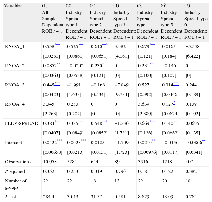
In Table 6 the same models are run, now disaggregating RNOA into the previously explained four different groups, according to the signs of its drivers, PM and ATO. The better R2 and F-tests of the model in column 1 are consistent with those results of Fairfield and Yohn (2001) about the disaggregation of RNOA into PM and ATO providing additional information for profitability forecasts. The first remarkable result is that the more common case (when both PM and ATO are positive) is behind most of comprehensive coefficients shown in Table 5. Paying attention to industry spread settings 1, 2, 4, and 5, the only exception is industry spread type 5 (col. 6) when the firm's profitability is negative but the industry's profitability is positive. In this setting, current RNOA is significant only when profit margin is negative (RNOA_3 and RNOA_4). This result supports our previous univariate analysis displayed in Figure 2 Panel C, showing equal signs for FROE, ROE, and PM. Our results support those of Amir et al. (2011) showing profit margin as a more powerful explanatory variable than asset turnover. FLEV·SPREAD coefficients maintain the same significance level and very similar coefficients than before disaggregating RNOA by signs, supporting low correlation between both drivers, as shown in Table 2.
Disaggregating ROE and RNOA levels by industry spread. Fama–MacBeth two-step procedure.
| Variables | (1) | (2) | (3) | (4) | (5) | (6) | (7) |
| All Sample. Dependent: ROE t+1 | Industry Spread type 1 – Dependent: ROE t+1 | Industry Spread type 2 – Dependent: ROE t+1 | Industry Spread type 3 – Dependent: ROE t+1 | Industry Spread type 4 – Dependent: ROE t+1 | Industry Spread type 5 – Dependent: ROE t+1 | Industry Spread type 6 – Dependent: ROE t+1 | |
| RNOA_1 | 0.558*** | 0.525*** | 0.610*** | 3.982 | 0.679*** | 0.0163 | −5.538 |
| [0.0280] | [0.0860] | [0.0651] | [4.061] | [0.121] | [0.184] | [6.422] | |
| RNOA_2 | 0.0857** | −0.0202 | 0.230* | 0 | 0.231** | −0.146 | 0 |
| [0.0363] | [0.0538] | [0.121] | [0] | [0.100] | [0.107] | [0] | |
| RNOA_3 | 0.445*** | −1.991 | −0.168 | −7.849 | 0.527 | 0.314*** | 0.244 |
| [0.0423] | [1.638] | [0.534] | [9.784] | [0.392] | [0.0446] | [0.189] | |
| RNOA_4 | 3.345 | 0.233 | 0 | 0 | 3.639 | 0.127* | 0.139 |
| [2.263] | [0.202] | [0] | [0] | [2.389] | [0.0674] | [0.192] | |
| FLEV·SPREAD | 0.384*** | 0.335*** | 0.548*** | −1.336 | 0.669*** | 0.140** | 0.0695 |
| [0.0407] | [0.0849] | [0.0852] | [1.781] | [0.126] | [0.0662] | [0.135] | |
| Intercept | 0.0422*** | 0.0628*** | 0.0125 | −1.709 | 0.0219** | −0.0156 | −0.0866** |
| [0.00658] | [0.0213] | [0.0131] | [1.723] | [0.00976] | [0.0117] | [0.0341] | |
| Observations | 10,958 | 5284 | 644 | 89 | 3316 | 1218 | 407 |
| R-squared | 0.352 | 0.253 | 0.319 | 0.796 | 0.181 | 0.122 | 0.382 |
| Number of groups | 22 | 22 | 18 | 13 | 22 | 20 | 18 |
| F test | 284.4 | 30.43 | 31.57 | 0.581 | 8.629 | 13.09 | 0.764 |
Standard errors in brackets.
Notes: ROE is the Return On Equity; RNOA is Return on Net Operating Assets (Operating Income/Net Operating Assets); FLEV is Financial Leverage (Net Financial Obligations/Book value of common equity); SPREAD is the difference between RNOA and Net Borrowing Cost (Net Financial Expense/Net Financial Obligations); RNOA_1 takes the value of RNOA if PM>0 and ATO>0, and 0 otherwise; RNOA_2 takes the value of RNOA if PM>0 and ATO<0, and 0 otherwise; RNOA_3 takes the value of RNOA if PM<0 and ATO>0, and 0 otherwise; RNOA_4 takes the value of RNOA if PM<0 and ATO<0, and 0 otherwise.
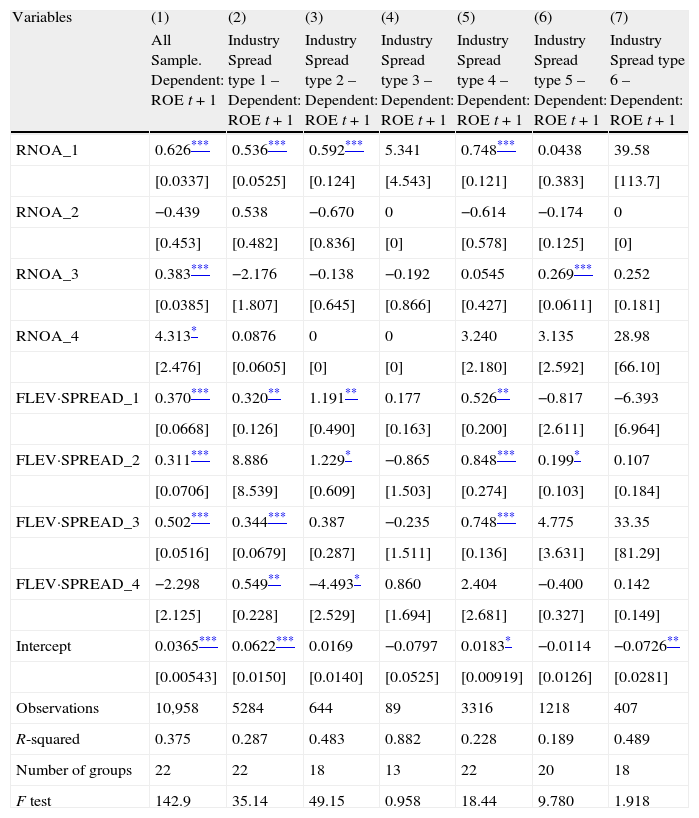
In Table 7 we have further disaggregated explanatory variables. Thus, in addition to the different types of industry spread and the four groups of RNOA, by signs of PM and ATO, we also disaggregate the second explanatory variable, according to the signs of FLEV and SPREAD.8 In this way, we can analyze the source of the signs and the values of the comprehensive variable FLEV·SPREAD in two dimensions: the relative position of firms and industries concerning profitability; and the sign of the two drivers behind the financial component of firm profitability, financial leverage and spread between operating and financing returns.
Disaggregating ROE levels by industry spread. Fama–MacBeth two-step procedure.
| Variables | (1) | (2) | (3) | (4) | (5) | (6) | (7) |
| All Sample. Dependent: ROE t+1 | Industry Spread type 1 – Dependent: ROE t+1 | Industry Spread type 2 – Dependent: ROE t+1 | Industry Spread type 3 – Dependent: ROE t+1 | Industry Spread type 4 – Dependent: ROE t+1 | Industry Spread type 5 – Dependent: ROE t+1 | Industry Spread type 6 – Dependent: ROE t+1 | |
| RNOA_1 | 0.626*** | 0.536*** | 0.592*** | 5.341 | 0.748*** | 0.0438 | 39.58 |
| [0.0337] | [0.0525] | [0.124] | [4.543] | [0.121] | [0.383] | [113.7] | |
| RNOA_2 | −0.439 | 0.538 | −0.670 | 0 | −0.614 | −0.174 | 0 |
| [0.453] | [0.482] | [0.836] | [0] | [0.578] | [0.125] | [0] | |
| RNOA_3 | 0.383*** | −2.176 | −0.138 | −0.192 | 0.0545 | 0.269*** | 0.252 |
| [0.0385] | [1.807] | [0.645] | [0.866] | [0.427] | [0.0611] | [0.181] | |
| RNOA_4 | 4.313* | 0.0876 | 0 | 0 | 3.240 | 3.135 | 28.98 |
| [2.476] | [0.0605] | [0] | [0] | [2.180] | [2.592] | [66.10] | |
| FLEV·SPREAD_1 | 0.370*** | 0.320** | 1.191** | 0.177 | 0.526** | −0.817 | −6.393 |
| [0.0668] | [0.126] | [0.490] | [0.163] | [0.200] | [2.611] | [6.964] | |
| FLEV·SPREAD_2 | 0.311*** | 8.886 | 1.229* | −0.865 | 0.848*** | 0.199* | 0.107 |
| [0.0706] | [8.539] | [0.609] | [1.503] | [0.274] | [0.103] | [0.184] | |
| FLEV·SPREAD_3 | 0.502*** | 0.344*** | 0.387 | −0.235 | 0.748*** | 4.775 | 33.35 |
| [0.0516] | [0.0679] | [0.287] | [1.511] | [0.136] | [3.631] | [81.29] | |
| FLEV·SPREAD_4 | −2.298 | 0.549** | −4.493* | 0.860 | 2.404 | −0.400 | 0.142 |
| [2.125] | [0.228] | [2.529] | [1.694] | [2.681] | [0.327] | [0.149] | |
| Intercept | 0.0365*** | 0.0622*** | 0.0169 | −0.0797 | 0.0183* | −0.0114 | −0.0726** |
| [0.00543] | [0.0150] | [0.0140] | [0.0525] | [0.00919] | [0.0126] | [0.0281] | |
| Observations | 10,958 | 5284 | 644 | 89 | 3316 | 1218 | 407 |
| R-squared | 0.375 | 0.287 | 0.483 | 0.882 | 0.228 | 0.189 | 0.489 |
| Number of groups | 22 | 22 | 18 | 13 | 22 | 20 | 18 |
| F test | 142.9 | 35.14 | 49.15 | 0.958 | 18.44 | 9.780 | 1.918 |
Standard errors in brackets.
Notes: ROE is the Return On Equity; RNOA is Return on Net Operating Assets (Operating Income/Net Operating Assets); FLEV is Financial Leverage (Net Financial Obligations/Book value of common equity); SPREAD is the difference between RNOA and Net Borrowing Cost (Net Financial Expense/Net Financial Obligations); RNOA_1 takes the value of RNOA if PM>0 and ATO>0, and 0 otherwise; RNOA_2 takes the value of RNOA if PM>0 and ATO<0, and 0 otherwise; RNOA_3 takes the value of RNOA if PM<0 and ATO>0, and 0 otherwise; RNOA_4 takes the value of RNOA if PM<0 and ATO<0, and 0 otherwise; FLEV·SPREAD_1 takes the value of FLEV·SPREAD if FLEV>0 and SPREAD >0, and 0 otherwise; FLEV·SPREAD_2 takes the value of FLEV·SPREAD if FLEV>0 and SPREAD <0, and 0 otherwise; FLEV·SPREAD_3 takes the value of FLEV·SPREAD if FLEV<0 and SPREAD >0, and 0 otherwise; FLEV·SPREAD_4 takes the value of FLEV·SPREAD if FLEV<0 and SPREAD <0, and 0 otherwise.
At first sight, the variable seems not very significant when both FLEV and SPREAD are negative. But analyzed in more detail, FLEV·SPREAD is a significant driver, at the 1% level, of the next-year ROE when both firms and industries show positive profitability, besides FLEV is negative and SPREAD is positive. For positive FLEV and negative SPREAD, the opposite is significant at the 1% level only when the industry's profitability is higher than the firm's profitability, suggesting that firm-specific structural deficiencies may be difficult to change in a year, in the line of McGahan and Porter (1997).
In general, our regression results show that FLEV contributes to the next-year positive ROE (col. 2, 3, and 5) when the spread is positive (FLESPREAD_1 and FLEV·SPREAD_3), and contributes to the next-year negative profitability (col. 6) when the spread is negative (FLEV·SPREAD_2), as shown in the portfolio analysis. Note that positive FLEV means indebtedness.
Another significant and interesting result is that even though the comprehensive coefficient for FLEV·SPREAD is not significant when both drivers are negative, after disaggregating the two components by sign, firms with profitability higher than the industry mean level show a contribution of this variable to the next-year ROE.
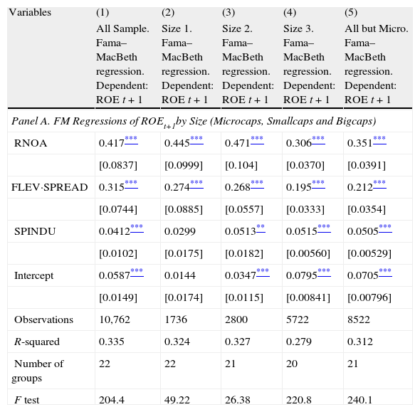
The role of industry spread in future profitability by firm sizeNow, we take size as a control variable in order to test if this factor may condition our results on profitability persistence and mean reversion in the presence of contextual information. We take into account Lewellen (2010), who states that empirical studies should report separate cross-sectional regressions for large stocks, not just pool all firms together. We follow this approach using the Fama and French (2008) criterion of classifying firms: microcaps are those smaller than the stock market capitalization 20th percentile each year in each country, small stocks are those between the stock market capitalization 20th and 50th percentiles each year in each country, and big stocks are those bigger than the stock market capitalization 50th percentile each year in each country.
Table 8 provides evidence on the importance of firm size to perform our tests on profitability persistence and mean reversion in the presence of industry-relative information more accurately. Specifically, this table shows the results obtained after having run regressions of Eq. (6) (Panel A) and Eq. (5) (Panel B), but considering different market values this time.
Regressions of ROE levels and changes by firm size.
| Variables | (1) | (2) | (3) | (4) | (5) |
| All Sample. Fama–MacBeth regression. Dependent: ROE t+1 | Size 1. Fama–MacBeth regression. Dependent: ROE t+1 | Size 2. Fama–MacBeth regression. Dependent: ROE t+1 | Size 3. Fama–MacBeth regression. Dependent: ROE t+1 | All but Micro. Fama–MacBeth regression. Dependent: ROE t+1 | |
| Panel A. FM Regressions of ROEt+1by Size (Microcaps, Smallcaps and Bigcaps) | |||||
| RNOA | 0.417*** | 0.445*** | 0.471*** | 0.306*** | 0.351*** |
| [0.0837] | [0.0999] | [0.104] | [0.0370] | [0.0391] | |
| FLEV·SPREAD | 0.315*** | 0.274*** | 0.268*** | 0.195*** | 0.212*** |
| [0.0744] | [0.0885] | [0.0557] | [0.0333] | [0.0354] | |
| SPINDU | 0.0412*** | 0.0299 | 0.0513** | 0.0515*** | 0.0505*** |
| [0.0102] | [0.0175] | [0.0182] | [0.00560] | [0.00529] | |
| Intercept | 0.0587*** | 0.0144 | 0.0347*** | 0.0795*** | 0.0705*** |
| [0.0149] | [0.0174] | [0.0115] | [0.00841] | [0.00796] | |
| Observations | 10,762 | 1736 | 2800 | 5722 | 8522 |
| R-squared | 0.335 | 0.324 | 0.327 | 0.279 | 0.312 |
| Number of groups | 22 | 22 | 21 | 20 | 21 |
| F test | 204.4 | 49.22 | 26.38 | 220.8 | 240.1 |
| Variables | (1) | (2) | (3) | (4) | (5) |
| All Sample. Fama–MacBeth regression. Change in ROE t+1 | Size 1. Fama–MacBeth regression. Change in ROE t+1 | Size 2. Fama–MacBeth regression. Change in ROE t+1 | Size 3. Fama–MacBeth regression. Change in ROE t+1 | All but Micro. Fama–MacBeth regression. Change in ROE t+1 | |
| Panel B. FM Regressions of ΔROEt+1by Size (Microcaps, Smallcaps and Bigcaps) | |||||
| ΔRNOA | −0.0286 | 0.109 | −0.0357 | −0.0221 | −0.0688** |
| [0.0486] | [0.206] | [0.0367] | [0.0977] | [0.0250] | |
| Δ(FLEV·SPREAD) | −0.0463 | 0.201 | −0.0651 | −0.0956 | −0.0953*** |
| [0.0619] | [0.284] | [0.0555] | [0.0630] | [0.0216] | |
| SPINDU | −0.0683*** | −0.0882*** | −0.0795*** | −0.0578*** | −0.0686*** |
| [0.00435] | [0.0108] | [0.00713] | [0.00553] | [0.00395] | |
| Intercept | −0.0130* | −0.0336*** | −0.0204** | −0.0136 | −0.0140* |
| [0.00692] | [0.00783] | [0.00779] | [0.00796] | [0.00706] | |
| Observations | 8306 | 1361 | 2148 | 4494 | 6642 |
| R-squared | 0.216 | 0.302 | 0.240 | 0.202 | 0.182 |
| Number of groups | 21 | 20 | 20 | 20 | 20 |
| F test | 134.4 | 23.17 | 46.57 | 70.65 | 108.4 |
Standard errors in brackets.
Notes: The table shows FM regressions for all stocks (all sample) and for Micro, Small, Big, and All but Micro stocks. Microcap stocks (Micro) are below the 20th percentile market cap at the end of the year, Small stocks are between the 20th and 50th percentiles, and Big stocks are above the median. All but Micro combines Small and Big stocks. This size classification follows Fama and French (2008) and Lewellen (2010). ROE is the Return On Equity; RNOA is Return on Net Operating Assets (Operating Income/Net Operating Assets); FLEV is Financial Leverage (Net Financial Obligations/Book value of common equity); SPREAD is the difference between RNOA and Net Borrowing Cost (Net Financial Expense/Net Financial Obligations); SPINDU is the difference between the firm's ROE and their Industry's average ROE, per country and year, deflacted by the standard deviation of industry ROE.
Previous results are generally confirmed, as a similar level of significance is maintained and most signs of coefficients are unchanged. In levels, both operating and financing factors are significant for any size, though the industry-relative factor has no significant effect in microcaps. The intercept is not significant either, indicating that there are no other relevant factors except for the firm-specific ones included in the model. If we focus on changes in profitability (Panel B), we find that industry-relative information is significant for any size of firms. Overall, after taking into account firm size, results confirm our previous findings. In addition, looking at the intercept values, we can interpret that the bigger the firms, the higher the stable profitability they can get. On the contrary, big firms do not show a stable pattern of change to mean values out of the industry-relative effect, and this pattern is lower than in the rest of firms.
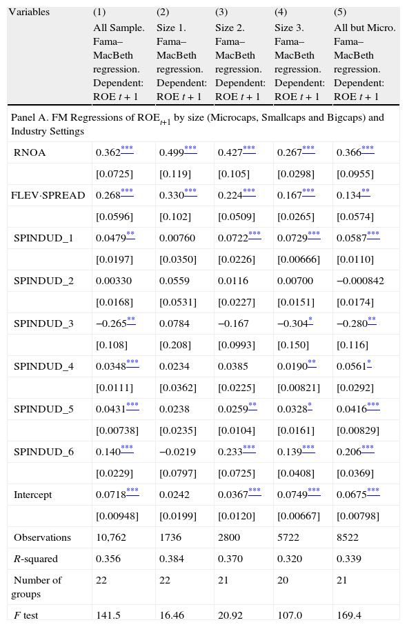
In Table 9, we have disaggregated the industry-relative variable into six variables, according to Fig. 1, in order to determine if previous results on the differences of profitability persistence and mean reverting for different industry-relative settings are homogeneous across different sizes of firms. In Panel A we confirm that the non-significant effect of the industry-relative variable on the next-year profitability of microcaps, observed in Table 8, is found across the six settings.
Regressions of ROE levels and changes by firm size in different industry settings.
| Variables | (1) | (2) | (3) | (4) | (5) |
| All Sample. Fama–MacBeth regression. Dependent: ROE t+1 | Size 1. Fama–MacBeth regression. Dependent: ROE t+1 | Size 2. Fama–MacBeth regression. Dependent: ROE t+1 | Size 3. Fama–MacBeth regression. Dependent: ROE t+1 | All but Micro. Fama–MacBeth regression. Dependent: ROE t+1 | |
| Panel A. FM Regressions of ROEt+1 by size (Microcaps, Smallcaps and Bigcaps) and Industry Settings | |||||
| RNOA | 0.362*** | 0.499*** | 0.427*** | 0.267*** | 0.366*** |
| [0.0725] | [0.119] | [0.105] | [0.0298] | [0.0955] | |
| FLEV·SPREAD | 0.268*** | 0.330*** | 0.224*** | 0.167*** | 0.134** |
| [0.0596] | [0.102] | [0.0509] | [0.0265] | [0.0574] | |
| SPINDUD_1 | 0.0479** | 0.00760 | 0.0722*** | 0.0729*** | 0.0587*** |
| [0.0197] | [0.0350] | [0.0226] | [0.00666] | [0.0110] | |
| SPINDUD_2 | 0.00330 | 0.0559 | 0.0116 | 0.00700 | −0.000842 |
| [0.0168] | [0.0531] | [0.0227] | [0.0151] | [0.0174] | |
| SPINDUD_3 | −0.265** | 0.0784 | −0.167 | −0.304* | −0.280** |
| [0.108] | [0.208] | [0.0993] | [0.150] | [0.116] | |
| SPINDUD_4 | 0.0348*** | 0.0234 | 0.0385 | 0.0190** | 0.0561* |
| [0.0111] | [0.0362] | [0.0225] | [0.00821] | [0.0292] | |
| SPINDUD_5 | 0.0431*** | 0.0238 | 0.0259** | 0.0328* | 0.0416*** |
| [0.00738] | [0.0235] | [0.0104] | [0.0161] | [0.00829] | |
| SPINDUD_6 | 0.140*** | −0.0219 | 0.233*** | 0.139*** | 0.206*** |
| [0.0229] | [0.0797] | [0.0725] | [0.0408] | [0.0369] | |
| Intercept | 0.0718*** | 0.0242 | 0.0367*** | 0.0749*** | 0.0675*** |
| [0.00948] | [0.0199] | [0.0120] | [0.00667] | [0.00798] | |
| Observations | 10,762 | 1736 | 2800 | 5722 | 8522 |
| R-squared | 0.356 | 0.384 | 0.370 | 0.320 | 0.339 |
| Number of groups | 22 | 22 | 21 | 20 | 21 |
| F test | 141.5 | 16.46 | 20.92 | 107.0 | 169.4 |
| Variables | (1) | (2) | (3) | (4) | (5) |
| All Sample. Fama–MacBeth regression. Change in ROE t+1 | Size 1. Fama–MacBeth regression. Change in ROE t+1 | Size 2. Fama–MacBeth regression. Change in ROE t+1 | Size 3. Fama–MacBeth regression. Change in ROE t+1 | All but Micro. Fama–MacBeth regression. Change in ROE t+1 | |
| Panel B. FM Regressions of ΔROEt+1 by Size (Microcaps, Smallcaps and Bigcaps) in industry settings | |||||
| ΔRNOA | 0.0130 | −0.0931* | −0.0264 | 0.121 | −0.0478** |
| [0.0696] | [0.0516] | [0.0381] | [0.215] | [0.0222] | |
| Δ(FLEV·SPREAD) | 0.0124 | −0.0865 | −0.0527 | −0.00267 | −0.0754*** |
| [0.101] | [0.0602] | [0.0568] | [0.133] | [0.0210] | |
| SPINDUD_1 | −0.0769*** | −0.0741** | −0.0619*** | −0.0458* | −0.0745*** |
| [0.00762] | [0.0299] | [0.0119] | [0.0224] | [0.00804] | |
| SPINDUD_2 | −0.0557*** | 0.0357 | 0.0139 | −0.0550*** | −0.0599*** |
| [0.0145] | [0.0529] | [0.0378] | [0.0142] | [0.0161] | |
| SPINDUD_3 | 0.149 | 0.528 | 0.0540 | 0.0649 | 0.00115 |
| [0.135] | [0.334] | [0.139] | [0.117] | [0.0879] | |
| SPINDUD_4 | 0.000115 | −0.0335 | −0.0153 | −0.0181 | 0.00283 |
| [0.00657] | [0.0348] | [0.0128] | [0.0182] | [0.00805] | |
| SPINDUD_5 | −0.0858*** | −0.0708*** | −0.105*** | −0.0867*** | −0.0975*** |
| [0.00840] | [0.0232] | [0.0131] | [0.0171] | [0.0103] | |
| SPINDUD_6 | −0.121*** | −0.175*** | −0.0331 | −0.151*** | −0.0928*** |
| [0.0184] | [0.0403] | [0.0477] | [0.0510] | [0.0252] | |
| Intercept | −0.00627 | −0.0255* | −0.0238*** | −0.0208 | −0.00841 |
| [0.00637] | [0.0146] | [0.00623] | [0.0164] | [0.00592] | |
| Observations | 8306 | 1361 | 2148 | 4494 | 6642 |
| R-squared | 0.268 | 0.403 | 0.307 | 0.267 | 0.230 |
| Number of groups | 21 | 20 | 20 | 20 | 20 |
| F test | 51.86 | 8.842 | 17.34 | 23.97 | 47.79 |
Standard errors in brackets.
Notes: The table shows FM regressions for all stocks (all sample) and for Micro, Small, Big, and All but Micro stocks. Microcap stocks (Micro) are below the 20th percentile market cap at the end of the year, Small stocks are between the 20th and 50th percentiles, and Big stocks are above the median. All but Micro combines Small and Big stocks. This size classification follows Fama and French (2008) and Lewellen (2010). ROE is the Return On Equity; RNOA is Return on Net Operating Assets (Operating Income/Net Operating Assets); FLEV is Financial Leverage (Net Financial Obligations/Book value of common equity); SPREAD is the difference between RNOA and Net Borrowing Cost (Net Financial Expense/Net Financial Obligations); SPINDUD_1 to SPINDUD_6 are the settings measured as the difference between the firm's ROE and their Industry's average ROE, deflacted by the standard deviation of the industry ROE, as explained in Fig. 1.
Once we have dropped microcaps, the industry-relative factor is significant at a higher level in the extremes: when both profitabilities are positive, if the firms’ profitability is higher than their industry's profitability; and when both profitabilities are negative, if the firms’ profitability is lower than their industry's profitability. In SPINDUD_2 (positive firm's profitability and negative industry's profitability), the industry-relative factor is not significant for any size of firms.
Furthermore, in settings SPINDUD_3 and SPINDUD_4 the industry relative factor seems to act only on big firms though in a less significant level. It suggests firms’ structural conditions harder to modify in big firms, making this type of firm more persistent in their negative profitability (SPINDUD_3) or in the negative effect of the difference respect to the industry (SPINDUD_4).
In Table 3, our results show that the industry-relative variable behaves as a reversion factor to offset the persistence of ROE in the autoregressive model, but it behaves as a persistence factor when RNOA and FLEV·SPREAD are the other explanatory variables of the model. In Table 8, we find that this industry-relative persistence factor is significant at the 1% level both for small and big firms, but for microcaps it does not contribute to the next-year ROE at all. In Table 9, our results show that the next-year ROE of microcaps is not explained by the industry-relative factor across the six industry-relative settings. Our results also show that for small and big firms the effect concentrates in the extreme industry-relative settings. The factor is not significant in SPINDUD_2 (positive firm's profitability and negative industry's profitability), and the negative effect on future profitability is only significant for big firms in SPINDUD_3 and SPINDUD_4.
As in Table 4, Panel B of Table 9 shows that the industry-relative factor explains the reversion in profitability changes better than RNOA or FLEV·SPREAD. But after disaggregating the industry-relative variable into six ones, according to the settings, we can see that the reversion effect appears only in the extremes (column 1) even though not homogeneously for the three sizes of firms. The reversion effect is similar in micro, small and big firms for SPINDUD_1 (firm's profitability higher than industry's profitability, being both positive) and for SPINDUD_5 (negative firm's profitability and positive firm's profitability). However, for SPINDUD_2 (positive firm's profitability and negative industry's profitability) only big firms show significant reversion, indicating that big firms are less able to keep their positive differences in profitability against the industry. On the other hand, microcaps are the group in which SPINDUD_6 is higher, suggesting their capability to revert negative profitability in a negative industry environment more effectively.
Concerning microcaps, our evidence indicates profitability less linked to the industry than in small or big firms. The current relative profitability of the firm with respect to the average profitability of the industry has no effect on the next-year profitability; however, the industry-relative factor has a more intense effect on changes in future profitability in the extremes, showing higher persistence of those differences in the extremes.
Robustness analysisFama and MacBeth's (1973) regressions produce standard errors robust to time effect, but the Fama–MacBeth variance estimation is too small in the presence of a firm effect (Petersen, 2009). If this is the case, standard errors would be understated (Thompson, 2011) and, as a consequence, too many t-statistics would be large in absolute values. Thus, residual dependence can result in misspecified test statistics. As Petersen (2009) and Gow, Ormazabal, and Taylor (2010) indicate, much of the empirical work in the accounting literature focuses exclusively on cross-sectional dependence and does not examine the issues which originated from the presence of both cross-sectional and time-series dependence.
To address these forms of dependence, a number of advances have been made. In this sense, recent research shows that two-way cluster-robust standard errors (CL-2) are robust to both time-series and cross-sectional correlation (Cameron, Gelbach, & Miller, 2011; Gow et al., 2010; Petersen, 2009; Thompson, 2011).
Petersen (2009) focuses on the financial literature and concludes that clustering standard errors by both firm and time appear unnecessary. However, Gow et al. (2010), highlight the fact that accounting variables exhibit greater dependence both over time and in cross-section, and find that, in a variety of accounting applications, two way cluster-robust standard errors are required for valid inferences. In untabulated results, we examine if our results can be attributable to biases induced by residual dependence. We repeat all regressions with CL-2, using the Stata routine written by Petersen (2009), and the results remain the same.
ConclusionFor an international sample (UK, Germany, France and Spain) over the 1981–2008 period, we document that disaggregating profitability into firm and industry information is useful in forecasting future levels and changes of ROE. We find that the impact of differences in profitability between each firm and its industry average value contributes to improve models on profitability prediction, whether for simple autoregressive models or for different levels of disaggregation of profitability drivers used as explanatory variables.
For the naive model, in the estimation of the next-year ROE considering only the information on the current-period ROE, the data on current profitability provide 60% of the information needed. However, if we consider the profitability status of the firm compared to that of the industry, we find that the coefficient of the current ROE variable is 0.63, while the relative status with respect to the industry leads to a reversal of approximately 1%. Furthermore, according to the signs and the relative positions of the firms’ profitability and the mean values of their industries’ profitability, we document a reversion pattern to reduce future ROE when the firm's profitability is higher than the industries’, though considerably lower for negative industries’ profitability; and stronger reversion patterns when the firms’ profitability is negative and lower than their industry's. We document similar differences in the weightings of the industry-relative factor when analyzing future changes in profitability instead of levels.
The intuition behind this result is straightforward. The industry structure conditions the conduct of member businesses. The structural characteristics of a certain industry may impede entry, support product differentiation, or otherwise limit rivalry among members. In this case, though competitors’ profitability levels differ due to individual features, their common context raises the average value of profitability. On the other hand, the lack of favorable structural conditions makes the average profitability decrease. As the variable industry spread is made by country, part of the differences in performance may rise because countries differ in their level of technological sophistication. Firms in the same country face similar macroeconomic conditions (capital cost, legal restrictions, political stability, NGP growth rate, …) which in turn affect their business and results.
Following Nissim and Penman (2001), we disaggregate current profitability into the relative contributions of operating activities and financing activities (first-level breakdown); but we also use the second-level breakdown into four profitability drivers: profit margin, asset turnover, leverage, and return spread. Unlike what was previously done, the use of sorts and disaggregation of drivers by signs allows us to keep firms in the sample regardless of the signs of the variables.
Thus, we document that the first level drivers of profitability, RNOA and FLEV·SPREAD, behave in a less linear pattern than ROE. Both the operating and the financing drivers of profitability are better inductors of the next-year ROE when the firm is performing well but falls behind the industry's benchmark. In this situation, an extra effort seems to be demanded to the individual firm. Similarly, when the industry's profitability is not a good benchmark for the firm (negative industry's profitability and positive firm's profitability), both current individual drivers are more weighting factors in future ROE. In this group, persistence of individual factors would help the firm to continue being profitable unlike the industry benchmark. In the most common setting, positive firm's profitability higher than its positive industry's profitability, both factors are significant but the next-year ROE seems to be partially explained by other persistent factors not specified in the model. Finally, in those models which include firms with negative profitability, the explanatory power of the current operating and financing drivers on the next-year ROE is lower, and the reversion factors are captured by the intercept.
After disaggregating RNOA into four different groups, according to the signs of its drivers, PM and ATO, we document that profit margin (either positive or negative) is not only the main driver of RNOA and ROE, but also of the next-year ROE. After doing the same type of disaggregation with the financing driver of profitability into FLEV and SPREAD, we document that leverage is just a multiplier of the main financing driver, the return spread. Another significant result not previously captured in the literature concerns both financing drivers negative. Even though the comprehensive coefficient for FLEV·SPREAD is not significant in this case, after disaggregating the two components by sign, firms with profitability higher than the industry mean level show a contribution of this variable to the next-year ROE. It is logical that those firms with financial investments higher than financial debts, obtaining financial returns higher than operating returns, make positive contributions to the next-year ROE. And it is reasonable that this contribution takes places only in profitable firms, as in other cases financial investments in non-financial firms would have been reduced until non-relevant levels.
Our expanded analysis by size finds microcaps less frequently linked to the industry benchmark of profitability, as the industry-relative factor has no effect on the next-year profitability in any setting, and profitability changes are more persistent in the extremes. Small and big firms behave similarly in the extremes, both by levels and by changes. More precisely, by levels we can observe that negative effects on big firms’ future profitability are stronger and generally more significant in non-extreme settings, while by changes, big firms seem to be less able to keep their non-extreme positive differences against industry. This suggests that the structural deficiencies are harder to be modified in big firms than in small firms, and that the negative industry benchmark is more influential in big firms than in small profitable firms.
As we connect two main strands of literature, we make different contributions to each of them. First, our work adds a new standpoint to the line of research that measures and quantifies the relative importance of contextual factors on the firm's performance, as proxied by profitability. Instead of analyzing co-movements of returns for different groups of firms, we analyze the persistence factor of profitability and the relative influence of the industry factors in it.
Second, instead of taking just the most commonly used indicator of performance, ROE; or the more recently used indicator, return of assets (Athanasoglou et al., 2008; Ball et al., 2009), our study starts from the seminal work of Nissim and Penman (2001) to disaggregate ROE into its first-level drivers: a more sophisticated version of return on assets (RNOA) to measure the operating part of profitability and a mixed component including financial leverage and return spreads to measure the financial part of profitability.
Third, to that more modern line significantly searching profitability persistence, our formulation of the industry factor contributes to fill the gap between the conclusions of Fama and French (2000) and those of Fairfield et al. (2009).
Fourth, for this profitability persistence line, our disaggregation of ROE into operating and financing drivers implies a contribution to previous studies as they focused only on ROE or ROA. Our study helps to determine the relative contribution of both operating and financing groups of activities on the profitability persistence. Furthermore, our study shows in which of both types of activities the industry-relative factor is playing a more relevant role.
Fifth, in order to identify non-lineal relations between the ROE drivers, resulting from Nissim and Penman (2001) disaggregation, our study uses sorts and breakdowns of first-level drivers by signs of second-level drivers, allowing us to make an in-depth analysis of the variable relations.
Finally, taking size as a control variable, we obtain revealing results on the profitability persistence of microcaps, small stocks, and big stocks, considering the industry-relative factor, and the operating and the financing activities of the companies.
Our results have important implications for investors, financial analysts, and business assessors as considering industry-relative information in straightforward methods they achieve higher comparability of firms and face lower information acquisition and lower processing costs. This is consistent with De Franco, Kothari, and Verdi (2011). findings that attribute more accurately forecasted earnings, at least in part, to a reduction in the forecast bias. Furthermore, our results are relevant for assessing the usefulness of disaggregated statements based on operating and financing activities, which supports the standard setters’ project (FASB, IASB) requiring that disaggregation.
Conflict of interestThe authors declare no conflict of interest.
The authors appreciate the helpful comments of the Editor, two anonymous reviewers of SAR, Stephen Penman, Aljosa Valentincic, and the participants at the EAA Annual Congress in Ljubliana. Also, we are grateful for comments received to previous versions of the paper from participants at the Workshop on Empirical Research in Financial Accounting in Sevilla, and the EAA Annual Congress in Rome. This research is funded by the ECO2011-29144-C03-01 research project of the Spanish Ministry of Science and Innovation, and the ULE2012-1 research project of the University of Leon.
A recent work of Li et al. (2011) documents lower future ROE in more competitive industries.
Note that the industry relative factor is constructed by country; hence, part of the industry variable captures country trends.
Fama and French (2000) forecast the following change in profitability with a model of partial adjustment that employs two pieces of information: (1) the more recent change in profitability – from t−1 to t –; and (2) the deviation of profitability from its expected value. They use a two-step approach because the expected value of profitability needs to be estimated previously by applying some assumptions. However, as an unobservable figure, expected profitability is a noisy variable subject to some restrictions imposed by initial assumptions and by omitted variable bias.
We construct our variables starting from Worldscope data, while Nissim and Penman use Compustat, therefore some slight differences could be found.
The Fama–French (FF) classification has been highly influential, being widely used in many academic studies on finance and accounting. The composition of the industries is described in detail in Kenneth French's website: http://mba.tuck.dartmouth.edu/pages/faculty/ken.french/.
Our approach follows that of Fama and French (2008) but we construct sorts on our proposed industry spread variables. To avoid the potential problem of general results dominated by tiny firms (microcaps) when using equal-weight decile portfolios, we separately perform our regressions on microcaps, small, and big firms given in role of industry spread in future profitability by firm size section.
As explained in Portfolio approach section, each of these six continuous variables takes the value of SPINDU when the signs are the selected for the group and 0 otherwise. Thus, SPINDU_1 takes the value of SPINDU when firm's ROE≥Industry ROE, being both positive (vid. Fig. 1).
Each of these variables, FLEV SPREAD_1 to FLEV SPREAD_4, is a continuous variable that takes the value of the variable FLEV SPREAD when the signs are the selected for the group and 0 otherwise.

www.publicationethics.org.