
Viral and infectious diseases such as COVID-19 continue to pose a significant public health threat. In order to create an early warning system for new pandemics or emerging versions of the virus, it is imperative to study its epidemiology. In this study, we created a geospatial model to predict the weekly contagion and lethality rates of COVID-19 in Ireland.
MethodsMore than forty parameters including atmospheric pollutants, metrological variables, sociodemographic factors, and lockdown phases were introduced as input variables to the model. The significant parameters in predicting the number of new cases and the death toll were identified. QGIS software was employed to process input data, and a principal component regression (PCR) model was developed using the statistical add-on XLSTAT.
Results and conclusionsThe developed models were able to predict more than half of the variations in contagion and lethality rates. This indicates that the proposed model can serve to help prediction systems for the identification of future high-risk conditions. Nevertheless, there are additional parameters that could be included in future models, such as the number of deaths in care homes, the percentage of contagion and mortality among health workers, and the degree of compliance with social distancing.
Las enfermedades virales e infecciosas como la COVID-19 continúan representando una importante amenaza para la salud pública. Para crear un sistema de alerta temprana para nuevas pandemias o versiones emergentes del virus es imperativo estudiar su epidemiología. En este estudio creamos un modelo geoespacial para predecir las tasas semanales de contagio y de letalidad de la COVID-19 en Irlanda.
MétodosSe introdujeron más de cuarenta parámetros, incluidos contaminantes atmosféricos, variables meteorológicas, factores sociodemográficos y fases de confinamiento, como variables de entrada al modelo. Se identificaron los parámetros significativos para predecir el número de casos nuevos y el número de muertes. Se empleó el software QGIS para procesar los datos de entrada y se desarrolló un modelo de regresión de componentes principales (PCR) utilizando el complemento estadístico XLSTAT.
Resultados y conclusionesLos modelos desarrollados fueron capaces de predecir más de la mitad de las variaciones en las tasas de contagio y de letalidad. Esto indica que el modelo propuesto puede servir para ayudar a los sistemas de predicción en la identificación de condiciones futuras de alto riesgo. No obstante, existen parámetros adicionales que podrían incluirse en futuros modelos, como el número de muertes en residencias, el porcentaje de contagio y de mortalidad entre el personal sanitario y el grado de compatibilidad con la distancia social.
The ongoing global COVID-19 pandemic caused by the spread of the SARS-CoV-2 virus had a catastrophic effect on human health and global economies since 2019. In terms of risk groups, the elderly and those with underlying medical conditions were disproportionally affected by the virus, with a correspondingly higher number of fatalities.1 Generally, people over 70 years of age and those with pre-existing diseases, such as arterial hypertension, heart problems, diabetes, chronic respiratory diseases, cancer, and immunosuppressed patients were more likely to develop severe forms of the disease.2
Although considerable research has been devoted to studying the effect of the virus on different groups of people, rather less attention has been paid to the effect of environmental factors (i.e. atmospheric pollution and metrological parameters) on the transmission and infection rates. As an example of the effect of atmospheric parameters, fine powders and aerosols can provide the possibility for viruses to attach themselves to fine dust present in the air and thus be transported by the wind for large distances or remain suspended in the air.3 A study done by Conticini et al. showed that the high air pollution loading could be a co-factor causing the high fatality rate due to the COVID-19 infection.4 Other recent studies5–7 highlighted the links between prior exposure to air pollution and COVID-19. It is important to note that while many variables that contribute to the transmission and severity of COVID-19, such as age, temperature, and wind speed, are beyond the control of primary care practitioners, it is still crucial for them to have a comprehensive understanding of the epidemiological aspects of the disease. This knowledge can help them better inform their patients about the risk factors associated with COVID-19 and how to mitigate them. Regarding the association between air pollution and COVID-19, previous studies (mentioned above) have shown that exposure to air pollution can worsen the health effects of COVID-19 by suppressing immunity and increasing the risk of death. However, there is still limited research on the relationship between air pollution and COVID-19 infection and mortality rates. Therefore, it is essential to consider the effect of atmospheric pollution, including PM10, PM2.5, O3, SO2, and NO2, as an additional co-factor that can increase the lethality of COVID-19 or similar viral infections.8
By taking into account the impact of atmospheric pollution on COVID-19, physicians and medical practitioners can better understand how environmental factors can contribute to the severity of the disease. This knowledge can help them provide more comprehensive care to their patients by providing advice on how to minimize exposure to air pollution and other environmental factors that may exacerbate their symptoms. Ultimately, this can lead to better outcomes for patients and a more effective response to the ongoing COVID-19 pandemic should be considered as an additional co-factor for increasing the level of COVID-19 or similar viral infections’ lethality.
Among the atmospheric factors that have been studied in the following research,4,7,9 the pollutants PM2.5, ozone (O3), sulphur dioxide (SO2), and to a lesser extent PM10 showed a positive correlation with virus transmission. Another study conducted in Saudi Arabia10 showed that the number of COVID-19 positive cases increases when the atmospheric temperature, air humidity or average wind speed decreases. Furthermore,11 showed a positive association between daily new cases of COVID-19 with low temperatures. In that research,11 relative and absolute humidity was also found to have a clear association with daily new cases of COVID-19. It was concluded that COVID-19 pandemic transmission favours dry and cool environmental conditions, as well as polluted air. For those reasons, the virus might spread more easily in unfiltered air-conditioned indoor environments.9
Given that COVID-19 attacks the respiratory system, environmental factors that impact respiratory health (such as exposure to radon) may leave an individual more disposed to infection. The adverse effect of radon on the lungs existed long before the arrival of COVID-19.12,13 There are no scientific reports or technical evaluations between coronavirus and radon yet; however as both affect the respiratory system, the occurrence of elevated levels of radon will expose lungs to an environmental exposure which has a measureable negative health effect.14 For example, in the Lombardy province of Italy, one of the regions most affected by COVID-19, there are approximately 200,000 homes at enhanced risk of radon (4.1% of the total).15,16
Value of the dataThe research methodology presented here can be effectively utilized for modelling COVID-19 contagion and lethality in other countries. The prediction models prepared in this study are valid for initial variants of SARS-CoV-2. However, the same methodology can be adopted for future variants of the virus. It is also possible to update the models by including additional input parameters and running the models through longer periods. The results of this project may be extended and used also for modelling other viral infections like Influenza, and Ebola.
ObjectiveThis proof of concept study aims to gain a better understanding of (a) environmental exposures, which may lead to increased severe acute respiratory syndrome infection rates, (b) the impact of gender-specific lifestyle, health condition and vulnerability by age and sex, and also (c) the impact of setting lockdown and physical distancing. In this paper, the spatial association between socio-demographic composition, atmospheric pollution, weather data and lockdown phases are investigated by developing a comprehensive principal components regression (PCR) model that predicts the weekly COVID-19 deaths and cases. Such a prediction model can serve as a toolkit to support decision-making on local, regional, national, or international levels. Our prediction model can improve public health, through focused restrictions for the most at-risk locations and groups. It may as well be used by governments and health agencies to make informed decisions for planning and mitigation of future outbreaks of highly infectious and acute respiratory diseases.
Materials and methodsData descriptionBackground information on COVID-19 pandemic in IrelandThe COVID-19 pandemic reached the Republic of Ireland on 29 February 2020, and within three weeks, cases had been confirmed in all counties. The first wave of the virus was between February – May 2020 adding that the peak of daily new cases and confirmed death was reported in mid-April 2020. Later the National Public Health Emergency Team reported that the lockdown and other measures had decreased the growth rate of the pandemic. Due to a significant fall in the contagion and lethality rate, the Irish government began to ease COVID-19 restrictions in early May 2020. The easing of restrictions continued until August 2020. The second wave of virus spread combined with a significant increase of COVID-19 cases in the three counties (i.e. Kildare, Laois, and Offaly) pushed towards a set of new restrictive measures in early August. In October 2020, Ireland imposed its highest level of national restrictions as part of a lockdown that will last six weeks. By the date of writing this paper (January–February 2021), Ireland was passing the second week of the COVID-19 pandemic. But as can be understood from the daily statistical data published by the Government of Ireland, it seems that the full lockdown has beaten the second COVID-19 wave in Ireland.17
As shown in Figure S-1 (Appendix A), for the period of 03 April to 30 October 2020, Counties Meath, Cork, and Laois have the highest total weekly rates of new cases among all Irish counties. Counties Laois, Limerick, and Wexford also have the highest total weekly death rates. The number of cases in Ireland translates to a rate of around 1430 cases per 100,000 population. In terms of deaths from the virus, Ireland has recorded 41.23 deaths per 100,000 population, which was the tenth highest in the EEA as of November 22, 2020. Like other Western European countries, high COVID-19 morbidity and mortality (about 20% of total death) were observed among residents in long-term care facilities.18
Lockdown phases in IrelandOn 12 March 2020, the Irish government closed all schools, colleges, childcare facilities, and cultural institutions, and advised cancelling large gatherings. On 24 March, almost all businesses, venues, facilities, and amenities were shut; but gatherings of up to four were allowed. Three days later on 27 March, the government imposed a stay-at-home order, banning all non-essential travel and contact with people outside one's home including family and partners. The elderly and those with certain health conditions were told to cocoon. People were advised to keep their distance in public. A roadmap to easing restrictions in Ireland that includes five stages was adopted by the government to be implemented by the beginning of 18 May 2020. On 18 August, the Government of Ireland announced six new measures because of the growing number of confirmed cases, which remained in place until 15 September. On 15 September, the Government of Ireland announced a medium-term plan for living with COVID-19 that includes five levels of restrictions, with the entire country at Level 2 and specific restrictions in Dublin including the postponement of the reopening of pubs not serving food.19
Input dataThe input data can be classified into four main categories:
- 1)
Atmospheric pollution: PM10, PM2.5, O3, SO2 and NO2 recorded by 84 monitoring stations distributed over the state (see Figure S-2 (Appendix A)) that are managed by the Environmental Protection Agency of Ireland (EPA-www.epa.ie) as well as annual averages of indoor radon activity provided by EPA.
- 2)
Meteorological elements: precipitation amount, air temperature, wet bulb air temperature, dew point air temperature, vapour pressure, relative humidity, mean sea level pressure, mean hourly wind speed, predominant hourly wind direction and the sunshine duration recorded by 25 monitoring stations (see Figure S-2 (Appendix A)) on a minute-by-minute basis. The metrological data was provided by Met Éireann (www.met.ie), Met Éireann, the Irish National Meteorological Service based in Dublin.
- 3)
Sociodemographic information provided as a result of the report of the 2016 census of Ireland (www.cso.ie) which includes data on self-perceived health status in ordinal category (very bad to very good), population, population density, and distribution of sex and age profile.
- 4)
Lockdown phases (5 stages) set by the Irish government (www.gov.ie).
The input data were processed in the open-source QGIS Desktop 3.16.2 software (Hannover) (www.qgis.org). First, the geo-referenced point layers showing the location of weather and air pollution monitoring stations in Ireland were created (Figure S-2 (Appendix A)) and the shapefile of the County borders of Ireland was added. Then, the atmospheric pollutants and the data on metrological parameters were downloaded, the weekly averages and standard deviations were calculated and the mean values were assigned to the database of each point. Using the “Join attributes by location tool” the weekly averages of the studied parameters were calculated for the points located within the borders of each county. The weekly statistics of new COVID-19 cases and deaths reported by the Health Surveillance Protection Centre (www.data.gov.ie) were also downloaded for all Irish counties for the period of 03 April to 30 October 2020. These data were assigned to the database of the Counties’ shapefile. Up to this step, the database of the county shapefile contains weekly averages of atmospheric and metrological parameters as well as the weekly sum of new cases and deaths. In the next step, the sociodemographic data of each county were added to the database of the county shapefile. The Sociodemographic data used in this study includes the breakdown of the population estimates (percent of the total population) by region, sex, and age as well as health status. Finally, the level of lockdown phases obtained from reports of the Irish government were assigned to the same database. The tabular file was saved as a CSV file which contained information on 41 variables for each of the 26 Irish counties. It is noteworthy that a high degree of skewness was observed in the weekly COVID-19 contagion and death rates hence these two data were log-normally transferred to reduce the skewness before the model setting began.
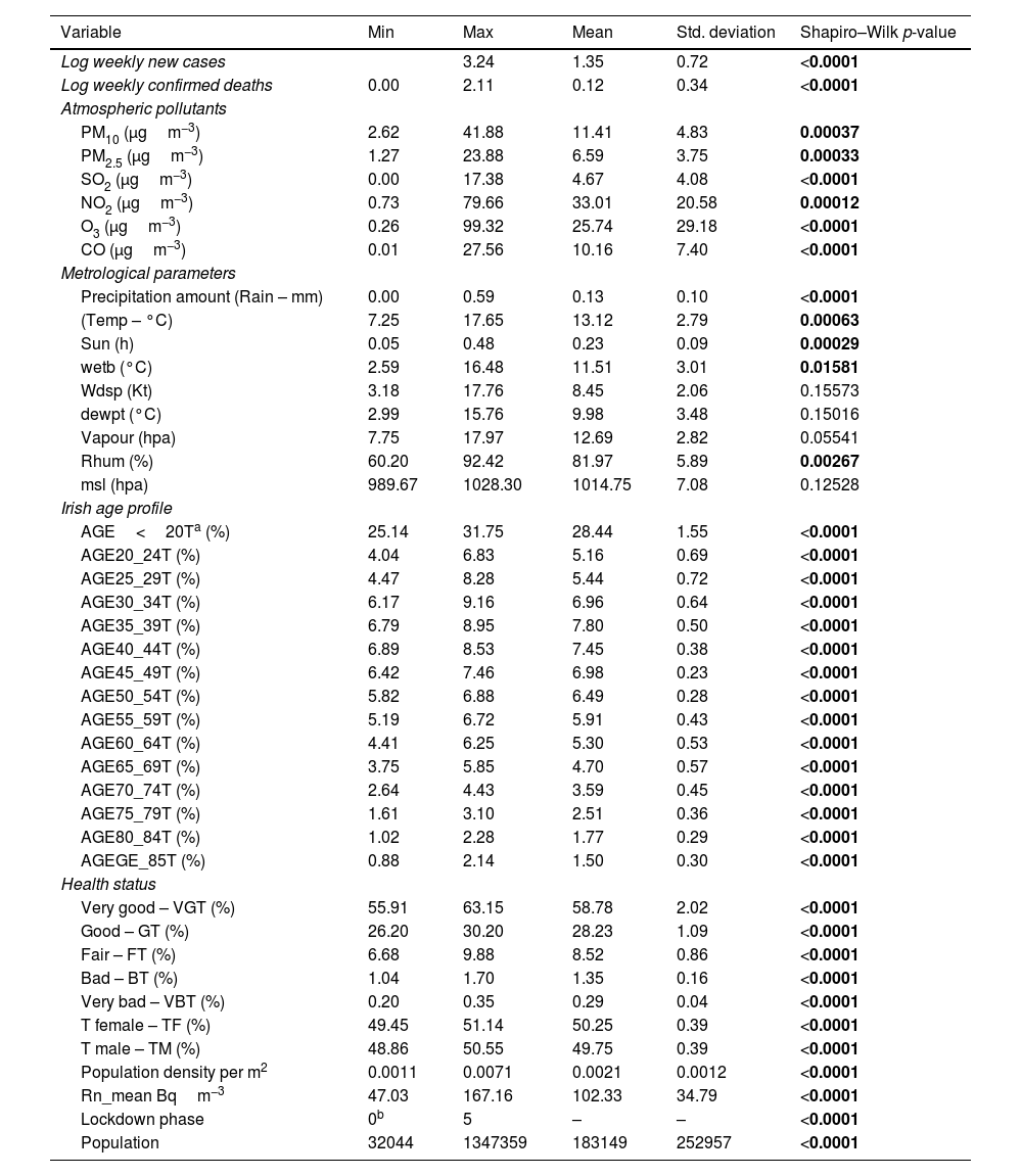
Model settingThe first step to setting up a prediction model is to define the response variables/s and specify the explanatory parameters. The weekly sum of COVID-19 cases and deaths were considered as response variables and the 41 input parameters were defined as predictors. Table 1 shows the input parameters and a summary of their statistics. In the next step, the spatial association between socio-demographic composition, atmospheric pollution, weather data, and COVID-19 deaths and cases were evaluated by developing a comprehensive principal components regression (PCR) model. The table presents a comprehensive summary of various statistical measures across different variables, providing insights into a wide range of factors. In the context of the COVID-19 pandemic, the data show that the logarithmically transformed weekly new cases range from 0.00 to 3.24, with a mean of 1.35 and a standard deviation of 0.72. Similarly, for logarithmically transformed weekly confirmed deaths, the range is 0.00 to 2.11, with a mean of 0.12 and a standard deviation of 0.34. These statistics highlight significant variability in case and death numbers. Additionally, the low p-values from the Shapiro–Wilk tests (<0.0001) suggest that both variables do not follow a normal distribution.
Summary of the statistics and normality test of response and predictor variables.
| Variable | Min | Max | Mean | Std. deviation | Shapiro–Wilk p-value |
|---|---|---|---|---|---|
| Log weekly new cases | 3.24 | 1.35 | 0.72 | <0.0001 | |
| Log weekly confirmed deaths | 0.00 | 2.11 | 0.12 | 0.34 | <0.0001 |
| Atmospheric pollutants | |||||
| PM10 (μgm−3) | 2.62 | 41.88 | 11.41 | 4.83 | 0.00037 |
| PM2.5 (μgm−3) | 1.27 | 23.88 | 6.59 | 3.75 | 0.00033 |
| SO2 (μgm−3) | 0.00 | 17.38 | 4.67 | 4.08 | <0.0001 |
| NO2 (μgm−3) | 0.73 | 79.66 | 33.01 | 20.58 | 0.00012 |
| O3 (μgm−3) | 0.26 | 99.32 | 25.74 | 29.18 | <0.0001 |
| CO (μgm−3) | 0.01 | 27.56 | 10.16 | 7.40 | <0.0001 |
| Metrological parameters | |||||
| Precipitation amount (Rain – mm) | 0.00 | 0.59 | 0.13 | 0.10 | <0.0001 |
| (Temp – °C) | 7.25 | 17.65 | 13.12 | 2.79 | 0.00063 |
| Sun (h) | 0.05 | 0.48 | 0.23 | 0.09 | 0.00029 |
| wetb (°C) | 2.59 | 16.48 | 11.51 | 3.01 | 0.01581 |
| Wdsp (Kt) | 3.18 | 17.76 | 8.45 | 2.06 | 0.15573 |
| dewpt (°C) | 2.99 | 15.76 | 9.98 | 3.48 | 0.15016 |
| Vapour (hpa) | 7.75 | 17.97 | 12.69 | 2.82 | 0.05541 |
| Rhum (%) | 60.20 | 92.42 | 81.97 | 5.89 | 0.00267 |
| msl (hpa) | 989.67 | 1028.30 | 1014.75 | 7.08 | 0.12528 |
| Irish age profile | |||||
| AGE<20Ta (%) | 25.14 | 31.75 | 28.44 | 1.55 | <0.0001 |
| AGE20_24T (%) | 4.04 | 6.83 | 5.16 | 0.69 | <0.0001 |
| AGE25_29T (%) | 4.47 | 8.28 | 5.44 | 0.72 | <0.0001 |
| AGE30_34T (%) | 6.17 | 9.16 | 6.96 | 0.64 | <0.0001 |
| AGE35_39T (%) | 6.79 | 8.95 | 7.80 | 0.50 | <0.0001 |
| AGE40_44T (%) | 6.89 | 8.53 | 7.45 | 0.38 | <0.0001 |
| AGE45_49T (%) | 6.42 | 7.46 | 6.98 | 0.23 | <0.0001 |
| AGE50_54T (%) | 5.82 | 6.88 | 6.49 | 0.28 | <0.0001 |
| AGE55_59T (%) | 5.19 | 6.72 | 5.91 | 0.43 | <0.0001 |
| AGE60_64T (%) | 4.41 | 6.25 | 5.30 | 0.53 | <0.0001 |
| AGE65_69T (%) | 3.75 | 5.85 | 4.70 | 0.57 | <0.0001 |
| AGE70_74T (%) | 2.64 | 4.43 | 3.59 | 0.45 | <0.0001 |
| AGE75_79T (%) | 1.61 | 3.10 | 2.51 | 0.36 | <0.0001 |
| AGE80_84T (%) | 1.02 | 2.28 | 1.77 | 0.29 | <0.0001 |
| AGEGE_85T (%) | 0.88 | 2.14 | 1.50 | 0.30 | <0.0001 |
| Health status | |||||
| Very good – VGT (%) | 55.91 | 63.15 | 58.78 | 2.02 | <0.0001 |
| Good – GT (%) | 26.20 | 30.20 | 28.23 | 1.09 | <0.0001 |
| Fair – FT (%) | 6.68 | 9.88 | 8.52 | 0.86 | <0.0001 |
| Bad – BT (%) | 1.04 | 1.70 | 1.35 | 0.16 | <0.0001 |
| Very bad – VBT (%) | 0.20 | 0.35 | 0.29 | 0.04 | <0.0001 |
| T female – TF (%) | 49.45 | 51.14 | 50.25 | 0.39 | <0.0001 |
| T male – TM (%) | 48.86 | 50.55 | 49.75 | 0.39 | <0.0001 |
| Population density per m2 | 0.0011 | 0.0071 | 0.0021 | 0.0012 | <0.0001 |
| Rn_mean Bqm−3 | 47.03 | 167.16 | 102.33 | 34.79 | <0.0001 |
| Lockdown phase | 0b | 5 | – | – | <0.0001 |
| Population | 32044 | 1347359 | 183149 | 252957 | <0.0001 |
In the second section, various environmental and demographic variables are explored. For instance, atmospheric pollutants like PM10 have a mean value of 11.41μgm−3 and a standard deviation of 4.83, while the precipitation amount (Rain-mm) has a mean of 0.13mm and a standard deviation of 0.10. In terms of age profiles, the percentage of the population in the 25–29 age group is around 5.44%, with low variability (standard deviation of 0.72). Furthermore, health statuses are represented, where around 58.78% of the population reported being in “Very Good” health, with a standard deviation of 2.02. These statistics, along with low p-values across various variables, provide valuable insights into environmental, demographic, and health-related factors, facilitating further analysis and exploration of potential relationships among these variables.
Principal components regression (PCR) which was introduced and clearly explained by Jolliffe and Cadima20 is a regression method that includes three main operations. The first step is to run a principal components analysis (PCA) on the table of the explanatory variables. Then running an ordinary least squares (OLS) regression also called linear regression on the selected components and finally compute the parameters of the model that correspond to the input variables. PCA and PCR are among the highly recommended techniques for improving regression models.21 The regression analysis (PCR) of these principal components (PCs) as independent variables will yield an appropriate estimation of the response parameter. As PCR is built on PCA, a great advantage of PCR regression over classical regression is the available charts that describe the data structure. Besides, PCR has several other advantages; it solves the dimensionality among the datasets and it is robust against collinearity between predictor variables.22 The PCR method employed in this study uses the first principal components that have a cumulative proportion of total variance of at least 95% to simulate daily new cases and confirmed deaths of COVID-19 as the dependent variables of the model. The equation used is as follows:

Y1=COVID-19 weekly new cases estimation and Y2=COVID-19 weekly deaths estimation; Z=Principal components; a=constant; b=regression coefficient of Z with respect to Y.
The main purpose of applying PCA was to identify the socio-demographic composition, atmospheric pollution, and weather data (predictors) that are significantly correlated with the contagion and lethality rates of COVID-19. In particular, PCA accounts for interactions between all predictors and attributes these interactions to PCs. The PCs that explained most of the variance were included in the regression model (PCR). XLSTAT23 was used for statistical analysis. Although XLSTAT is provided as an add-on for Microsoft Excel, it is an independent software that can be used in an Excel environment to perform various statistical analyses in our case; principal component analysis, calculation of the correlation matrix, estimation of Cook's distance, determination of Eigenvalues, and interpretation of the results.
Model validationStandard deviation (σ) and standard error (SE), as well as the size of the root mean square error (RMSE), mean square error (MSE), mean absolute error (MAE), and the cross-validation between the observed and the predicted values of new cases and deaths of COVID-19, were used to evaluate the goodness of the PCR model.24,25 The σ, SD, SE, RMSE, and MSE are defined as follows:
where n=the number of data points, Yi=observed values, Ÿ=mean and Ŷi=predicted values.ResultsPrincipal component analysis (PCA)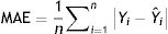

Table S-1 (Appendix B) shows the eigenvalues calculated based on the principal component analysis (PCA). In the PCA, the eigenvectors (principal components) determine the directions of the new feature space while the eigenvalues determine their magnitude which reflects the quality of the projection from the N-dimensional initial database (N=39 in this example) to a lower number of dimensions.20 According to this table, the first eigenvalue equals 12.66 and represents 30.87% of the total variability. This means that if the data are represented on only one axis, it would be possible to see 30.87% of its total variability.
Each eigenvalue corresponds to a factor and each factor represents one dimension. A factor is a linear combination of the initial variables, and all the factors are uncorrelated (R2=0). The eigenvalues and the corresponding factors are sorted by descending order of how much of the initial variability they represent (converted to %) (see Figure S-3 (Appendix B)).
Ideally, the first sets of eigenvalues will correspond to a high % of the variance, ensuring that the results based on the first two or three factors are a good-quality projection of the initial multi-dimensional database. In this example, a good result was found since the first eleven factors allow us to represent 90.86% of the initial variability of the data. However, attention should be paid when interpreting the factors because some information might be hidden in the next factors. On the other hand, one can notice that although there were initially 41 variables, the number of considered factors is 39. This is due to the elimination percent of two variables, which are negatively correlated (R2=−1). The number of “useful” dimensions was automatically detected by XLSTAT.
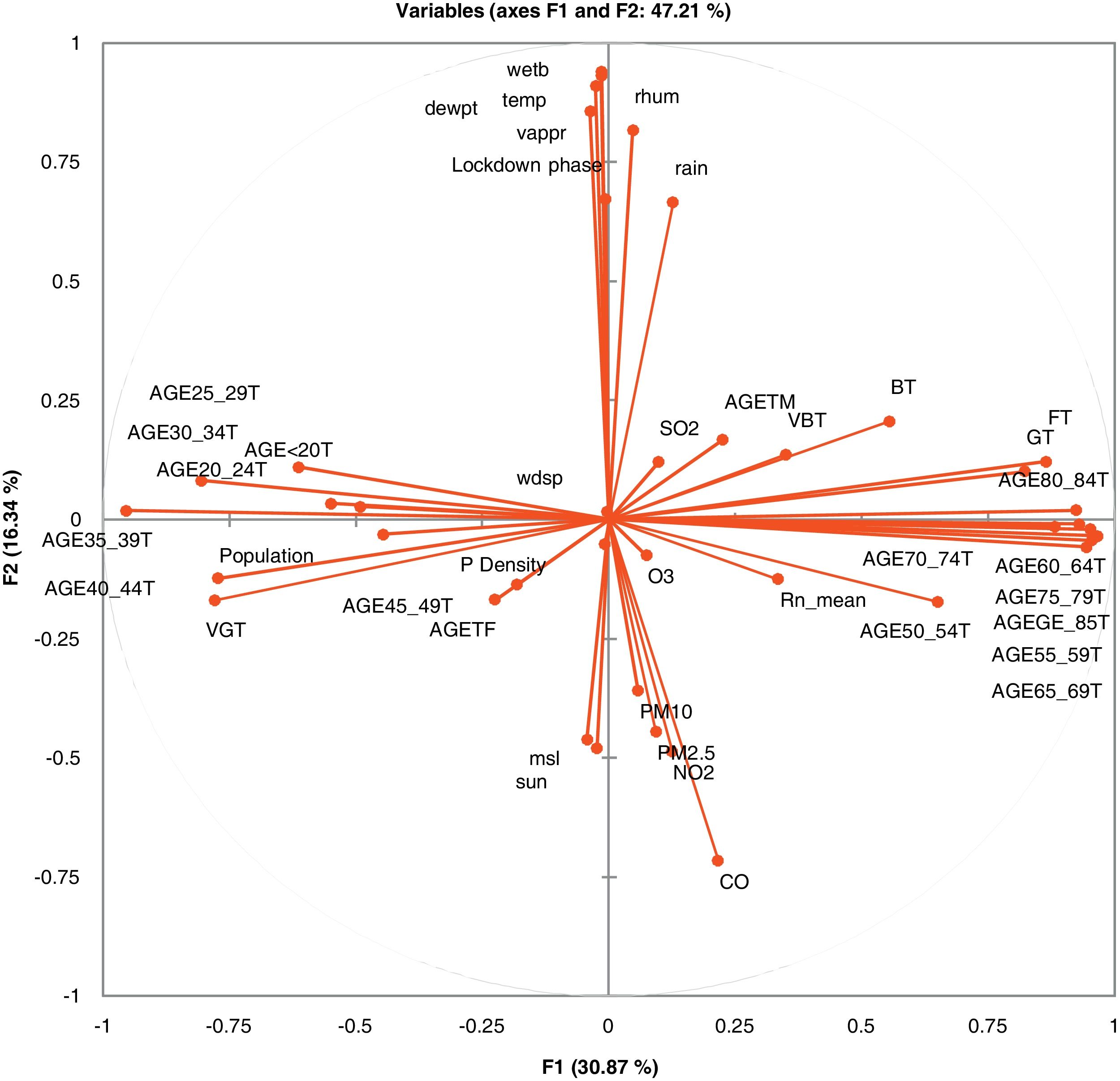
In Fig. 1, the correlation circle shows a projection of the initial variables in the factors space. When two variables are far from the centre, then, if they are close to each other, they are significantly positively correlated (R2 close to 1); if they are orthogonal, they are not correlated (R2 close to 0) and if they are on the opposite side of the centre, then they are significantly negatively correlated.

When the variables are close to the centre, some information is carried on other axes and because of that, any interpretation might be hazardous. For example, it might be tempting to interpret a correlation between the variables CO and mean radon although there is none. This can be confirmed either by cross-checking the correlation matrix or by looking at the correlation circle on axes F1 and F3. The correlation circle is useful in interpreting the meaning of the axes. In this example, the horizontal axis is linked with age categories and the vertical axis with weather data. These trends will help interpret the next parameter to confirm that a variable is well-linked with an axis.
Principal components regression (PCR)Table S-2 (Appendix C) shows the goodness of fit coefficients of models for the prediction of weekly new cases and confirmed deaths of COVID-19. The R2 (coefficient of determination) indicates the percent of the variability of the dependent variable which is explained by the explanatory variables. R2 values greater than 0.5 are good. The closer to 1 the R2 is, the better the fit. In the case of this study, 53% and 54% of the variability of the contagion and lethality are explained by the predictors. The remainder of the variability is due to effects that have not been included in this analysis (variables like the degree of actual social distancing, blood groups, etc.).
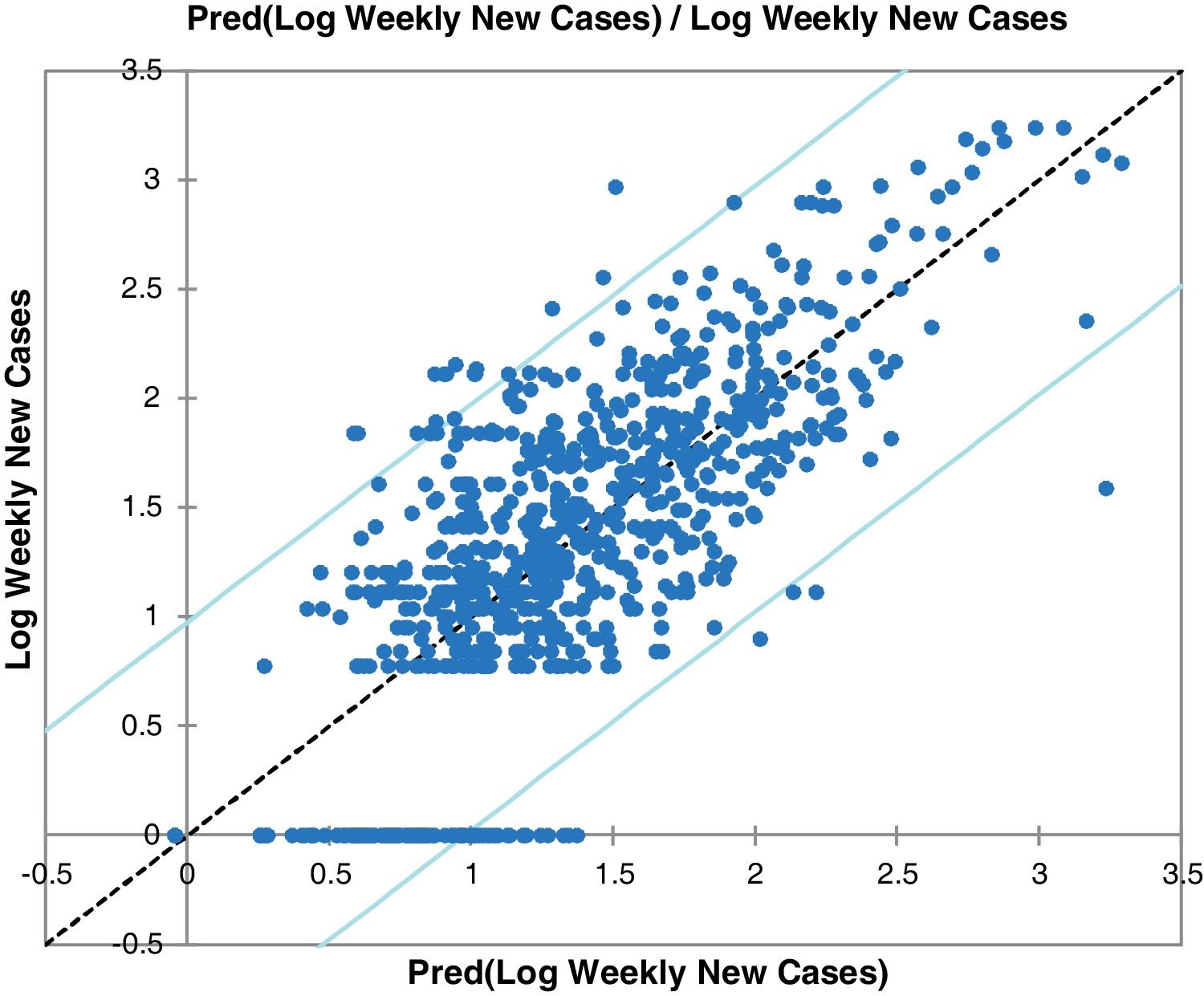
Fig. 2 and Figure S-4 (Appendix C) show the correlations between predicted and observed values of COVID-19 weekly new cases and confirmed deaths. The 95% confidence level intervals are also shown in the charts of these figures. The values out of the space between confidence levels are potential outliers or might suggest that the normality assumption is wrong.

It is also important to examine the results of the analysis of variance presented in Table S-3 (Appendix C). The results allow us to determine whether or not the explanatory variables bring significant information (null hypothesis) to the model. In other words, it's a way of asking whether it is valid to use the mean to describe the whole population, or whether the information brought by the explanatory variables is of value or not. Fisher's F test is used for this purpose. Given the fact that the probability corresponding to the F value is lower than 0.0001, it means that we would be taking a lower than 0.01% risk in assuming that the null hypothesis is wrong. Therefore, it can be concluded that the 41 variables bring a significant amount of information to the models for the prediction of contagion and lethality rates.
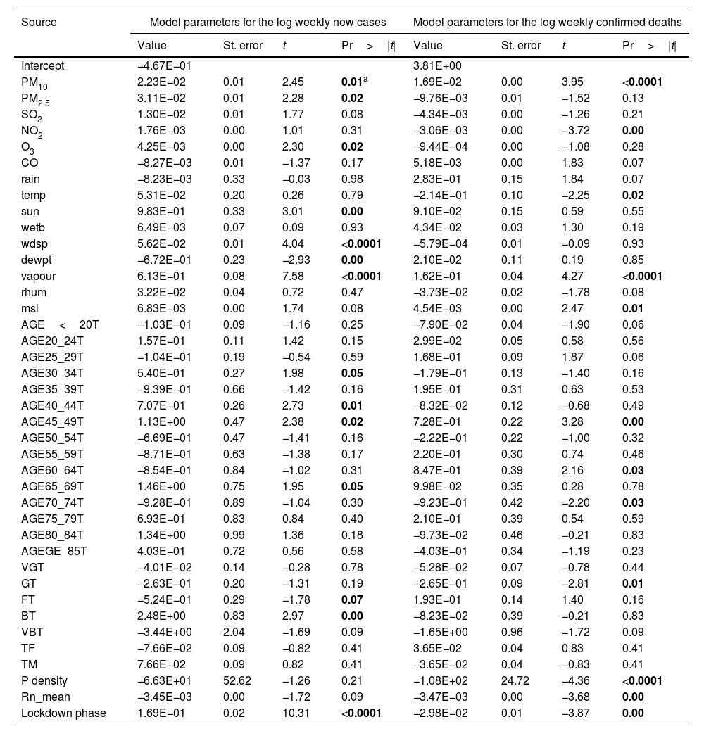
Table 2 gives vital details to the model parameters for the prediction of COVID-19 weekly new cases and deaths. This table is helpful for future predictions, or when it is needed to compare the coefficients of the model for given input data with the ones weekly observed (it could be used to compare the models for the prediction of COVID-19 weekly new cases and deaths). The p-value indicates the degree of significance, the lower the p-value of a variable, the stronger the effect in the model is anticipated. Subsequently, it is assumed that parameters with a p-value lower than 0.05 bring significant information to the prediction model. According to this assumption, PM10, PM2.5, O3, sun duration, vapour pressure, wind speed, dew point temperature, elder age category, and percent of the population in fair and bad health conditions together with lockdown are found to be the most significant parameters for the prediction of COVID-19 weekly new cases. This confirms the positive association between virus transmissions with some of the atmospheric pollutants and metrological parameters. This finding is in agreement with the few studies that have been recently conducted.7,9,10
Model parameters for prediction of COVID-19 weekly new cases and deaths.
| Source | Model parameters for the log weekly new cases | Model parameters for the log weekly confirmed deaths | ||||||
|---|---|---|---|---|---|---|---|---|
| Value | St. error | t | Pr>|t| | Value | St. error | t | Pr>|t| | |
| Intercept | −4.67E−01 | 3.81E+00 | ||||||
| PM10 | 2.23E−02 | 0.01 | 2.45 | 0.01a | 1.69E−02 | 0.00 | 3.95 | <0.0001 |
| PM2.5 | 3.11E−02 | 0.01 | 2.28 | 0.02 | −9.76E−03 | 0.01 | −1.52 | 0.13 |
| SO2 | 1.30E−02 | 0.01 | 1.77 | 0.08 | −4.34E−03 | 0.00 | −1.26 | 0.21 |
| NO2 | 1.76E−03 | 0.00 | 1.01 | 0.31 | −3.06E−03 | 0.00 | −3.72 | 0.00 |
| O3 | 4.25E−03 | 0.00 | 2.30 | 0.02 | −9.44E−04 | 0.00 | −1.08 | 0.28 |
| CO | −8.27E−03 | 0.01 | −1.37 | 0.17 | 5.18E−03 | 0.00 | 1.83 | 0.07 |
| rain | −8.23E−03 | 0.33 | −0.03 | 0.98 | 2.83E−01 | 0.15 | 1.84 | 0.07 |
| temp | 5.31E−02 | 0.20 | 0.26 | 0.79 | −2.14E−01 | 0.10 | −2.25 | 0.02 |
| sun | 9.83E−01 | 0.33 | 3.01 | 0.00 | 9.10E−02 | 0.15 | 0.59 | 0.55 |
| wetb | 6.49E−03 | 0.07 | 0.09 | 0.93 | 4.34E−02 | 0.03 | 1.30 | 0.19 |
| wdsp | 5.62E−02 | 0.01 | 4.04 | <0.0001 | −5.79E−04 | 0.01 | −0.09 | 0.93 |
| dewpt | −6.72E−01 | 0.23 | −2.93 | 0.00 | 2.10E−02 | 0.11 | 0.19 | 0.85 |
| vapour | 6.13E−01 | 0.08 | 7.58 | <0.0001 | 1.62E−01 | 0.04 | 4.27 | <0.0001 |
| rhum | 3.22E−02 | 0.04 | 0.72 | 0.47 | −3.73E−02 | 0.02 | −1.78 | 0.08 |
| msl | 6.83E−03 | 0.00 | 1.74 | 0.08 | 4.54E−03 | 0.00 | 2.47 | 0.01 |
| AGE<20T | −1.03E−01 | 0.09 | −1.16 | 0.25 | −7.90E−02 | 0.04 | −1.90 | 0.06 |
| AGE20_24T | 1.57E−01 | 0.11 | 1.42 | 0.15 | 2.99E−02 | 0.05 | 0.58 | 0.56 |
| AGE25_29T | −1.04E−01 | 0.19 | −0.54 | 0.59 | 1.68E−01 | 0.09 | 1.87 | 0.06 |
| AGE30_34T | 5.40E−01 | 0.27 | 1.98 | 0.05 | −1.79E−01 | 0.13 | −1.40 | 0.16 |
| AGE35_39T | −9.39E−01 | 0.66 | −1.42 | 0.16 | 1.95E−01 | 0.31 | 0.63 | 0.53 |
| AGE40_44T | 7.07E−01 | 0.26 | 2.73 | 0.01 | −8.32E−02 | 0.12 | −0.68 | 0.49 |
| AGE45_49T | 1.13E+00 | 0.47 | 2.38 | 0.02 | 7.28E−01 | 0.22 | 3.28 | 0.00 |
| AGE50_54T | −6.69E−01 | 0.47 | −1.41 | 0.16 | −2.22E−01 | 0.22 | −1.00 | 0.32 |
| AGE55_59T | −8.71E−01 | 0.63 | −1.38 | 0.17 | 2.20E−01 | 0.30 | 0.74 | 0.46 |
| AGE60_64T | −8.54E−01 | 0.84 | −1.02 | 0.31 | 8.47E−01 | 0.39 | 2.16 | 0.03 |
| AGE65_69T | 1.46E+00 | 0.75 | 1.95 | 0.05 | 9.98E−02 | 0.35 | 0.28 | 0.78 |
| AGE70_74T | −9.28E−01 | 0.89 | −1.04 | 0.30 | −9.23E−01 | 0.42 | −2.20 | 0.03 |
| AGE75_79T | 6.93E−01 | 0.83 | 0.84 | 0.40 | 2.10E−01 | 0.39 | 0.54 | 0.59 |
| AGE80_84T | 1.34E+00 | 0.99 | 1.36 | 0.18 | −9.73E−02 | 0.46 | −0.21 | 0.83 |
| AGEGE_85T | 4.03E−01 | 0.72 | 0.56 | 0.58 | −4.03E−01 | 0.34 | −1.19 | 0.23 |
| VGT | −4.01E−02 | 0.14 | −0.28 | 0.78 | −5.28E−02 | 0.07 | −0.78 | 0.44 |
| GT | −2.63E−01 | 0.20 | −1.31 | 0.19 | −2.65E−01 | 0.09 | −2.81 | 0.01 |
| FT | −5.24E−01 | 0.29 | −1.78 | 0.07 | 1.93E−01 | 0.14 | 1.40 | 0.16 |
| BT | 2.48E+00 | 0.83 | 2.97 | 0.00 | −8.23E−02 | 0.39 | −0.21 | 0.83 |
| VBT | −3.44E+00 | 2.04 | −1.69 | 0.09 | −1.65E+00 | 0.96 | −1.72 | 0.09 |
| TF | −7.66E−02 | 0.09 | −0.82 | 0.41 | 3.65E−02 | 0.04 | 0.83 | 0.41 |
| TM | 7.66E−02 | 0.09 | 0.82 | 0.41 | −3.65E−02 | 0.04 | −0.83 | 0.41 |
| P density | −6.63E+01 | 52.62 | −1.26 | 0.21 | −1.08E+02 | 24.72 | −4.36 | <0.0001 |
| Rn_mean | −3.45E−03 | 0.00 | −1.72 | 0.09 | −3.47E−03 | 0.00 | −3.68 | 0.00 |
| Lockdown phase | 1.69E−01 | 0.02 | 10.31 | <0.0001 | −2.98E−02 | 0.01 | −3.87 | 0.00 |
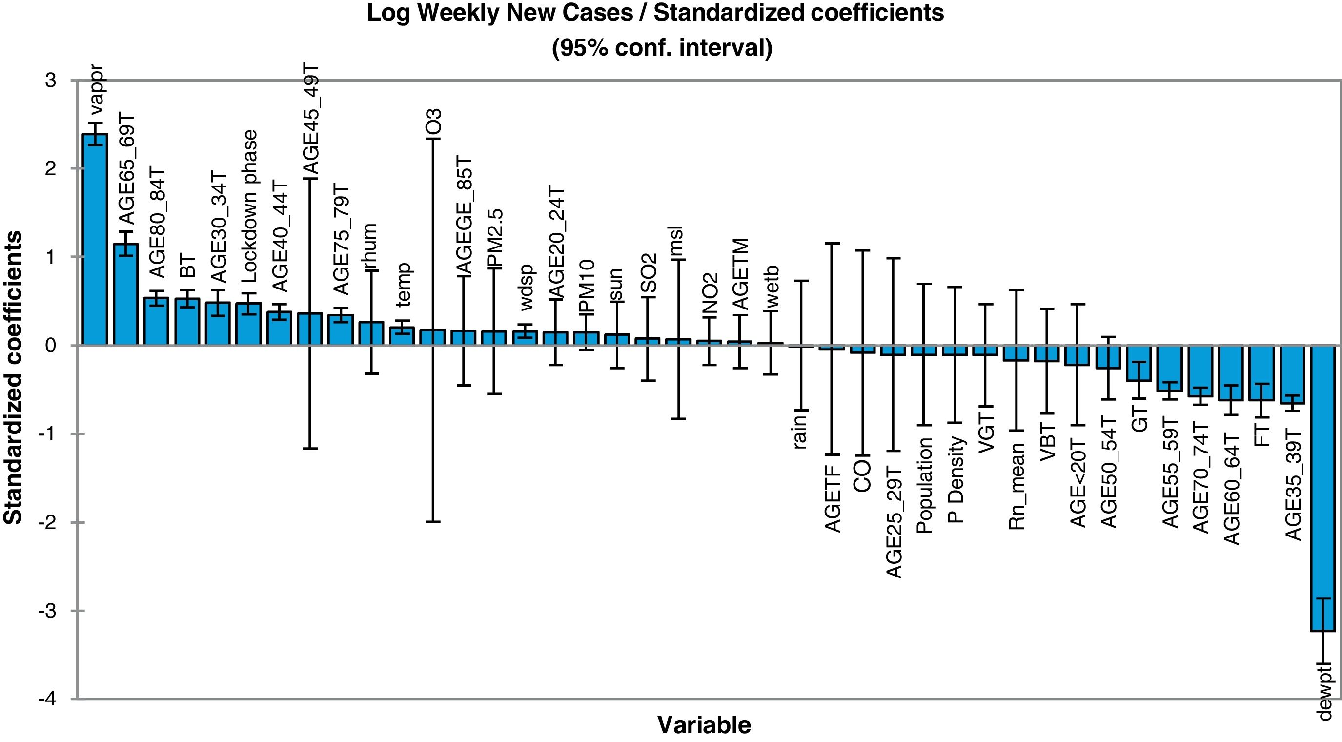
Concerning the model for prediction of weekly deaths, PM10, temperature, vapour and mean sea level pressures, elder age category, percent of the population with a good health condition, background radon levels together with population density and locking down are found to be the most dependable parameters. It is also clear that the mean radon concentration has a positive effect on the increase of virus lethality. The mathematical equation of the model's parameters, which can be also used for future predictions (in the case of the inputs being provided), can be obtained using the coefficients reported in Table 2. In other words, the values of this table are the regression coefficient of (b1, b2, … and b41) and the a constant is the intercept value. Note that back-transformation of calculated logarithmic values to the original scale is also necessary. In order to have a better understanding of the effect of explanatory parameters on COVID-19 contagion and lethality rates, Fig. 3 and Figure S-5 (Appendix C) show the standardized regression coefficients, sometimes referred to as beta coefficients.

Fig. 3 and Figure S-5 (Appendix C) allow us to directly compare the relative influence of the explanatory variables on the dependent variable, and their significance. According to these figures, dew point temperature (negative correlation) and vapour pressure (positive correlation) have the highest standardized significances in the model for the prediction of contagion. In the model for the prediction of lethality rates, temperature (negative correlation), and vapour pressure (positive correlation) showed the highest significance levels.
Model validityThe results of cross-validation of observed and predicted models (see S-4 (Appendix C) show that the predicted values match those measured. In fact, the absolute mean prediction error weekly COVID-19 new cases (NC) and confirmed deaths (CD) (MAENC=0.38 and MAECD=0.15) and the Standard Error of Mean (SEMNC=0.0007 and SEMCD=0.0003) are close to zero, indicating that the prediction method of both contagion and lethality rates are unbiased (centred on the true values) and the model is noticeably accurate. Additionally, the average standard error (SECD=0.14) is less than the root mean squared error (RMSECD=0.23), suggesting that the prediction model slightly underestimates the lethality rates. However, SENC (=0.77) is more than RMSENC (=0.50) which indicates that the model overestimates the contagion rates. The computed RMSEs and MSEs of Log transformed weekly COVID-19 new cases (NC) and confirmed deaths (CD) predicted for Irish counties are shown in Table S-5 (Appendix C). The range of the errors for the PCR-NC model was 0.13 (for County Kerry) to 0.52 (for County Dublin), while the errors for PCR-CD ranged from 0.35 (for County Dublin) to 0.58 (for County Waterford). Based on the obtained values, it is found that the error of the model for the prediction of contagion rates is slightly higher than the lethality prediction model.
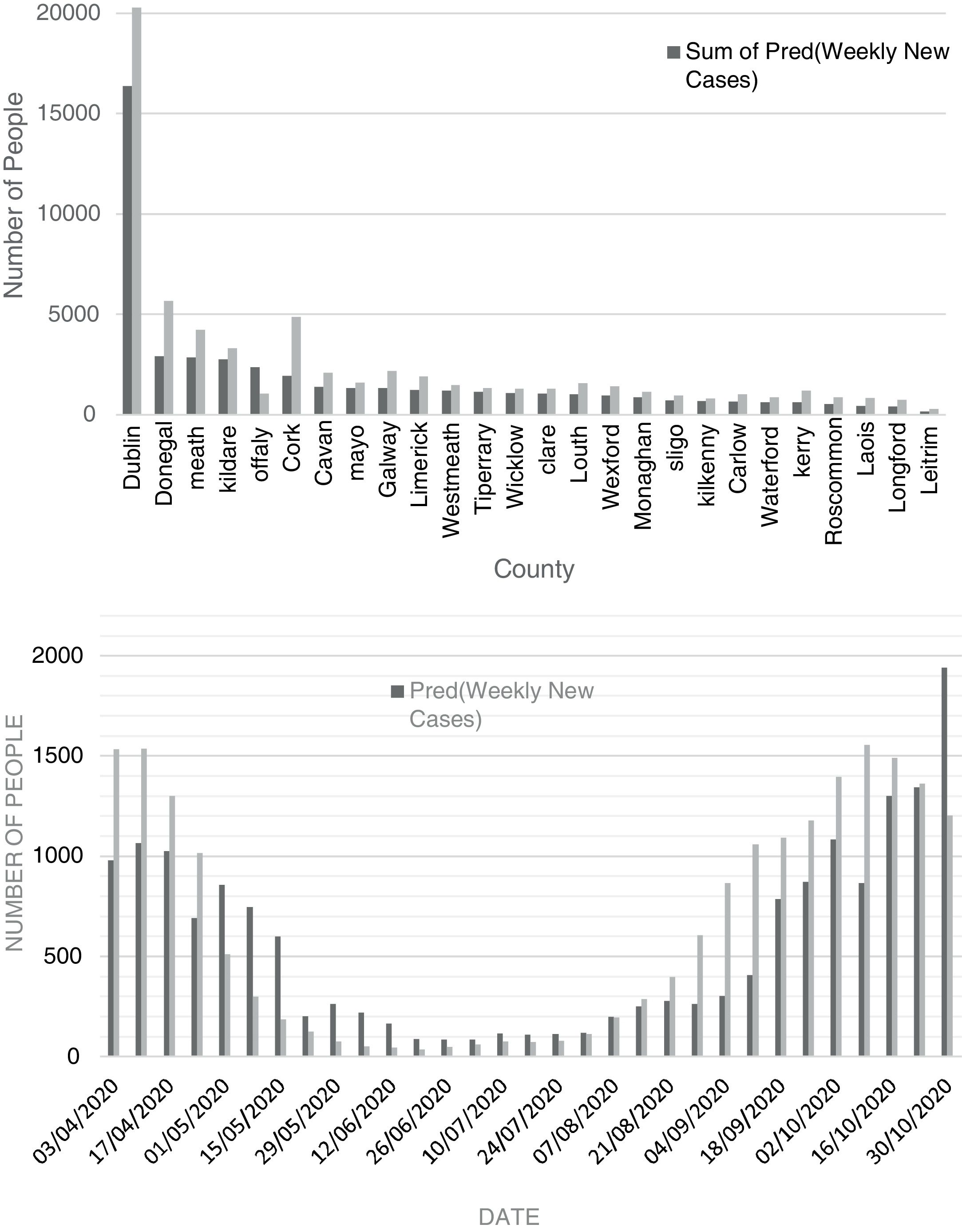
Comparison of observed and predicted weekly new cases and deaths of COVID-19 in Dublin County and the other Irish CountiesFig. 4 (top) shows the total number of new cases observed and predicted for the study period (3 April to 30 October 2020). According to this figure, the number of predicted values, for most of the Irish counties, is less than the observed cases. This reveals that there may be some hidden factors affecting the contagion rates that were not considered in this study, one of them could be the very high contagiousness of the SARS-CoV-2 virus in hospitals where healthcare workers were infected. The average difference between the predicted and observed values was found to be around 27%. Also, the cumulative percent of contagion rate of health workers for the same period was about 18% showing extreme contagiousness of the virus in sanitary environments which would account for most of the difference between predicted and observed cases. Another parameter that would explain the remainder of the difference is the actual degree of social distancing considered by the majority of the population.
 and observed weekly new cases in County Dublin (bottom) (3 April to 30 October).")
According to Figure S-6 (Appendix C), except for county Dublin, the total predicted and observed deaths due to COVID-19 from 03 April to 30 October 2020 are close to each other (predicted values are slightly lower). The excess deaths in County Dublin can be attributed to the residential and community care facilities including nursing homes for which significantly high death rates (62% total) were reported. Also, the cumulative death rate percent of health workers for the period of study was about 1%. As can be seen in Figure S-7 (Appendix C), the total predicted death for the county of Dublin is 37% of the observed ones. As most of the care facilities and hospitals are in County Dublin, it can be concluded that the additional deaths from health care facilities together with the death of health workers in hospitals can justify the high difference between the observed and predicted deaths (63% total).
Fig. 4 (bottom) shows the chart of predicted and observed weekly cases of COVID-19 in County Dublin. There is a rather good agreement between predicted and observed cases. In this figure, one can observe that the number of predicted cases for the period after late October tends to overestimate the number of new cases. This is likely related to the restrictive measures set by the government to control the second wave leading to a decrease in the number of new cases. According to Figure S-7 (Appendix C), except for April and May 2020, the predicted values are close to the observed ones. High numbers of deaths (most of them attributed to healthcare facilities) in April and early May were suppressed as a result of preventive activities of the Department of Health of Ireland.
DiscussionPredicting the contagion and lethality of COVID-19 is a multifaceted endeavour, hinging on a comprehensive examination of various interconnected variables. These variables can be broadly categorized into three primary domains: epidemiological, biological, and socio-demographic factors. Epidemiological factors include fundamental metrics such as the basic reproduction number (R0), which quantifies the virus's contagiousness, along with the incubation period and the extent of asymptomatic or presymptomatic transmission. These metrics are critical for understanding contagion dynamics, while the case fatality rate (CFR) offers insights into the virus's lethality. Biological factors encompass viral attributes like viral load and genetic variations or strains, coupled with host-specific factors such as immune responses, comorbidities, age, and vaccination status. Together, they shape the severity of the disease and its potential to spread. Socio-demographic factors, such as population density, healthcare infrastructure, behavioural compliance, travel patterns, healthcare access, and public health interventions, further modulate the pandemic's trajectory in specific regions.
To produce future prediction models for COVID-19 contagion and lethality, these variables serve as the cornerstone for data-driven analyses. Machine learning and epidemiological modelling techniques harness these variables to create predictive models that integrate historical data to identify patterns and relationships. These models enable us to estimate future contagion rates, disease spread trajectories, and potential lethality. By closely monitoring viral variants and comprehending their impact on transmission and severity, models can adapt in real time to anticipate changes in the virus's behaviour. Furthermore, public health interventions and vaccination campaigns can be fine-tuned based on these predictions to curtail the virus's spread and reduce its lethality. The ongoing collaboration between scientists, epidemiologists, and data analysts is essential for refining and improving these prediction models for COVID-19, ensuring that policymakers have accurate and actionable information to make informed decisions and effectively combat the pandemic.
Conclusions and implicationThis paper studied the spatial correlations between atmospheric pollution, weather information, and social-demographic data with contagion and lethality rates of COVID-19 in Ireland. This country was selected for our study due to the extensive use of a large number of health and non-health technologies including extensive monitoring, diagnostic testing and the use of medications to stop the spread of COVID-19. Given this, we were able to collect a comprehensive set of data which allowed us to study the relationship between environmental and climatic variables and the COVID-19 pandemic in order to have a better understanding of the parameters that might affect its contagiousness and killing power. According to the correlation circle of the factors (Table 1) which is a result of principal components analysis (PCA), two sets of parameters were identified; (1) those affect health conditions like ageing and health status, and (2) those affect the spread of the virus such as temperature and humidity. A principal components regression analysis was carried out to (a) develop a prediction model and (b) evaluate the contribution of input parameters on the virus transmission and its lethality. As a result of this study, it was found out atmospheric pollution contributes in two ways; (a) by facilitating virus transmission and (b) to a lesser extent by forcing extra pressure on the respiratory system (e.g. background radon activity). The metrological parameters, especially air temperature and dew point temperature, were found to significantly affect both contagiousness and mortality. In alignment with our anticipations, the elderly category was found to be the most vulnerable group to be infected by the virus. Health status as an indicator of the well-being of the immune system was found to have a key role in fighting against the virus and decreasing the lethality rate. We have also found that the lockdown set by the Irish government significantly prevented the increase in COVID-19 cases.
Additionally, we acknowledge the importance of epidemiological knowledge for primary care physicians. The variables influencing transmission and prognosis, such as age, temperature, and wind speed, may not be directly modifiable by healthcare professionals, but understanding these factors is indeed valuable for informed decision-making in primary care settings. This insight can aid healthcare providers in better managing patient care and public health strategies.
The models we developed were successful in predicting a portion of contagion and lethality rates related to environmental and sociodemographic factors. However, it seems that there are additional effective parameters that were not included in this study since the input parameters introduced in our model do not cover the whole variation in the predictions. Therefore suggest adding parameters such as the number of deaths in care homes, percent of cumulative contagion and mortality among health workers, the degree of compatibility with social distancing, blood groups, details about the number of tests per capita and most importantly the vaccination rates while developing future models.
Institutional review board statementNot applicable.
Data availabilityPlease see the link: https://zenodo.org/record/7816909#.ZDUbr3bMLRY.
Conflicts of interestThe authors declare no conflict of interest.
The authors would like to thank the Irish Government, the Department of Health, the Environmental Protection Agency, and Met Éireann as the sources of the raw data used as input for the prediction model. We would like to also acknowledge Conor Rothwell for his contribution to curating the metrological dataset. We thank Bernd Saurugger from the European Open Science Cloud (EOSC) for his useful discussions and help. This work was supported by the European Open Science Cloud (EOSC). EOSC secretariat has received funding from the European Union's Horizon Programme call H2020-INFRAEOSC-05-2018-2019, Grant Agreement number 831644.
The following are the supplementary data to this article: