

The particular development of the Italian regional disparities and North–South inequality is correlated with the structural change which came about during the process of industrialisation. This process began in certain Northern poles producing a sudden increase in regional inequality, but, as it later spread through the North and Centre, a fall in regional disparities resulted. Industrialisation only superficially interested the South, which remained relatively backward. While regional convergence occurred both within the North and the South, divergence between North and South persisted. After presenting series of both labour force in industry and regional GDP, we analyse the relationship between industrialisation and inequalities and, finally, quantify the importance of the North–South dualism within the context of the Italian regional disparities.
La peculiar tendencia de la disparidad regional en Italia, y la diferencia entre Norte y Sur, están relacionadas con el cambio estructural determinado por el proceso de industrialización. Esta empezó en algunos polos del Norte produciendo un rápido incremento de las desigualdades regionales; sucesivamente se extendió a otras áreas del Norte y del Centro, determinando una convergencia regional; se extendió limitadamente en el Sur, que permaneció relativamente atrasado, aunque hubo una breve fase de recuperación, verificada durante los años 60. Mientras la convergencia regional se verificó tanto en el Norte como en el Sur, la diferencia entre las 2 áreas permaneció amplia. En este artículo, tras haber presentado los datos referentes a la fuerza laboral en la industria y el PIB regional, analizamos la relación entre industrialización y diversidad de desarrollo, cuantificando, al final, la importancia del dualismo Norte-Sur en el contexto del desequilibrio entre las regiones italianas.
The evolution of regional inequality during the process of economic development is a central topic of interest and debate (World Bank, 2009). In a seminal study, using cross-section and time series for some nations, Williamson (1965) showed that regional inequality follows an inverted U-curve, increasing in a first stage of national development and later decreasing. Williamson suggested that this particular trend of spatial inequality was determined by some key factors: interregional labour and capital movements, government policies, and interregional linkages that influence the diffusive effects of technological and social change. These factors, which initially cause divergence on regional income, in a more advanced stage of national development have a re-equilibrating effect, thus determining convergence. According to Alonso (1980), the bell-shaped curve of regional inequality represents one of the main features in the process of economic development. However, since economic growth is a continuous process, regional convergence may be followed by divergence in a later phase: hence the dynamic of regional inequality describes an inverted-S rather than an inverted U curve (Amos, 1988; Fan and Casetti, 1994).
Due to the scarcity of regional historical data over long periods, the relationship between regional inequalities and development has been investigated mainly on the basis of cross-sectional data on economies at diverse levels of development (Barrios and Strobl, 2009), or through time series for relatively short periods (Ezcurra and Rapún, 2006). Some international studies covering long periods are, however, available. With reference to the USA, Kim (1998) showed the existence of a long-term inverted U-pattern in regional inequality, especially in the manufacturing sector. For France, series of value added, population and labour force from 1860 show the existence of a bell-shaped curve in spatial development (Combes et al., 2011). Regional inequality in Spain also followed an inverted-U trajectory, increasing during the early phases of economic growth and industrialisation in relationship with the distribution of industry and services (Rosés et al., 2010; Martinez-Galarraga, 2012). In Portugal, regional inequalities described a similar trend during the period between 1890 and 1980, reaching a peak around 1970, as a consequence of the concentration of industry and services (Badia-Miró et al., 2012). A different pattern characterised Sweden, where regional inequality diminished from 1860 to 1980, but increased over the following twenty years; hence without any bell shaped trend (Enflo and Ramón-Rosés, 2012). The case of Belgium, investigated by Buyst (2011), shows a similar picture during the period 1892–2000: a first long phase of convergence among the provinces was followed, after the 1960s, by a phase of divergence.
Italy represents an important case study for the analysis of the evolution of regional inequalities and their relation to national development and industrialisation. The availability of estimates on GDP per region from the end of the Nineteenth century, and a recent revision and updating of series of labour force at the regional level, for the period 1861–2001, clarify the changes in both the regional product and the labour force over a period of one century (Daniele and Malanima, 2007, 2011, forthcoming).1 Since modern growth only started in Italy in the last decades of the Nineteenth century, available data allow a deeper understanding of the long transition from the traditional agricultural system to the industrial and finally post-industrial systems. The present day existence of a wide North–South divergence contributes to the interest of the Italian case-study for both historians and economists. In 2011, GDP per capita in the South was, in fact, 58 percent of that in the Centre-North (Istat, 2013; Svimez, 2012).
This paper examines the long-term evolution of regional disparities in Italy. Exploiting new data on labour force and GDP, it relates regional inequalities to the process of geographic concentration-dispersion of industry. Our view is that regional inequality in Italy described an inverted U-curve and that this trend was related to the changes that occurred during the process of economic modernisation. Industrialisation began in some Northern poles and produced a sudden increase in regional inequality, later spreading through the North and Centre with a resultant fall in regional disparities; it superficially interested the South, which remained relatively backward with only a modest and short-lived economic recovery during the 1960s. While convergence occurred both within the North and the South, divergence between North and South persisted. In fact, North–South economic inequality rose from the end of the Nineteenth century, only easing off for a short period during the 1960s. The recent development of the Italian post-industrial economy was characterised by oscillations in North–South inequality on a high level and without a clear trend.
In the second section of this paper, we recall the evolution of the regional disparities in industrialisation (proxied by the labour force in industry) and GDP. In the third section, we present a statistical analysis in order to examine the relationship between structural change and regional inequality. In the fourth section, we analyse North–South inequality within the context of regional disparities.
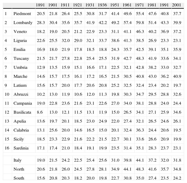
2Industrial labour force and regional GDP: the data2.1The labour forceTable 1 shows the percentage of labour force in industry as compared to the total labour force per region in the period 1891–2001. Since we can only avail of yearly regional data on labour force in standard labour units from the 1980s, elaborated by the Italian national statistical institute (Istat), a long-term reconstruction is only possible by means of the population censuses, held in Italy every decade since 1861.2
Percentage of the industrial labour force per region out of the total labour force 1891–2001.
| 1891 | 1901 | 1911 | 1921 | 1931 | 1936 | 1951 | 1961 | 1971 | 1981 | 1991 | 2001 | ||
| 1 | Piedmont | 20.5 | 21.8 | 26.4 | 25.5 | 30.8 | 31.7 | 41.4 | 49.6 | 55.4 | 47.6 | 40.8 | 37.7 |
| 2 | Lombardy | 28.3 | 30.4 | 35.6 | 35.7 | 41.9 | 42.2 | 49.2 | 57.4 | 59.8 | 51.4 | 43.3 | 39.9 |
| 3 | Veneto | 18.2 | 19.0 | 20.5 | 21.2 | 22.9 | 23.3 | 31.1 | 41.1 | 46.3 | 40.2 | 36.9 | 37.2 |
| 4 | Liguria | 22.6 | 25.5 | 32.0 | 29.0 | 32.1 | 33.7 | 38.6 | 41.3 | 38.5 | 26.9 | 23.3 | 23.1 |
| 5 | Emilia | 16.9 | 18.0 | 21.9 | 17.8 | 18.5 | 18.8 | 24.3 | 35.7 | 42.5 | 39.1 | 35.1 | 35.9 |
| 6 | Tuscany | 21.5 | 21.7 | 27.8 | 22.8 | 25.4 | 25.5 | 31.9 | 42.7 | 48.3 | 41.9 | 33.6 | 34.1 |
| 7 | Umbria | 12.9 | 13.5 | 15.9 | 15.1 | 16.6 | 17.1 | 22.5 | 32.1 | 42.8 | 38.2 | 33.0 | 32.7 |
| 8 | Marche | 14.6 | 15.7 | 17.5 | 16.1 | 17.2 | 16.5 | 21.5 | 30.5 | 40.8 | 43.0 | 36.2 | 40.9 |
| 9 | Latium | 15.6 | 15.7 | 20.0 | 17.7 | 20.6 | 20.8 | 25.2 | 32.5 | 32.4 | 23.4 | 20.2 | 19.7 |
| 10 | Abruzzi | 10.2 | 13.0 | 11.9 | 10.6 | 12.0 | 11.3 | 19.8 | 30.3 | 34.7 | 29.5 | 28.8 | 32.6 |
| 11 | Campania | 19.0 | 22.8 | 23.6 | 21.6 | 23.1 | 22.6 | 27.0 | 34.0 | 38.1 | 28.8 | 24.0 | 24.4 |
| 12 | Basilicata | 8.6 | 13.0 | 12.1 | 11.5 | 13.1 | 11.9 | 15.0 | 26.5 | 34.1 | 27.1 | 25.9 | 34.6 |
| 13 | Apulia | 13.6 | 19.7 | 20.1 | 18.5 | 23.0 | 24.9 | 22.0 | 27.4 | 32.1 | 26.5 | 24.6 | 26.1 |
| 14 | Calabria | 13.1 | 25.6 | 20.0 | 14.6 | 16.5 | 15.0 | 20.1 | 32.4 | 36.3 | 24.4 | 20.6 | 19.5 |
| 15 | Sicily | 18.5 | 23.3 | 22.9 | 21.6 | 22.2 | 21.5 | 22.7 | 30.1 | 33.6 | 26.6 | 20.9 | 19.9 |
| 16 | Sardinia | 17.1 | 17.4 | 21.0 | 18.4 | 19.1 | 19.9 | 23.5 | 31.4 | 35.1 | 28.3 | 23.7 | 23.1 |
| Italy | 19.0 | 21.5 | 24.2 | 22.5 | 25.4 | 25.6 | 31.0 | 39.8 | 44.1 | 37.2 | 32.0 | 31.8 | |
| North | 20.6 | 21.8 | 26.0 | 24.5 | 27.8 | 28.1 | 34.9 | 44.1 | 48.3 | 41.6 | 35.7 | 34.8 | |
| South | 15.6 | 20.8 | 20.3 | 18.2 | 20.0 | 19.8 | 22.7 | 30.8 | 35.0 | 27.4 | 23.5 | 24.2 | |
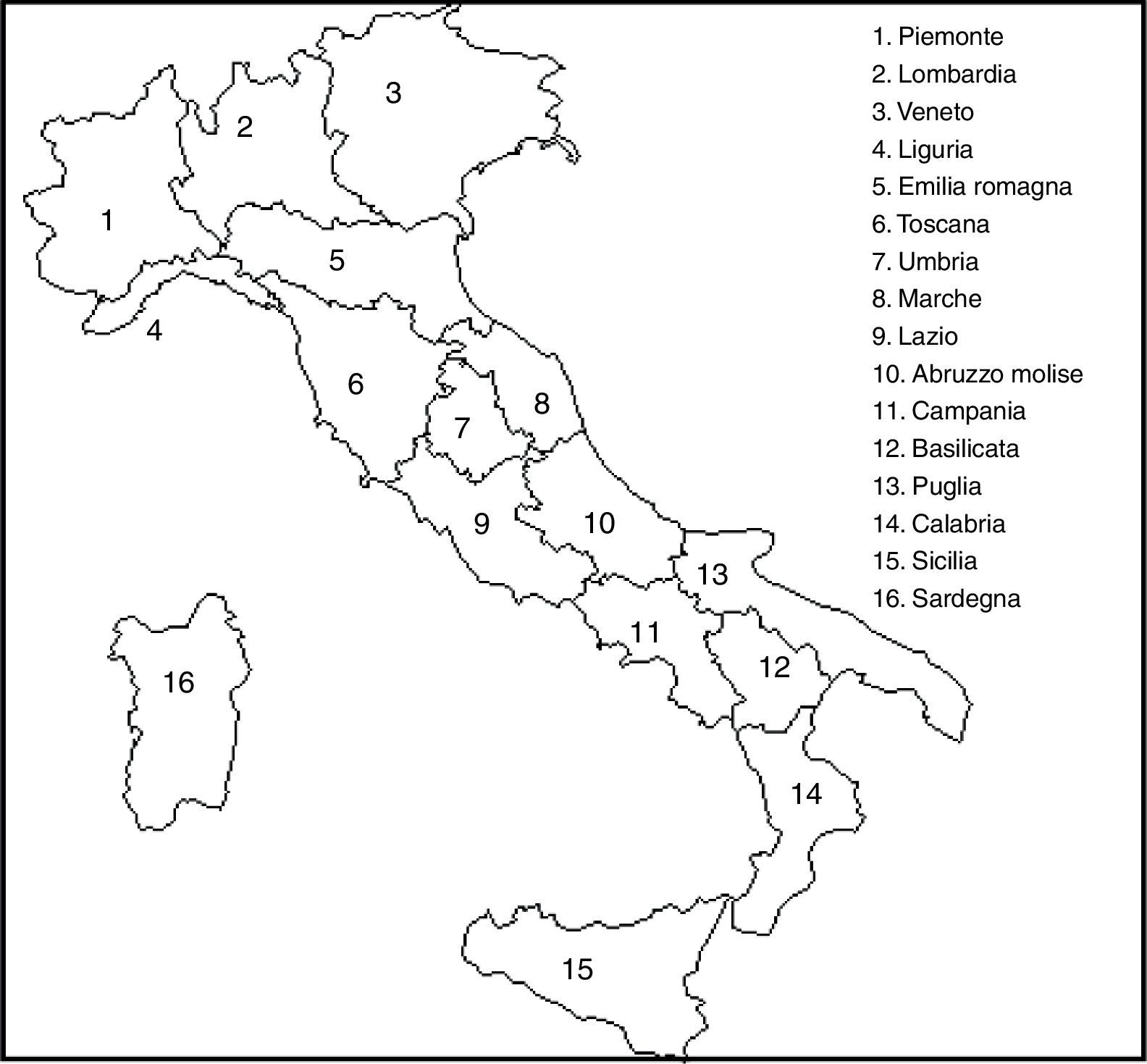
Note: North or Centre-North: regions 1-9; South or South-Islands: regions 10-16. Piedmont including Val d’Aosta, Veneto including Friuli Venetia Giulia and Trentino Alto Adige; Abruzzi including Abruzzo and Molise. Fig. 1.A. in the Appendix shows a map of the Italian regions. On the labour force see also Broadberry et al. (2011).
In 1861, the employment structure in Italy was still that typical of pre-industrial economies. The main share of the labour force (64 percent) worked in agriculture while the rest was equally distributed between industry and services (Daniele and Malanima, forthcoming). In the first decade after national Unification, there was not yet a clear difference in industrialisation between the North and South of Italy. Even though in Lombardy and, to a lesser extent, in Piedmont, Emilia and Tuscany, the industrialisation levels were higher than the Italian average, some Southern regions, such as Sicily and Campania, also presented relatively high shares of workers in industry (Bevilacqua, 1993; Fenoaltea, 2001, 2006; Ciccarelli and Fenoaltea, 2012). An industrialised North and a de-industrialised South did not yet exist.
In 1891, the Italian economy was still relatively backward, as the structural distribution of the labour force indicates (Fig. 1). Industry employed 19 percent of the labour force: 21 percent in the North and 16 percent in the South. Indirect evidence of the relative backwardness of the economic structure is provided by figures regarding international emigration. Between 1876 and 1900, about 5,250,000 Italians emigrated, 71 percent of which were from the North and Centre (Svimez, 1961, p. 123). The highest numbers of emigrants originated from the regions of Veneto, Venetia Giulia and Piedmont; that is from some relatively underdeveloped areas of the North. After 1900, the flow or emigrants from Southern regions became prominent (Sanfilippo, 2001, p. 79), as soon as the Mezzogiorno began losing ground in the process of economic modernisation.
 and, for 1861, Maic (1886).")
Modern growth started in Italy during the 1880s (Fenoaltea, 2003b, 2006). From then on, the share of the industrial labour force in the North increased significantly, reaching 26 percent in 1911, while in the South it was around 20 percent. In 1911, the relative level of industrialisation in the North–West area, the so-called “industrial triangle” between Genoa, Milan and Turin, was significantly higher than the national average (Zamagni, 1978). In Lombardy, the industrial labour force already exceeded 35 percent; in Liguria it was 32 percent. The concentration of industry in the North increased between the First and the Second World Wars. In the period spanning 1901–1931, only six regions exceeded 10 percent of population employed in the secondary sector: Lombardy, Piedmont, Veneto, Liguria, Emilia and Tuscany.3
Several factors, such as a better infrastructural endowment, and a relatively higher level of literacy have been indicated as favourable preconditions for the formation of an industrial base in the North–West. The availability of water power, crucial for the proto-industrial production of silk (especially in Lombardy), a large domestic market and the geographic proximity to developing European markets played major roles for the location of industry in the North–West (A’Hearn and Venables, 2013). On the contrary, the small domestic market, the great distance from large foreign markets worsened by the lack of infrastructures, negatively impacted on transport costs and hampered industrial location in the Southern regions.4 The effect of geography was crucial, perhaps more than in other countries, in determining the North–South imbalance. Italy has, in fact, a peculiar geography: Northern regions are close to the core regions of Europe, while the South is a European periphery distant 1300km from the Northern borders of the country.
The two decades after the Second World War was the period when “unlimited” labour supply in agriculture began to be increasingly employed in industry and services (Kindleberger, 1967). In Italy, the reallocation of the labour force occurred both between sectors and between regions: during the period 1951 and 1971 more than 4 million people migrated from the South towards the North (Del Monte and Giannola, 1978, pp. 167–170). In this period, both the North-East and Central regions were involved by an intense process of industrialisation, characterised by clusters – the “industrial districts” – of small and medium enterprises (Brusco and Paba, 1997). The spread of industry towards the regions of “new” industrialisation notably changed the economic geography of Italy. Industrialisation increased in the South, as well, although the differences with the most developed Northern regions continued to be remarkable. In 1981, in the North, 42 percent of the labour force was employed in industry. In the South, it hardly exceeded 27 percent. Italy was a dualistic economy (Fig. 2). At the start of the Twenty First century, a difference of 10 percentage points in the industrial participation rate still existed.5
.")
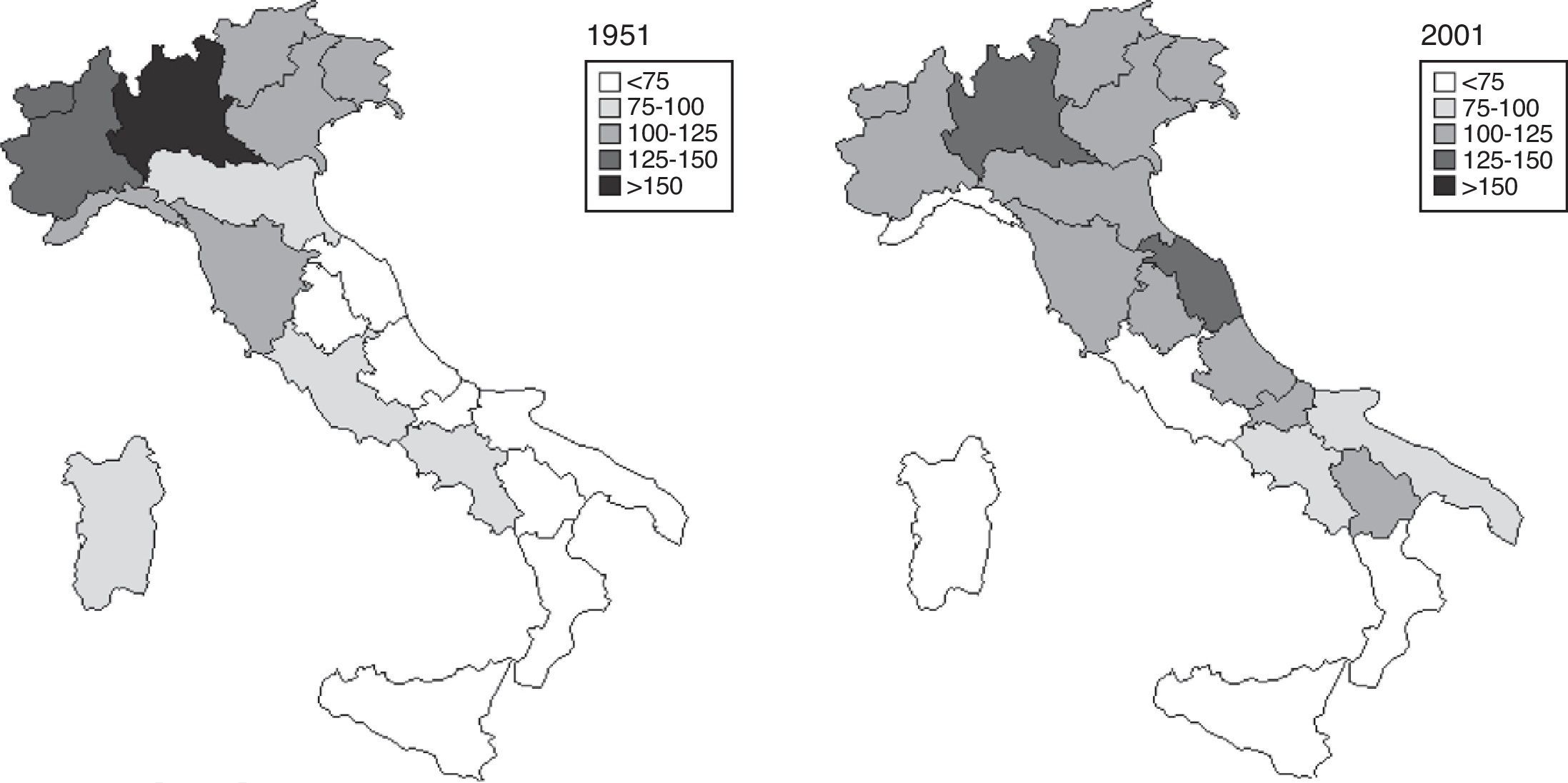
The process of concentration-dispersion of industry, which occurred in Italy during the Twentieth century, can be summarised by the Ellison–Glaeser index of concentration of the industrial labour force:
where L represents industrial occupation in region i and a the surface, both expressed as ratios respectively of the total industrial labour force and the extent of the country (Ellison and Glaeser, 1997; Gardiner et al., 2011). The trend clearly describes an inverted U curve (Fig. 3). The apex is reached immediately after World War 2. In 2001, the level of industrial concentration was not significantly higher than that of one hundred years before.2.2Regional GDP

Until about 1880, when industrial output began to rise relative to agriculture (Fenoaltea, 2003a, 2003b, 2005), more than 50 percent of Italian GDP came from the primary sector. As in any agrarian economy, the Italian per capita GDP was relatively low: in 1861, it was about 2000 Euros (2010 purchasing power).6
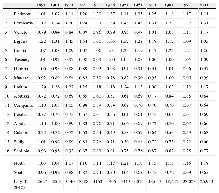
It is hard to specify the degree of regional inequality until 1891, when our series of regional per capita GDP start. Regional disparity was relatively low at that time, certainly much lower than today. Both in the South and the North there were prosperous and poor regions and, within these regions, prosperous and poor areas. Table 2 presents our series of regional per capita GDP.
Regional per capita GDP 1891–2001 (Italy=1) and per capita GDP in Italy (2010 euros).
| 1891 | 1901 | 1911 | 1921 | 1931 | 1936 | 1951 | 1961 | 1971 | 1981 | 1991 | 2001 | ||
| 1 | Piedmont | 1.01 | 1.07 | 1.14 | 1.20 | 1.30 | 1.37 | 1.41 | 1.35 | 1.25 | 1.18 | 1.17 | 1.11 |
| 2 | Lombardy | 1.12 | 1.14 | 1.20 | 1.24 | 1.33 | 1.39 | 1.48 | 1.43 | 1.31 | 1.23 | 1.32 | 1.31 |
| 3 | Veneto | 0.79 | 0.84 | 0.84 | 0.89 | 0.96 | 0.99 | 0.95 | 0.97 | 1.01 | 1.08 | 1.11 | 1.17 |
| 4 | Liguria | 1.22 | 1.31 | 1.45 | 1.54 | 1.60 | 1.65 | 1.32 | 1.28 | 1.18 | 1.12 | 1.09 | 1.03 |
| 5 | Emilia | 1.07 | 1.08 | 1.09 | 1.07 | 1.06 | 1.04 | 1.23 | 1.19 | 1.17 | 1.25 | 1.21 | 1.26 |
| 6 | Tuscany | 1.01 | 0.97 | 0.97 | 0.98 | 0.99 | 1.00 | 1.04 | 1.08 | 1.06 | 1.09 | 1.05 | 1.09 |
| 7 | Umbria | 1.06 | 0.98 | 0.88 | 0.89 | 0.92 | 0.93 | 0.91 | 0.91 | 0.91 | 1.01 | 0.96 | 0.97 |
| 8 | Marche | 0.92 | 0.89 | 0.84 | 0.82 | 0.80 | 0.78 | 0.87 | 0.90 | 0.95 | 1.00 | 0.95 | 0.99 |
| 9 | Latium | 1.29 | 1.26 | 1.22 | 1.25 | 1.18 | 1.16 | 1.24 | 1.13 | 1.08 | 1.07 | 1.12 | 1.17 |
| 10 | Abruzzi | 0.72 | 0.72 | 0.69 | 0.65 | 0.60 | 0.57 | 0.61 | 0.69 | 0.77 | 0.84 | 0.85 | 0.84 |
| 11 | Campania | 1.10 | 1.08 | 1.05 | 0.98 | 0.89 | 0.84 | 0.69 | 0.70 | 0.70 | 0.70 | 0.67 | 0.64 |
| 12 | Basilicata | 0.77 | 0.76 | 0.73 | 0.67 | 0.61 | 0.56 | 0.61 | 0.61 | 0.73 | 0.68 | 0.64 | 0.69 |
| 13 | Apulia | 1.10 | 1.00 | 0.89 | 0.83 | 0.76 | 0.71 | 0.66 | 0.69 | 0.72 | 0.70 | 0.67 | 0.66 |
| 14 | Calabria | 0.72 | 0.72 | 0.72 | 0.63 | 0.54 | 0.49 | 0.58 | 0.57 | 0.64 | 0.59 | 0.59 | 0.63 |
| 15 | Sicily | 1.01 | 0.96 | 0.89 | 0.83 | 0.76 | 0.71 | 0.59 | 0.64 | 0.72 | 0.75 | 0.72 | 0.66 |
| 16 | Sardinia | 0.98 | 0.96 | 0.93 | 0.87 | 0.83 | 0.81 | 0.75 | 0.76 | 0.87 | 0.82 | 0.75 | 0.77 |
| North | 1.03 | 1.04 | 1.07 | 1.10 | 1.14 | 1.17 | 1.21 | 1.19 | 1.15 | 1.15 | 1.16 | 1.18 | |
| South | 0.96 | 0.92 | 0.88 | 0.82 | 0.74 | 0.70 | 0.64 | 0.67 | 0.72 | 0.72 | 0.69 | 0.67 | |
| Italy (€ 2010) | 2627 | 2865 | 3440 | 3588 | 4163 | 4495 | 5349 | 9074 | 13,647 | 18,637 | 23,023 | 26,943 | |
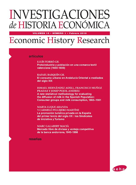
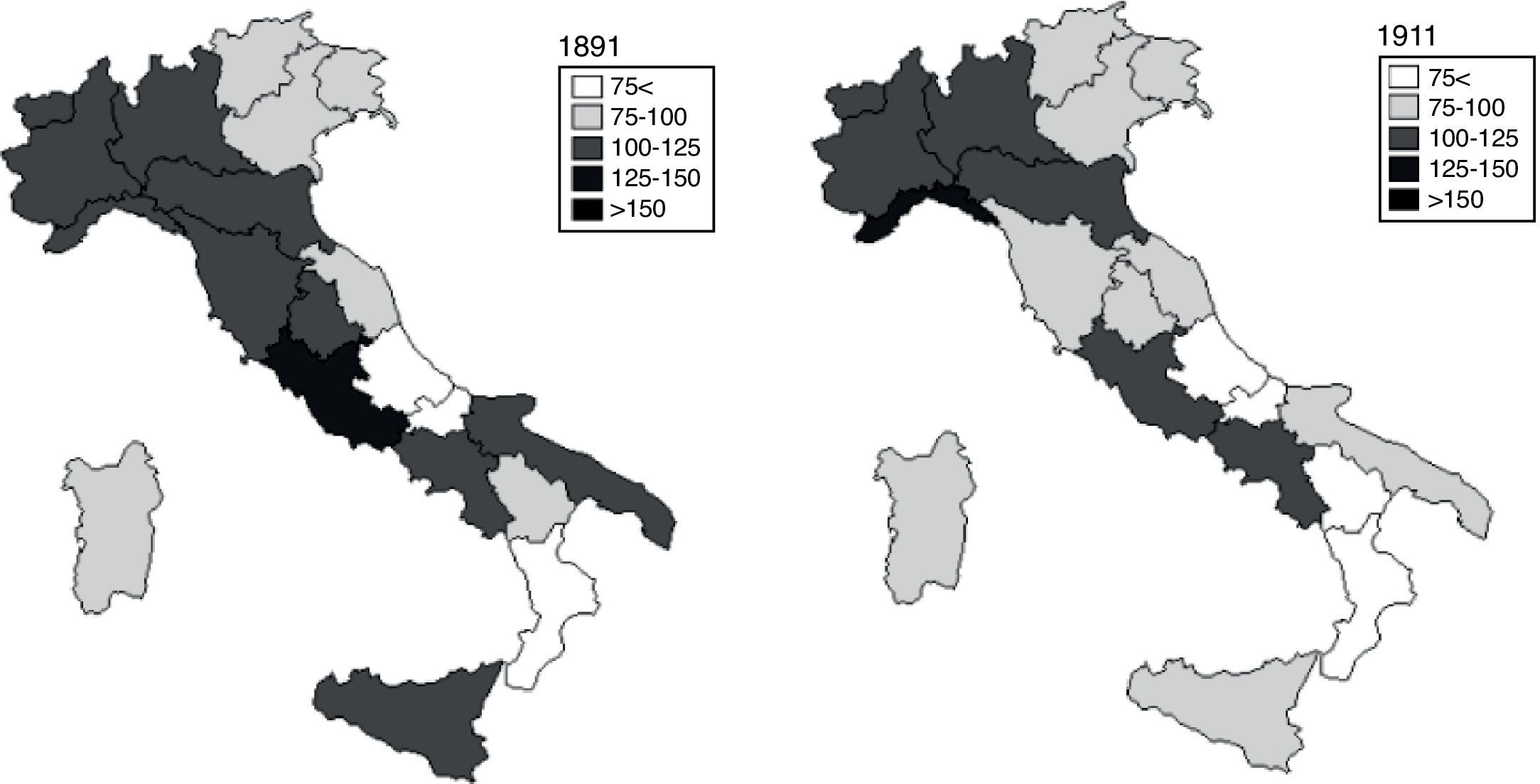
We see that, in 1891, per capita income in the North-West regions – Piedmont, Lombardy and Liguria – exceeded the national average. Certain regions of the South were also relatively prosperous. Campania and Apulia were just below the level of Lombardy, whilst on the main islands, Sicily and Sardinia, per capita output was close to the national average. Abruzzi, Calabria and Basilicata lagged behind. The Northeast, including Veneto, Trentino and Friuli Venetia Giulia, was relatively backward. Almost all regions to the East of the Apennines were poorer than those on the Western side, with the exceptions of Emilia and Apulia, which exceeded the Italian average. Per capita GDP in the East was, at that time, 15 percent lower than in the West (Sicily and Sardinia excluded).7 According to our calculations, the difference between North and South in per capita GDP was, in 1891, in the order of 7–10 percent (Daniele and Malanima, 2011). Fig. 4 illustrates the geography of regional development in 1891 and 1911.
.")
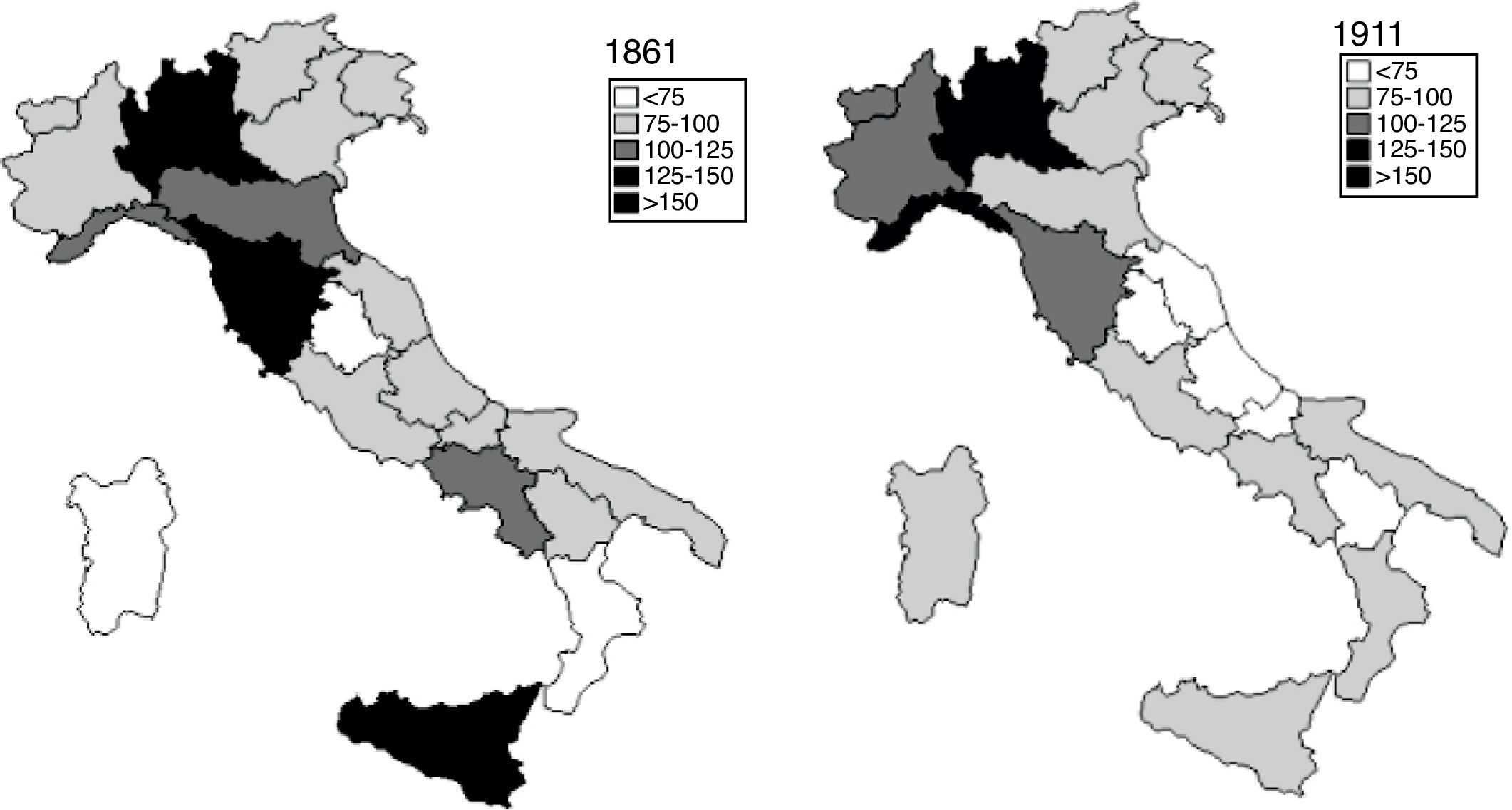
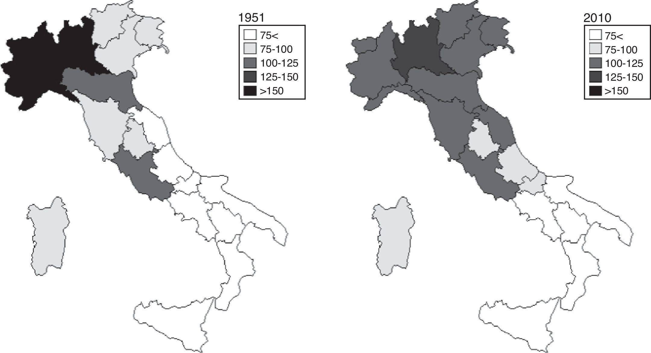
During the first phase of Italian industrialisation, the Southern regions lost ground in comparison with the Northern ones. In 1911, Campania was the only Southern region with a level of per capita GDP higher than the Italian average. During the first half of the last century, the North–South development gap widened continuously. In 1951, in all of the Southern regions, per capita income was below 75 percent of the Italian average. The regions of the “Industrial triangle” boasted considerably higher development levels than the rest of the country. A comparison between the years 1951 and 2010 (Fig. 5) shows an important change which finally came about during the last 60 years: both in the North and South some inner convergence occurred, while the North–South divergence continued to persist.
.")
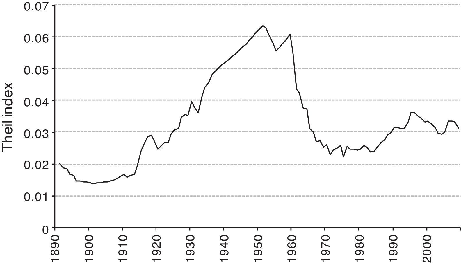
The Theil index can be usefully employed to highlight the trend of regional inequality in GDP during the last 120 years (Fig. 6). In 1891, the level of inequality was low. We see that it increased from the end of the Nineteenth century and reached its peak in the aftermath of World War 2, after a strong rise during the fascist period (1922–1943). In the 1950s, and particularly the 1960s, a sudden fall occurred. The existence of a remarkable regional convergence during the 1960s has been highlighted by different studies (Paci and Pigliaru, 1997; Terrasi, 1999). In particular, Terrasi (1999), examining the period 1950–1993, explicitly related regional convergence to national development, suggesting how the evolution of regional inequality partly followed a bell-shaped curve.

Disparity in regional GDP per capita measured through the Theil index 1891–2010.
From 1975 to 1980 onwards, inequality increased once more, although not dramatically. In the first decade of the new millennium Italian regional inequality was higher than in the 1970s, but only a little higher than it was at the start of Italian industrialisation.8 As J. Williamson stressed in 1965, regional inequality in Italy also followed an inverted U curve from modest pre-modern stability to a new stability, again on a modest level. The reason behind the inverted U curve of regional inequality is straightforward, when we look at the formula of the Theil index:
where Yi is GDP in region i, Y* is national GDP, Pi is the population of the region i and P* national population. Since Pi/P* is almost constant,9 when in a region the ratio Yi/Y* increases, inequality, represented by T, rises. Whenever, as a consequence of the start of modern growth, the same ratio Yi/Y* also increases in other regions, disparity grows. Finally, ever more widespread economic growth raises national GDP, Y*. The ratio Yi/Y* diminishes and approaches the percentage of national population (Pi/P). Consequently, inequality among regions diminishes.3Regional inequalities and industrialisation3.1A cross section analysis
The hypothesis we intend to test is that the particular evolution of Italian regional inequality could actually be linked to the regional spread of industry rather than the trend of national GDP. It is apparent that GDP levels, which are constantly on the rise during the epoch here under examination, cannot be easily correlated with regional disparities, initially rising, then diminishing and finally stabilising. A similarity exists, instead, with the concentration and spreading of industry. As far as we know this correlation has never been tested in literature on regional disparity in Italy.
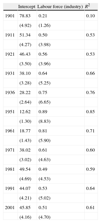
The existence of a correlation between the level of regional per capita GDP and the level of industrial labour force is confirmed by a cross section test where for all the census years, from 1901 until 2001, we regress GDP per head on industrial employment in each of our 16 regions through the following Eq. (3):
where the dependent variable y is per capita GDP in the region i divided by the national per capita GDP for each year, and the regressor is the percentage of labour force in industry out of the population of each region, divided by the same variable computed at national level.10 The results of cross section estimates for every decade from 1901 are shown in Table 3.
Regression results for census years 1901–2001.
| Intercept | Labour force (industry) | R2 | |
| 1901 | 78.83 | 0.21 | 0.10 |
| (4.92) | (1.26) | ||
| 1911 | 51.34 | 0.50 | 0.53 |
| (4.27) | (3.98) | ||
| 1921 | 46.43 | 0.56 | 0.53 |
| (3.50) | (3.96) | ||
| 1931 | 38.10 | 0.64 | 0.66 |
| (3.28) | (5.25) | ||
| 1936 | 28.22 | 0.75 | 0.76 |
| (2.64) | (6.65) | ||
| 1951 | 12.62 | 0.89 | 0.85 |
| (1.30) | (8.83) | ||
| 1961 | 18.77 | 0.81 | 0.71 |
| (1.43) | (5.90) | ||
| 1971 | 38.02 | 0.61 | 0.60 |
| (3.02) | (4.63) | ||
| 1981 | 49.54 | 0.49 | 0.59 |
| (4.69) | (4.53) | ||
| 1991 | 44.07 | 0.53 | 0.64 |
| (4.21) | (5.02) | ||
| 2001 | 45.85 | 0.51 | 0.61 |
| (4.16) | (4.70) |
Note: Ols estimates; heteroskedasticity robust standard errors t-stat in parentheses.
As might be expected, in 1901 there was no relation between regional GDP per capita and the industrial labour force participation rate: although the importance of industry was increasing, it was still poorly developed. From then on, however, with the progress of industrialisation, the relationship regional GDP/industrial labour force strengthened more and more, as the coefficients and the R2 reveal. A remarkable increase in the R2 had already occurred between 1901 and 1911. The correlation between regional GDP per head and regional industrial occupation became particularly high around 1951 and the effect of changes in the predictor on outcome, the coefficient β, more and more relevant; although even later on, the explanatory capacity of the predictor is highly significant. Considering the small number of observations per years, this exercise should only be seen as a preliminary step towards the panel estimates in the following section.
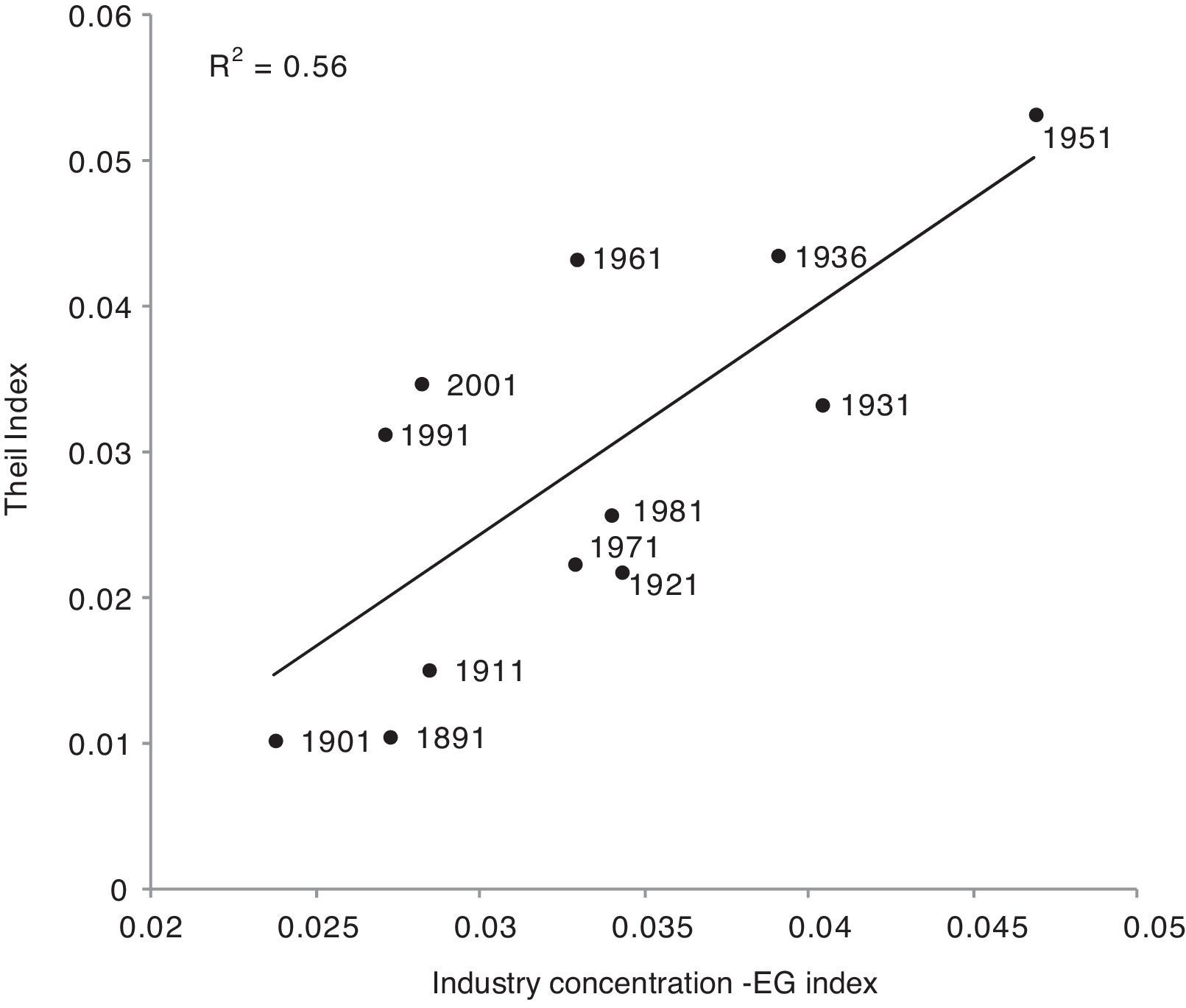
3.2Panel data analysisThe descriptive analysis presented in the previous sections, suggests how in Italy, just as in other countries, the evolution of regional disparities in income was closely related to the degree of industrial concentration. Schematically, from the end of the Nineteenth century to the early 1950s, industrial concentration increased while regions diverged; later, for approximately twenty years, industry spread and regions converged; finally, the degree of industrial concentration and the degree of inequality in income remained roughly stable. It is important to stress that our measure of regional inequality for both GDP and industrial labour force shows a bell-shaped curve when the independent variable is time. Since both curves describe a similar trend, their relationship is clearly linear. Fig. 7 illustrates the correlation existing between the Theil index of regional inequalities and the Ellison–Glaeser index of industrial concentration (as computed in Section 2) in the period 1901–2001. It is easy to see how the minimum values of the Ellison–Glaeser index and the Theil index are registered in 1891 and 1901, while their maximum values are seen in 1951. In the subsequent decades, both indexes diminish.

Data on regional labour force strongly limit the possibility to provide a more formal analysis of the relationship between regional inequality and industry concentration. The overall degree of concentration may, in fact, be computed only on a decadal basis (per census that is). Nevertheless, the relationship between regional disparities in GDP levels and the distribution of industry can be analysed through a different empirical strategy, a panel test, which allows us to exploit the longitudinal dimension of our dataset that contains observations for 16 regions over 11 periods both for GDP per capita and labour force.
To test this relationship we estimated the following equation:
in which the dependent variable (disparity in GDP per capita) is computed as:where DY is a measure of inequality in GDP per region; Yi is GDP of the region i, Y* is national GDP, Pi is the population of each region i and P* is the national population. The independent variable, that is regional inequality in industrial labour force, is similarly computed as:where DL is the measure of inequality in the industrial labour force Li in the region i and L* is the national labour force in industry.
The idea behind this calculation is the same as that of the Theil index, which is computed as the sum of the specific inequalities per region calculated through the previous two Eqs. (5) and (6). Both DY and DL measure the discrepancy between the distribution of a character (GDP per capita and labour force in industry in our case) and the distribution of the population in a region. When this ratio is 1 for a region, then this group's contribution to inequality is zero. Both equations measure how far a particular region i is from perfect equality.
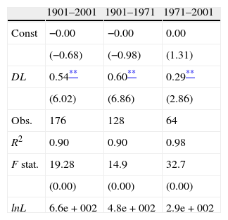
The results of fixed effect estimates, reported in Table 4, confirm the existence of a robust relationship between regional GDP and regional industrial labour force both over the whole period under examination and in two sub-periods 1901–1971 and 1971–2001.11
Results of fixed effect estimates, 1901–2011.
| 1901–2001 | 1901–1971 | 1971–2001 | |
| Const | −0.00 | −0.00 | 0.00 |
| (−0.68) | (−0.98) | (1.31) | |
| DL | 0.54** | 0.60** | 0.29** |
| (6.02) | (6.86) | (2.86) | |
| Obs. | 176 | 128 | 64 |
| R2 | 0.90 | 0.90 | 0.98 |
| F stat. | 19.28 | 14.9 | 32.7 |
| (0.00) | (0.00) | (0.00) | |
| lnL | 6.6e+002 | 4.8e+002 | 2.9e+002 |
Note: the dependent variable is DY. Fixed effects estimates – t-statistics in parentheses.
We could question whether a unique independent variable is enough to capture a complex phenomenon, such as the trend of regional inequality during the phase of modern growth. DL actually captures several effects, such as the shift of the labour force from agriculture, the high rate of increase in the productive capacity of the economic system, the rising levels of per capita GDP and labour productivity per region. Despite its limitations, the analysis indicates how the relative degree of regional development is strictly related to the degree of relative industrialisation and this, consequently, determines the overall degree of inequality.
4The North–South divide4.1The origins and development of Italian dualismThe results of our calculations seem to be quite reassuring. Regional inequalities in both per capita GDP and structure of the labour force were once low, later to increase but finally to fall again. In 2000–2003, the degree of regional disparity was lower in Italy than in Belgium and similar to that in France and Spain (Ezcurra and Rapún, 2006). However, the history of the North and South seems to suggest a quite diverse evolution. If the disparity between the North and the South is still remarkable in 2011 and in the South per capita product is 58 percent of that of the North (Section 2), how can we reconcile this modest level of regional disparities with the high divide between these two Italian areas?
Historians have emphasised the existence, already in 1861, of North–South differences rooted in diverse historical evolutions. From differences in social indicators, Eckaus (1961) estimated a disparity of 15–25 percent in the average income between North and South immediately after the Unification. Pescosolido (1998) proposed a North–South disparity in 1861 in the order of 10 percent. Esposto (1997) maintained that in 1871 per capita GDP in the South was 13 percent lower than the national average, while, according to Brunetti et al. (2011) the North–South difference in per capita GDP was 15 percent, at the same date.12 These authors do not actually refer to regional disparity, but to the divide between North and South. Despite the uncertainties on regional differences in GDP per head, before 1891, all of these scholars agree on their modest degree and on the upward trend some decades after the Unification of the country.
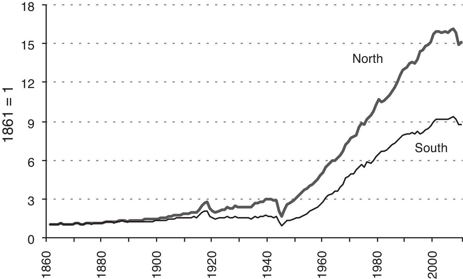
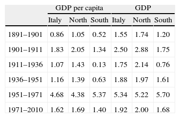
The available time series show that a remarkable divergence began at the start of modern growth in Italy and is clearly tested by data both on the rate of increase (Table 5) and on the level of GDP (Fig. 8). It may be noted that, before 1901, per capita growth was weak. In the first decade of the Twentieth century growth accelerates, but the growth rates in the Southern regions are lower than in the North. Only in the period 1951–1971 are growth rates higher in the South than in the rest of the country: a weak phase of convergence occurs.
Yearly rates of GDP growth in the North, the South and Italy 1891–2010 (%).
| GDP per capita | GDP | |||||
| Italy | North | South | Italy | North | South | |
| 1891–1901 | 0.86 | 1.05 | 0.52 | 1.55 | 1.74 | 1.20 |
| 1901–1911 | 1.83 | 2.05 | 1.34 | 2.50 | 2.88 | 1.75 |
| 1911–1936 | 1.07 | 1.43 | 0.13 | 1.75 | 2.14 | 0.76 |
| 1936–1951 | 1.16 | 1.39 | 0.63 | 1.88 | 1.97 | 1.61 |
| 1951–1971 | 4.68 | 4.38 | 5.37 | 5.34 | 5.22 | 5.70 |
| 1971–2010 | 1.62 | 1.69 | 1.40 | 1.92 | 2.00 | 1.68 |
.")
Per capita GDP in the North and the South 1861–2010 (1861=1).
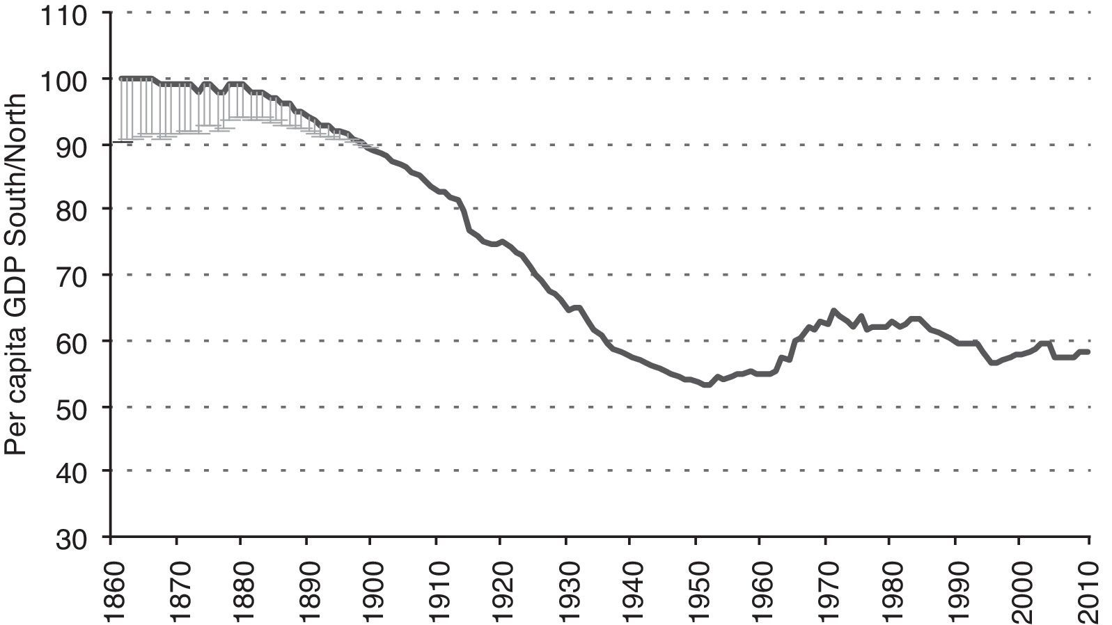
The North–South inequality is more apparent whenever we measure the North–South differential, dividing per capita GDP in the South by that in the North. We lack reliable figures on North–South inequality before 1891. On the eve of World War 1, the South–North ratio in product per capita was 80 percent; in 1951 it was 50 percent (Fig. 9). At that time, all of the Southern regions shared a level of per capita GDP lower than the national average. The two and a half decades after the war was the only period when GDP rose faster in the South than in the North. However, after 25 years of modest progress, per capita GDP in the South began to fall again relative to that in the North and then stabilised around 60 percent.
.")
Ratio between per capita GDP in the South and the North 1861–2010 (%).
Since both data on regional disparity and North–South inequality seem to be reliable, the only explanation for the diverse evolution of disparities among regions and between North and South is that inequality, once widespread across the national territory, depended ultimately on the divergence between two parts of the same country which were internally relatively homogeneous. We could thus hypothesise a rising convergence within both the North and South together with a rising divergence between these two sections. We present two different and complementary statistical methods aimed at specifying this reshaping of the Italian economic geography.
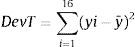
4.2Dualism and disparities: a first calculationA first method in order to distinguish dualism and disparities is that of exploiting a property of the deviance: having a set divided into two subsets, total deviance (DevT) is equal to the sum of the deviances within the subsets (DevW) plus the deviance between the averages of the subsets (DevB). That is:
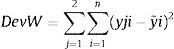
DevT represents total deviance in per capita product among our 16 regions:where yi is per capita GDP of the region i, and y¯ the average per capita GDP of all the regions, that is national per capita GDP. Deviance within the subsets North and South (DevW) is represented by:
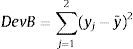
The deviance between the two groups of regions, North and South (DevB), is equal to:
The share of North–South disparity (Dns) of total regional disparity is then computed as:

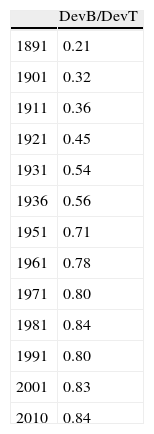
Table 6 reports the ratio between the North–South deviance and total deviance among regions according to Eq. (11). We see how the North–South disparity only accounted for 21 percent of total regional disparity in 1891. At that time, the North and South were hardly distinguishable. However, it can be seen that, in the following century, the North and South gradually became two different economies. From the 1970s onwards, DevB accounted for 80 percent of the total deviance (DevT). While convergence occurred both within the North and the South (and DevW declined), divergence widened between the North on the one hand and the South on the other (and then DevB).
Ratio of the deviance between the North and South (DevB) and total deviance (DevT) 1891–2010.
| DevB/DevT | |
| 1891 | 0.21 |
| 1901 | 0.32 |
| 1911 | 0.36 |
| 1921 | 0.45 |
| 1931 | 0.54 |
| 1936 | 0.56 |
| 1951 | 0.71 |
| 1961 | 0.78 |
| 1971 | 0.80 |
| 1981 | 0.84 |
| 1991 | 0.80 |
| 2001 | 0.83 |
| 2010 | 0.84 |
The conclusion is that convergence occurred over the period both within the North and the South, but North–South divergence rose.
4.3Dualism and disparities: a second calculationA graphic presentation of the North–South disparity within the Italian regional disparity can be reached by computing the Theil index of the North–South divide and by comparing it to the national Theil index. The Theil index for inequality between North and South is computed using the following formula (12):
where DNS is the North–South divide and Yj and Pj per capita GDP in each area and population in each area, divided by national GDP (Y*) and national population (P*).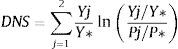
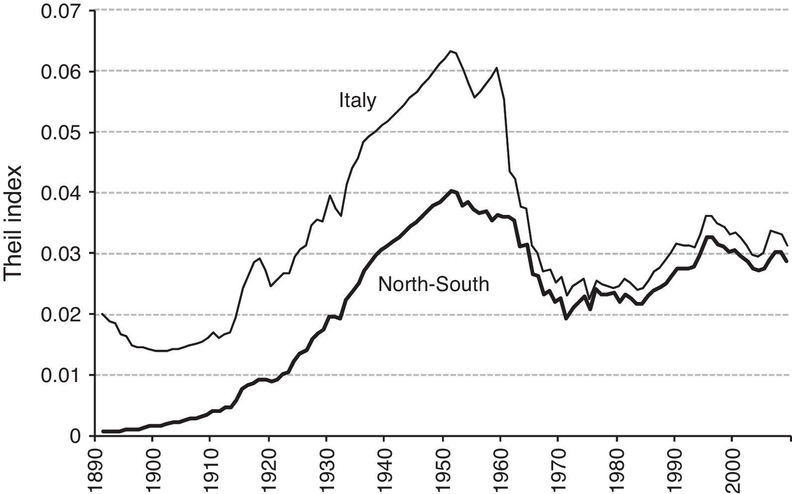
In Fig. 10, the Theil indices for the whole of Italy and the North and South are compared. We see that, at the beginning, the North–South disparity was negligible, but increasing. The analysis of the deviance is confirmed. The decline in the level of regional inequality from 1950 cancelled the disparities among the regions in both the North and South, but hardly interested the inequality between North and South. Gradually Italian regional inequality intensified between North and South, with the formation of two convergence clubs: a rich one including most of the Centre and North, and a poor one consisting of a small group of Southern regions (Paci and Pigliaru, 1999).

Theil indices between the regions and between North and South 1980–2010.
In order to explain regional disparity, and especially the North–South divide, several scholars recall remote causes: the different history of the North and South in the distant past (Guiso et al., 2008) or during the Middle Ages (Putnam, 1993), or even supposed genetic differences in the intelligence quotients between the Southern and Northern populations (Lynn, 2010). A traditional approach in Italy is to see the North–South divide as the consequence of political errors and then to attribute it to faults by governments and mistaken economic policies.
In this contribution we have investigated the proximate causes and focused on measurable facts. These alleged social and political causes, both distant and recent, are often impossible to plausibly measure. They are frequently object for conjecture and political debates and are out of our perspective. In our view, to be properly understood, regional inequality must be set within the general process of modern growth and can be realistically linked to the structural change which has taken place in Italy over the last 150 years. We have examined this process, focusing on the relationship between the geographical distribution of industry and the evolution of regional inequality.
The evolution of regional inequalities in Italy in part confirms Williamson's hypothesis: a long phase of divergence started with the process of industrialisation, when industrial concentration increased; later, however, the spreading of industry engendered a relative convergence. Different is the pattern of inequality in per capita GDP between North and South. In this case, we do not find any bell-shaped curve: per capita income levels diverged in a first long-phase of about 60-years (1891–1951), slightly converged in a second short period of about 20-years (1955–1975), and remained roughly stable in the subsequent period as they are today.
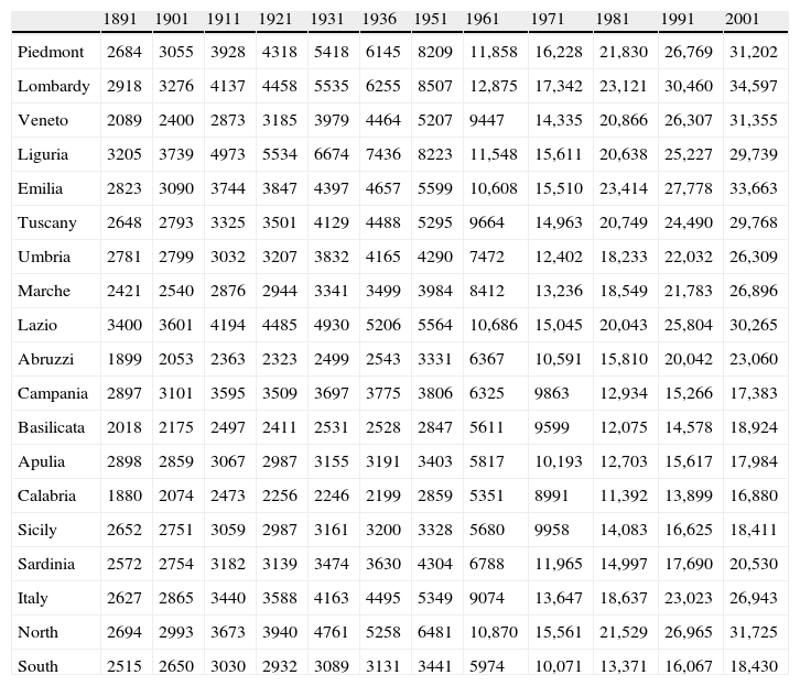
Sources of the Italian GDP series are presented in Daniele and Malanima (2011). The series of regional GDP in 1891, 1911, 1938 in Table A.2 have been worked out from the following sources: agriculture (Federico, 2003a, 2003b); industry (Fenoaltea, 2003b); services (Felice, 2005a, 2005b). Series for the years comprised between the benchmarks have been calculated interpolating regional disparities in per capita GDP (with respect to the index Italy=1). This interpolation method permits the obtaining of yearly data for the periods comprised between the benchmarks (e.g. data used for Figs. 6, 8 and 9). It is easy to see how this method gives regional GDP per capita estimates whose trends, between the benchmark years, replicate exactly the national business cycle. A serious limitation does not emerge in absence of severe and regional specific supply-side shocks (such as natural catastrophes or profound deindustrialisation). In order to test our procedure, we applied the same method to Istat regional data for the period 1980–2004 (more or less the same number of years as our reconstruction between the benchmarks for the years 1891–1951); we predicted, that is, regional per capita GDP in 1980–2004 with the same method we utilised for the earlier periods. The partial correlations between predicted and actual GDP per capita for the cross-sections were, for the years 1980–2004, in the order of 0.99. The result of this test supports our previous reconstructions of annual regional data from benchmark years. For 1951–1959 we utilised data on gross product from Svimez (1961). For the years 1963–69, we took data from Unioncamere (1972). For 1970–1979: Svimez (1993). For the three decades 1980–2009: Istat, Conti economici regionali. The differentials of our previous Table 2 have been obtained by dividing per capita regional output by the national per capita output. We did the same in Table 2, for the North and the South. Data on regional GDP have been presented and discussed in Daniele and Malanima (2007, 2011) (Table A.1).
Regional per capita GDP 1891–2001 (euros 2010).
| 1891 | 1901 | 1911 | 1921 | 1931 | 1936 | 1951 | 1961 | 1971 | 1981 | 1991 | 2001 | |
| Piedmont | 2684 | 3055 | 3928 | 4318 | 5418 | 6145 | 8209 | 11,858 | 16,228 | 21,830 | 26,769 | 31,202 |
| Lombardy | 2918 | 3276 | 4137 | 4458 | 5535 | 6255 | 8507 | 12,875 | 17,342 | 23,121 | 30,460 | 34,597 |
| Veneto | 2089 | 2400 | 2873 | 3185 | 3979 | 4464 | 5207 | 9447 | 14,335 | 20,866 | 26,307 | 31,355 |
| Liguria | 3205 | 3739 | 4973 | 5534 | 6674 | 7436 | 8223 | 11,548 | 15,611 | 20,638 | 25,227 | 29,739 |
| Emilia | 2823 | 3090 | 3744 | 3847 | 4397 | 4657 | 5599 | 10,608 | 15,510 | 23,414 | 27,778 | 33,663 |
| Tuscany | 2648 | 2793 | 3325 | 3501 | 4129 | 4488 | 5295 | 9664 | 14,963 | 20,749 | 24,490 | 29,768 |
| Umbria | 2781 | 2799 | 3032 | 3207 | 3832 | 4165 | 4290 | 7472 | 12,402 | 18,233 | 22,032 | 26,309 |
| Marche | 2421 | 2540 | 2876 | 2944 | 3341 | 3499 | 3984 | 8412 | 13,236 | 18,549 | 21,783 | 26,896 |
| Lazio | 3400 | 3601 | 4194 | 4485 | 4930 | 5206 | 5564 | 10,686 | 15,045 | 20,043 | 25,804 | 30,265 |
| Abruzzi | 1899 | 2053 | 2363 | 2323 | 2499 | 2543 | 3331 | 6367 | 10,591 | 15,810 | 20,042 | 23,060 |
| Campania | 2897 | 3101 | 3595 | 3509 | 3697 | 3775 | 3806 | 6325 | 9863 | 12,934 | 15,266 | 17,383 |
| Basilicata | 2018 | 2175 | 2497 | 2411 | 2531 | 2528 | 2847 | 5611 | 9599 | 12,075 | 14,578 | 18,924 |
| Apulia | 2898 | 2859 | 3067 | 2987 | 3155 | 3191 | 3403 | 5817 | 10,193 | 12,703 | 15,617 | 17,984 |
| Calabria | 1880 | 2074 | 2473 | 2256 | 2246 | 2199 | 2859 | 5351 | 8991 | 11,392 | 13,899 | 16,880 |
| Sicily | 2652 | 2751 | 3059 | 2987 | 3161 | 3200 | 3328 | 5680 | 9958 | 14,083 | 16,625 | 18,411 |
| Sardinia | 2572 | 2754 | 3182 | 3139 | 3474 | 3630 | 4304 | 6788 | 11,965 | 14,997 | 17,690 | 20,530 |
| Italy | 2627 | 2865 | 3440 | 3588 | 4163 | 4495 | 5349 | 9074 | 13,647 | 18,637 | 23,023 | 26,943 |
| North | 2694 | 2993 | 3673 | 3940 | 4761 | 5258 | 6481 | 10,870 | 15,561 | 21,529 | 26,965 | 31,725 |
| South | 2515 | 2650 | 3030 | 2932 | 3089 | 3131 | 3441 | 5974 | 10,071 | 13,371 | 16,067 | 18,430 |
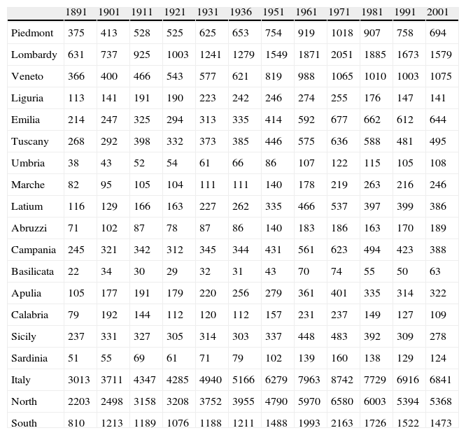
Labour force in the secondary sector 1891–2001 (000).
| 1891 | 1901 | 1911 | 1921 | 1931 | 1936 | 1951 | 1961 | 1971 | 1981 | 1991 | 2001 | |
| Piedmont | 375 | 413 | 528 | 525 | 625 | 653 | 754 | 919 | 1018 | 907 | 758 | 694 |
| Lombardy | 631 | 737 | 925 | 1003 | 1241 | 1279 | 1549 | 1871 | 2051 | 1885 | 1673 | 1579 |
| Veneto | 366 | 400 | 466 | 543 | 577 | 621 | 819 | 988 | 1065 | 1010 | 1003 | 1075 |
| Liguria | 113 | 141 | 191 | 190 | 223 | 242 | 246 | 274 | 255 | 176 | 147 | 141 |
| Emilia | 214 | 247 | 325 | 294 | 313 | 335 | 414 | 592 | 677 | 662 | 612 | 644 |
| Tuscany | 268 | 292 | 398 | 332 | 373 | 385 | 446 | 575 | 636 | 588 | 481 | 495 |
| Umbria | 38 | 43 | 52 | 54 | 61 | 66 | 86 | 107 | 122 | 115 | 105 | 108 |
| Marche | 82 | 95 | 105 | 104 | 111 | 111 | 140 | 178 | 219 | 263 | 216 | 246 |
| Latium | 116 | 129 | 166 | 163 | 227 | 262 | 335 | 466 | 537 | 397 | 399 | 386 |
| Abruzzi | 71 | 102 | 87 | 78 | 87 | 86 | 140 | 183 | 186 | 163 | 170 | 189 |
| Campania | 245 | 321 | 342 | 312 | 345 | 344 | 431 | 561 | 623 | 494 | 423 | 388 |
| Basilicata | 22 | 34 | 30 | 29 | 32 | 31 | 43 | 70 | 74 | 55 | 50 | 63 |
| Apulia | 105 | 177 | 191 | 179 | 220 | 256 | 279 | 361 | 401 | 335 | 314 | 322 |
| Calabria | 79 | 192 | 144 | 112 | 120 | 112 | 157 | 231 | 237 | 149 | 127 | 109 |
| Sicily | 237 | 331 | 327 | 305 | 314 | 303 | 337 | 448 | 483 | 392 | 309 | 278 |
| Sardinia | 51 | 55 | 69 | 61 | 71 | 79 | 102 | 139 | 160 | 138 | 129 | 124 |
| Italy | 3013 | 3711 | 4347 | 4285 | 4940 | 5166 | 6279 | 7963 | 8742 | 7729 | 6916 | 6841 |
| North | 2203 | 2498 | 3158 | 3208 | 3752 | 3955 | 4790 | 5970 | 6580 | 6003 | 5394 | 5368 |
| South | 810 | 1213 | 1189 | 1076 | 1188 | 1211 | 1488 | 1993 | 2163 | 1726 | 1522 | 1473 |
Regional labour forces data have been calculated within the International Network for the Comparative History of Occupational Structure (INCHOS), coordinated by O. Saito (Hitotsubashi University) and L. Shaw-Taylor (Cambridge Group for the History of Population and Social Structure). Many more details on labour force are presented in Daniele and Malanima (forthcoming). See also the important article by Zamagni (1987). Data between 1881 and 1961 are from Vitali (1970). Data from 1971 are from Istat series of population censuses and data on labour force.
. Piemonte includes Aosta Valley, Veneto includes Friuli Venezia Giulia and Trentino Alto Adige; Abruzzi and Molise are also combined into a single region.")
Map of the Italian regions. Note: actually, in 2010, the Italian Regions are 20. This Map and our Maps 1–8 refer to 16 homogeneous regions. Some of them are sets of regions existing nowadays (and then it is easy to aggregate figures referring to them into bigger sets). Piemonte includes Aosta Valley, Veneto includes Friuli Venezia Giulia and Trentino Alto Adige; Abruzzi and Molise are also combined into a single region.
Estimates of regional GDP have been published by Felice (2007) and Brunetti et al. (2011). Felice (2011) reached results similar to ours. Since his reconstruction is not based on present, but on past regional borders, his results are hard to exploit and relate to other regional indicators.
With the exception of 1891, when the population census was not held. For 1891, our data in Table 1 are based on the interpolation through the censuses held in 1881 and 1901.
We refer here to the share of labour force in industry out of the total population and not to the participation rate. Data in Table 1 refer to the participation rate (the ratio of workers in industry to the total labour force).
The interactions between potential market size, transport costs and economies of scale in determining the location of industry are at the centre of the new economic geography; see, for example, Krugman (1991a, 1991b).
As will be shown in Section 3.
In our regional series and in the following pages we use the series of Italian GDP presented in Daniele and Malanima (2011, App. 1). In this same App. 1, we discuss the differences between this series and that by Baffigi (2013) – the series by Baffigi have already been presented in Baffigi (2011) and Vecchi (2011, p. 427). The correlation between our series and those by Baffigi is 0.999. Using the series by Baffigi, our following analysis would be totally unaffected.
Looking at the disparities between the East and West of the Apennines, Sicily and Sardinia are not included.
Here we refer to regional disparity and not North-South disparity, still significant and stable at a high level.
Some changes did in fact occur in the relative demographic weight of specific regions, although these changes were on the whole modest. In the Southern regions the high rate of emigration was, in fact, counterbalanced by a high birth rate. See, on the matter, the still useful articles by Di Comite and Imbriani (1982) and Di Comite (1983).
In this case, we computed the industrial participation rate as the industrial labour force in each region divided by the population of the same region, in order to capture the abandonment of the labour market by a share of the industrial labour force. This abandonment is captured if the denominator of our ratio is population whereas it is not if the denominator is labour force.
The year 1971 has been chosen since from the early Seventies onwards the North-South divide is more or less stable.
Brunetti et al. (2011, pp. 220–222, 234, 428) do not specify how they reached their results. There is no reference at all to the sources, and especially to the kind of wages used in their estimation: agricultural or industrial? How much data? To what regions do these data refer? The lack of clarity on the procedure does not allow us to exploit their calculations. Felice and Vasta (2012) estimated for 1871 a North-South disparity of 8.7 percent (per capita GDP in the South is 91.3 percent that of the North), on the basis of real GDP in PPP 2008 US dollars.