


The economic recession in the European countries during the current financial crisis and the widespread worsening of the financial situation have resulted in wide macroeconomic differences across countries. In this paper we use the method of self-organizing maps (SOM) to compare the macroeconomic financial imbalances among European countries. We detect different profiles of countries and identify the public expenditure and the saving rate as the most critical variables that impacts on the national financial situation. In addition, since several countries of the European Union have regions with some degree of economic and financial competences, we study the influence of the regions on the whole country. Thus, we classify and compare the Spanish and German regions and we prove the impact of the regional situation on the whole country situation.
The current financial crisis, although initially a bank-level crisis, has resulted in a situation of generalized illiquidity in financial markets and financial instability. Whereas in the first months the crisis had a microeconomic impact over the firms and the financial intermediaries, it later reached macroeconomic dimensions and the solvency of some countries became under discussion.
The switch from microeconomic financial distress to macroeconomic distress can be verified from 2010 in after. At the beginning of 2010, the European Union (EU), the International Monetary Fund (IMF) and the European Central Bank (ECB) granted 110 billion of euros credit to Greece given the inability of this country to serve its public debt. Some days later, a permanent fund for ransom of 750 billion was created due to the threat of international contagion and in order to reinforce the international reliability of the European currency. Some months later, in November 2010, Ireland received 87 billion of euros as financial help to refinance the public debt. In April 2011, Portugal asked and received from the EU and the IMF financial help amounting to 78 billion of euros. In addition, the implausibility of Greece to serve the interest of the public debt after the first bailout casted new doubts about the stability of the euro area after May 2011. From April 2012, the main European concern has focused on Spain, which has received 100 billion of euros credit line from the EU.1 More recently, in March 2013, a 10 billion of euros bailout was announced for Cyprus.
In a financial environment so globalized as the current one, the national financial distresses can be transmitted to other countries, be a threat for the global economic recovery and lead to a generalized collapse of the credit flow to the real economy. In spite of the fact that in July 2011 the European Banking Authority (EBA) published the results of the stress tests of the financial institutions2 with an acceptable result in general terms, financial markets did not rely completely on the States and Governments. In fact, the credit rating of the United States and of many European countries worsened in the summer of 2011.
An implication of these facts is that Europe should have some tools to assure the effective comparability among countries as a means to assure the efficiency of the correctional policies. In addition, early warning systems in the European financial system could alleviate the asymmetric impact of the financial crisis among countries and avoid the threat of “two speed Europe” that could put in danger the common currency.
The model we propose is a step forward to have such a tool for the detection and management of divergences among countries to anticipate this danger. The analysis within countries can also provide interesting insights since the regions or the states with economic autonomy can contribute significantly to the (in)stability and growth of the whole country. The earlier the economic unbalances among regions are detected, the easier they could be corrected.
Spain is an interesting case to test our model given the financial problems that it is going through, and the special regional configuration of the Public Administration. The Spanish regional governments (Autonomous Communities or AA.CC. hereinafter) have high levels of financial leverage that cast doubts on the ability of Spain to meet its financial engagements. This is the view of the rating agencies, which have systematically downgraded the credit rating of the AA.CC., and the view of the EU, which has required the Spanish Government to control the financial deficit of the AA.CC. In order to enable the comparability of our model, we apply our model to Germany. Although the German states (Bundesländer) are considered NUTS-1 and the Spanish AA.CC. are considered NUTS-2 according to the European classification,3 both kinds of institutions are comparable in terms of political and economic competences. In addition, the quite different financial situation of Germany and Spain allows us to test the “virtuous or vicious circle” effect of regions on the country as a whole.
Our paper aims to contribute to the literature on national financial balance providing a complete and simple model. Most of the international comparisons until now have been based on one single indicator, which results in the loss of explanatory ability. Our model is self-organizing maps (SOM), a technique based on neural networks (NN) that enables complex international classifications by combining several variables.
Although NN have been widely used in business and finance domains, the analysis of country financial issues is a relatively unexplored field and has promising avenues for research (Herrero et al., 2011; Yim and Mitchell, 2005). The SOM method has been previously used to classify regions (Alfaro Cortés et al., 2003). These authors show the validity of the SOM method for the socio-economic classification of the European NUTS-2 regions. Unlike these authors’ research, which focuses on social issues, our paper is concerned with financial and economic factors.
Our objective is twofold. First, we use the SOM method to perform a classification of the European countries depending on their solvency using the most common variables in the literature. The identification of the similarities and differences among countries is relevant information to detect imbalances in order to take correcting measures to avoid the propagation of financial crises. Our second aim is to relate the financial situation of the country as a whole with the financial situation of its regions. Recent concerns about the impact of the financial situation of the regions on the solvency of the whole country advice for a more in-depth analysis. Accordingly, we perform a classification analysis of the German and Spanish regions. Germany and Spain are two countries with an analogous territorial organization but with diametrically different financial situation, so that our analysis can cast some light on to which extent the national distress is due to the regional macroeconomic imbalance.
Our paper is divided into six sections. After the introduction, in the second Section we present the foundations of the neural networks as methods for financial analysis and prediction; we also describe the SOM methodology. In Section 3 we apply our model to the European countries in order to have an international classification and to identify the most determinant variables of the financial situation. We compare our results with the ones from previously used techniques as the K-means and the Factor/K-means clustering procedures In Sections 4 and 5 we reply an analogous analysis for the Spanish AA.CC. and the German Länder. In Section 6 we conclude with the most remarkable ideas and we point out some applications of our model for the design of economic policies.
2The neural network method2.1Foundations of neural networks in business and financeNN are one the most widely used models among the intelligence techniques. They have mathematical and algorithmic elements that mimic the biological neural networks of the human nervous system, so that they have similarities with the functioning of the human brain (Kohonen, 1993). NN take into account the relations among different groups of artificial neurons and processes the information about them using a so-called connectionist approach, in which network units are connected by a flow of information.
Neural networks are a powerful set of algorithms whose objective is to find a pattern of behavior (Moreno and Olmeda, 2007) and that have two main advantages compared to more traditional multivariate statistical techniques. First, NN do not require any kind of assumption about the statistical distribution of the data. Second, NN are not limited by linear specifications as many of the traditional techniques are. So, a successful NN implementation generates a system of relationships that has been learnt from observing past examples and is able to generalize these lessons to new examples.
As shown by Vellido et al. (1999) and Wong and Selvi (1998), NN have been profusely used in several domains of business, management, marketing and production. These applications usually involve the interaction of many diverse variables that are highly correlated, frequently assumed to be nonlinear, unclearly related, and too complex to be described by a mathematical model.
The use of neural networks in finance applications has been previously investigated in a number of areas such as loan segmentation, country investment risk, forecasting market movement, and credit scoring (Baesens et al., 2005; Becerra-Fernandez et al., 2002; Falavigna, 2012; Huang et al., 2005). NN have been used even in accounting issues to examine the occurrence of earnings management in various contexts (Höglund, 2012). By far, the main application of NN is bankruptcy and insolvency prediction, which accounts for around 30% of contributions (Vellido et al., 1999).
The general outcome of such works is that in the credit industry, neural networks have been considered to be accurate tool for credit analysis (Min and Lee, 2008). Similarly, Guresen et al. (2011) show that in most of the cases NN models give better result than other methods in forecasting stock markets movements.
Dutta and Shekhar (1988) pioneered the use of NN for corporate bond ratings. According to their results, the predictive success rate of NN was 88.3% compared to 64.7% for the regression model. Such significant results motivated further implementations of NN for bond ratings. Surkan and Singleton (1990) compare the NN against the multivariate discriminant analysis and find that the former perform significantly better. Kim et al. (1993), Lee and Choi (2013) and Maher and Sen (1997) also compare the performance of the regression analysis, the multivariate discriminant analysis, the logistic regression and the rule-based methods with NN for the classification of debt ratings. In all the cases the highest percentage of correctly classified bonds was achieved with NN. Likewise, Ravi Kumar and Ravi (2007) comprehensively review the methods developed to predict bank failures and conclude that the traditional statistical techniques are all outperformed by the NN. The results of Mokhatab Rafiei et al. (2011) also show that NN models achieved 98.6% accuracy rates in predicting financial health of Iranian companies, whereas multiple discriminant analysis reached 80.6%.
In the international arena Nag and Mitra (1999) rely on NN to predict some Far East currency crises, and Franck and Schmied (2003) improve the prediction of the currency crisis contagion by using NN. Interestingly, Bennell et al. (2006) use a 70 countries sample to demonstrate that NN represent a superior technology for calibrating and predicting sovereign ratings relative to the ordered probit modeling, which had been considered until recently the most successful approach (Trevino and Thomas, 2001).
As a possible explanation of all these results, Brockett et al. (1994) and Wong and Selvi (1998) suggest that NN have lower-prediction risk and less variance in their errors than the other statistical techniques because they not only accumulate and recognize patters of knowledge based on experience, but also constantly adapt to new environmental situations by permanent retraining and relearning. Kim and Kang (2010) and Shin and Lee (2002) underline the widespread use of NN as an alternative methodology for bankruptcy prediction and show that the artificial intelligence techniques are less vulnerable to the restrictive assumptions on data than the conventional statistical methods. These arguments are consistent with Fioramanti (2008), who focuses on the recent financial crisis. As stated by this author, the indicators of debt, currency crises, and systemic crises are non-linearly related. Since NN are non-parametric models that allow the violation of the rigid assumptions on the data distribution, NN have a say in predicting the contagion of the financial crisis episodes.
Despite these facts, to be honest one has to acknowledge that NN should not be viewed as a panacea, since they also presents various weaknesses. They are like black boxes and one can never know their internal working. In addition, NN are a family of models with many members to choose from. Thus, NN can be ad hoc tailored, so that the results could be affected by the design of the net. Likewise, a design good for solving one problem might not be as good for solving some other problem. As Gonzalez (2000) suggests, NN should be considered as a powerful complement to standard econometric methods, rather than a substitute.
2.2The self-organizing maps (SOM)There are two types of neural networks: the supervised and the non-supervised networks. The supervised networks require the definition of a set of input and output data, so that the network progressively adjusts the results to the expected output. The non-supervised networks are especially suited for exploratory analyses and are a suitable method for data clustering and efficient grouping.
In this latest kind of networks, neurons learn in an unsupervised way since there is not an objective output that the network has to provide. Consequently, there is not a pattern to let the network know whether it works properly. Thus, the network has to discover on its own the common patterns among the inputs. Therefore, the neurons have to self-organize conditional on the data from outside.
Non-supervised networks can be classified into two types: non-competitive and competitive networks. In the competitive networks, nodes compete for the right respond to a subset of the input data. The aim of this training is that, facing an input pattern, only one neuron (or a node of neurons) is activated. The other neurons are annulled. The result of this process is the network classifying the inputs into different homogeneous clusters. One of the best examples of competitive networks is the SOM, which has been used to predict currency crises and debt crises (Arciniegas Rueda and Arciniegas, 2009).
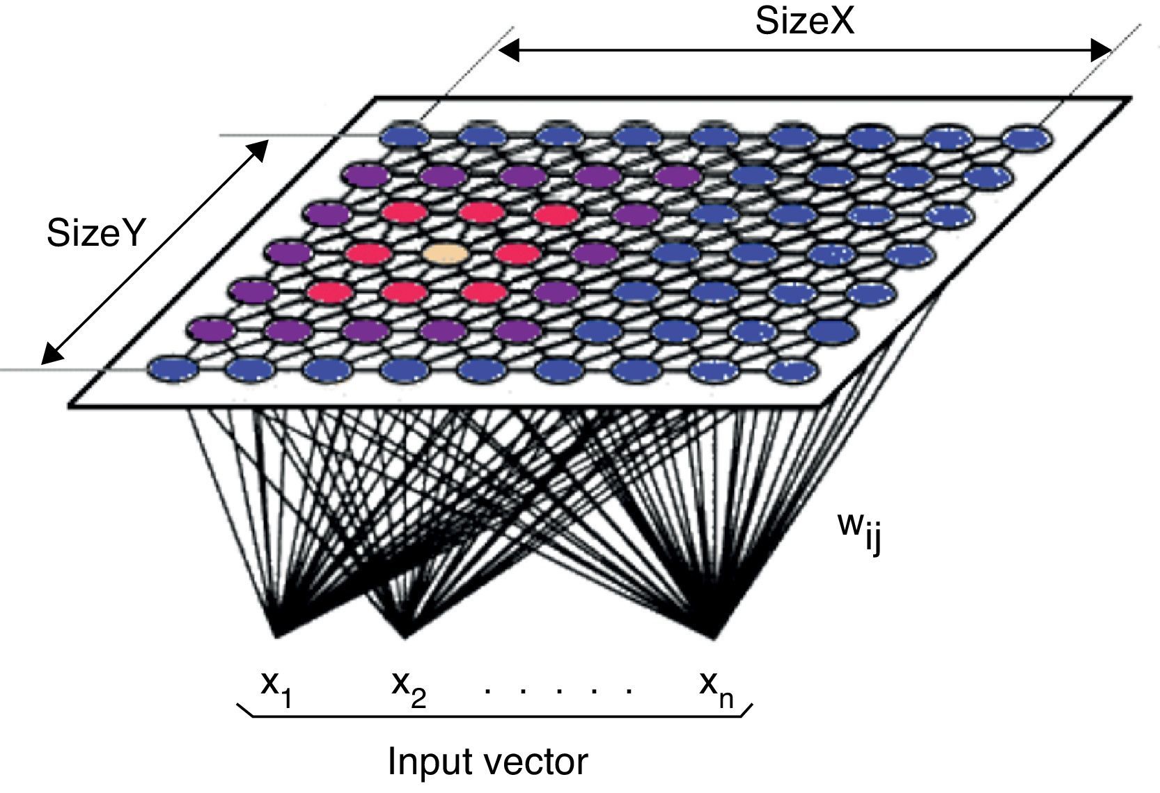
As shown in Fig. 1, in the SOM the neurons of the input layer are connected with all the neurons of the output layer through synaptic weights. Consequently, the information provided by each neuron of the input layer is transmitted to all the neurons of the output layer. All the neurons of the output layer receive the same set of inputs from the input layer.

The objective of a competitive network is to find the neuron of the output layer with the most similar synaptic weights to the values of the input layer neurons. To do so, each neuron calculates the difference between the input pattern and the set of synaptic weights of each output neuron. Conditional upon this calculation, the winning neuron is the one with the least difference or the shortest Euclidean distance between its weights and the set of inputs. The Euclidean distance is not the only measure to calculate the distance, but it is the most metric.
The distance between the neurons of the output layer and the vector of input patterns is calculated according to this equation:
where Xk is the input of the k-input neuron and di,j,(t) is the Euclidean distance of the (i,j) neuron in t relative to the input pattern for a network with i×j neurons in the output layer and k neurons in the input layer. The winning neuron is the one with the shortest Euclidean distance computed as: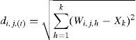
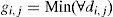
After determining the winning neuron, all the neurons in the network receive an output equal to zero but the winning neuron receives an output equal to one. Later, the weights of the winning neuron are adjusted with a learning rule to proxy these weights to the input pattern that has made the neuron win. In this way, the neuron whose weights are the closest ones to the input pattern is updated to become even closer. The result is that the winning neuron has more chances to win the competition in the next data entry for a similar input vector and has fewer chances for the competition if the input vector is different. It means that the neuron has specialized in this input pattern.
The equation that proxies the weights of the wining neuron and of the neighborhood function neurons is the next one, where α is the learning ratio, Xk(t) is the input pattern in t and Wjik(t) is the synaptic weight that connects the k input with the (j,i) neuron in t:

The neighborhood function allows actualizing the weights of the winning neuron and of the neighbor neurons to localize similar patterns too. The neighborhood radio decreases with the number of iterations of the model to achieve a more and better specialization of each neuron.
3The country classification model3.1Empirical design of the modelThe model for an international classification requires a sample as big as possible to assure the significance of the model. Thereby we have collected information from 84 countries for the 1997–2009 period. We use the data until 2008 to train the model and then test the model classifying countries with information of the year 2009.
Our two basic sources of information are the World Development Indicators & Global Development Finance published by the World Bank and Eurostat. In some cases we have complemented these data with information from other institutions such as the Organization for the Economic Cooperation and Development, United Nations Data, the International Monetary Fund, the CIA World Factbook and some newspapers.
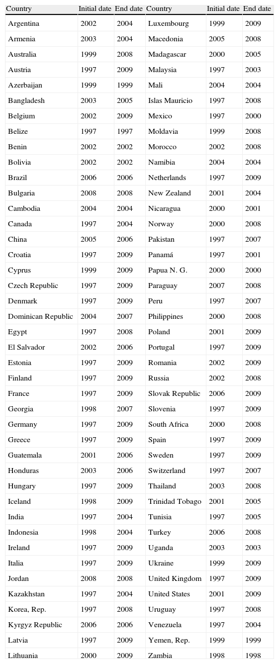
The final sample is described in Table 1, where we report the period for which the information from each country is available.
Sample composition.
| Country | Initial date | End date | Country | Initial date | End date |
| Argentina | 2002 | 2004 | Luxembourg | 1999 | 2009 |
| Armenia | 2003 | 2004 | Macedonia | 2005 | 2008 |
| Australia | 1999 | 2008 | Madagascar | 2000 | 2005 |
| Austria | 1997 | 2009 | Malaysia | 1997 | 2003 |
| Azerbaijan | 1999 | 1999 | Mali | 2004 | 2004 |
| Bangladesh | 2003 | 2005 | Islas Mauricio | 1997 | 2008 |
| Belgium | 2002 | 2009 | Mexico | 1997 | 2000 |
| Belize | 1997 | 1997 | Moldavia | 1999 | 2008 |
| Benin | 2002 | 2002 | Morocco | 2002 | 2008 |
| Bolivia | 2002 | 2002 | Namibia | 2004 | 2004 |
| Brazil | 2006 | 2006 | Netherlands | 1997 | 2009 |
| Bulgaria | 2008 | 2008 | New Zealand | 2001 | 2004 |
| Cambodia | 2004 | 2004 | Nicaragua | 2000 | 2001 |
| Canada | 1997 | 2004 | Norway | 2000 | 2008 |
| China | 2005 | 2006 | Pakistan | 1997 | 2007 |
| Croatia | 1997 | 2009 | Panamá | 1997 | 2001 |
| Cyprus | 1999 | 2009 | Papua N. G. | 2000 | 2000 |
| Czech Republic | 1997 | 2009 | Paraguay | 2007 | 2008 |
| Denmark | 1997 | 2009 | Peru | 1997 | 2007 |
| Dominican Republic | 2004 | 2007 | Philippines | 2000 | 2008 |
| Egypt | 1997 | 2008 | Poland | 2001 | 2009 |
| El Salvador | 2002 | 2006 | Portugal | 1997 | 2009 |
| Estonia | 1997 | 2009 | Romania | 2002 | 2009 |
| Finland | 1997 | 2009 | Russia | 2002 | 2008 |
| France | 1997 | 2009 | Slovak Republic | 2006 | 2009 |
| Georgia | 1998 | 2007 | Slovenia | 1997 | 2009 |
| Germany | 1997 | 2009 | South Africa | 2000 | 2008 |
| Greece | 1997 | 2009 | Spain | 1997 | 2009 |
| Guatemala | 2001 | 2006 | Sweden | 1997 | 2009 |
| Honduras | 2003 | 2006 | Switzerland | 1997 | 2007 |
| Hungary | 1997 | 2009 | Thailand | 2003 | 2008 |
| Iceland | 1998 | 2009 | Trinidad Tobago | 2001 | 2005 |
| India | 1997 | 2004 | Tunisia | 1997 | 2005 |
| Indonesia | 1998 | 2004 | Turkey | 2006 | 2008 |
| Ireland | 1997 | 2009 | Uganda | 2003 | 2003 |
| Italia | 1997 | 2009 | Ukraine | 1999 | 2009 |
| Jordan | 2008 | 2008 | United Kingdom | 1997 | 2009 |
| Kazakhstan | 1997 | 2004 | United States | 2001 | 2009 |
| Korea, Rep. | 1997 | 2008 | Uruguay | 1997 | 2008 |
| Kyrgyz Republic | 2006 | 2006 | Venezuela | 1997 | 2004 |
| Latvia | 1997 | 2009 | Yemen, Rep. | 1999 | 1999 |
| Lithuania | 2000 | 2009 | Zambia | 1998 | 1998 |
Regarding the variables, we have tried to be consistent with previous analogous research (Armstrong et al., 1998; Dreisbach, 2007; Manasse and Roubini, 2009; Yim and Mitchell, 2005). We have also taken into account the variables usually employed by the rating agencies Euromoney, Moody's, Standard and Poors and Fitch to assess the sovereign risk.
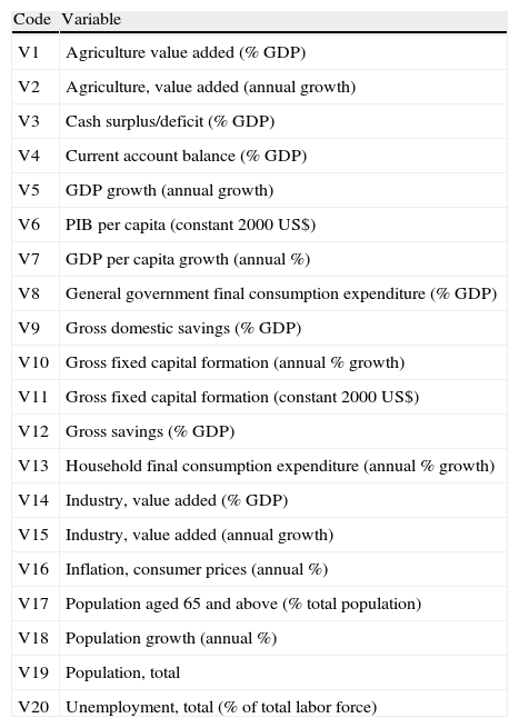
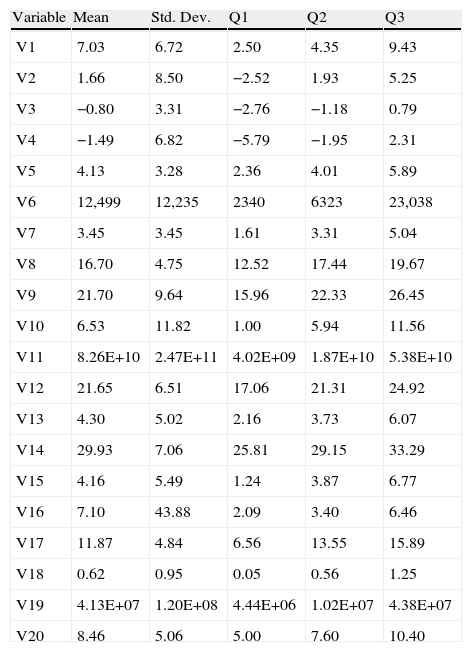
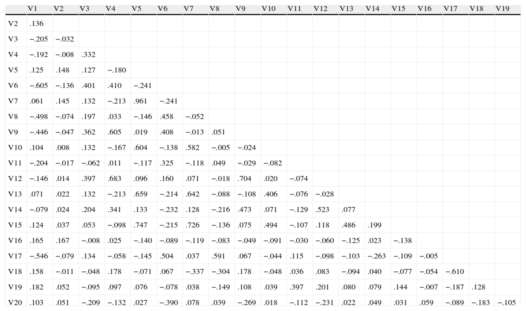
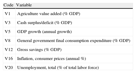
In Table 2 we present the list of our variables, in Table 3 we provide the definition of each variable and in Table 4 we show a descriptive analysis. Based on the correlation matrix reported in Table 5, we have selected the variables with the lowest correlation coefficient among them in order to keep the sample as big as possible.4 The list of the chosen variables is reported in Table 6.
List of variables.
| Code | Variable |
| V1 | Agriculture value added (% GDP) |
| V2 | Agriculture, value added (annual growth) |
| V3 | Cash surplus/deficit (% GDP) |
| V4 | Current account balance (% GDP) |
| V5 | GDP growth (annual growth) |
| V6 | PIB per capita (constant 2000 US$) |
| V7 | GDP per capita growth (annual %) |
| V8 | General government final consumption expenditure (% GDP) |
| V9 | Gross domestic savings (% GDP) |
| V10 | Gross fixed capital formation (annual % growth) |
| V11 | Gross fixed capital formation (constant 2000 US$) |
| V12 | Gross savings (% GDP) |
| V13 | Household final consumption expenditure (annual % growth) |
| V14 | Industry, value added (% GDP) |
| V15 | Industry, value added (annual growth) |
| V16 | Inflation, consumer prices (annual %) |
| V17 | Population aged 65 and above (% total population) |
| V18 | Population growth (annual %) |
| V19 | Population, total |
| V20 | Unemployment, total (% of total labor force) |
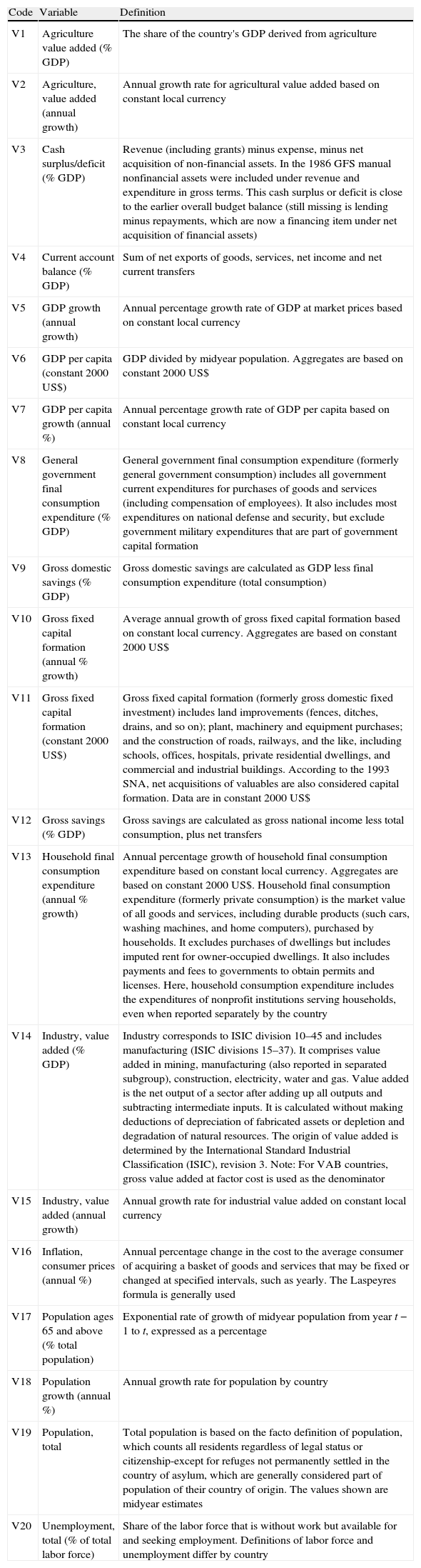
Definition of variables.
| Code | Variable | Definition |
| V1 | Agriculture value added (% GDP) | The share of the country's GDP derived from agriculture |
| V2 | Agriculture, value added (annual growth) | Annual growth rate for agricultural value added based on constant local currency |
| V3 | Cash surplus/deficit (% GDP) | Revenue (including grants) minus expense, minus net acquisition of non-financial assets. In the 1986 GFS manual nonfinancial assets were included under revenue and expenditure in gross terms. This cash surplus or deficit is close to the earlier overall budget balance (still missing is lending minus repayments, which are now a financing item under net acquisition of financial assets) |
| V4 | Current account balance (% GDP) | Sum of net exports of goods, services, net income and net current transfers |
| V5 | GDP growth (annual growth) | Annual percentage growth rate of GDP at market prices based on constant local currency |
| V6 | GDP per capita (constant 2000 US$) | GDP divided by midyear population. Aggregates are based on constant 2000 US$ |
| V7 | GDP per capita growth (annual %) | Annual percentage growth rate of GDP per capita based on constant local currency |
| V8 | General government final consumption expenditure (% GDP) | General government final consumption expenditure (formerly general government consumption) includes all government current expenditures for purchases of goods and services (including compensation of employees). It also includes most expenditures on national defense and security, but exclude government military expenditures that are part of government capital formation |
| V9 | Gross domestic savings (% GDP) | Gross domestic savings are calculated as GDP less final consumption expenditure (total consumption) |
| V10 | Gross fixed capital formation (annual % growth) | Average annual growth of gross fixed capital formation based on constant local currency. Aggregates are based on constant 2000 US$ |
| V11 | Gross fixed capital formation (constant 2000 US$) | Gross fixed capital formation (formerly gross domestic fixed investment) includes land improvements (fences, ditches, drains, and so on); plant, machinery and equipment purchases; and the construction of roads, railways, and the like, including schools, offices, hospitals, private residential dwellings, and commercial and industrial buildings. According to the 1993 SNA, net acquisitions of valuables are also considered capital formation. Data are in constant 2000 US$ |
| V12 | Gross savings (% GDP) | Gross savings are calculated as gross national income less total consumption, plus net transfers |
| V13 | Household final consumption expenditure (annual % growth) | Annual percentage growth of household final consumption expenditure based on constant local currency. Aggregates are based on constant 2000 US$. Household final consumption expenditure (formerly private consumption) is the market value of all goods and services, including durable products (such cars, washing machines, and home computers), purchased by households. It excludes purchases of dwellings but includes imputed rent for owner-occupied dwellings. It also includes payments and fees to governments to obtain permits and licenses. Here, household consumption expenditure includes the expenditures of nonprofit institutions serving households, even when reported separately by the country |
| V14 | Industry, value added (% GDP) | Industry corresponds to ISIC division 10–45 and includes manufacturing (ISIC divisions 15–37). It comprises value added in mining, manufacturing (also reported in separated subgroup), construction, electricity, water and gas. Value added is the net output of a sector after adding up all outputs and subtracting intermediate inputs. It is calculated without making deductions of depreciation of fabricated assets or depletion and degradation of natural resources. The origin of value added is determined by the International Standard Industrial Classification (ISIC), revision 3. Note: For VAB countries, gross value added at factor cost is used as the denominator |
| V15 | Industry, value added (annual growth) | Annual growth rate for industrial value added on constant local currency |
| V16 | Inflation, consumer prices (annual %) | Annual percentage change in the cost to the average consumer of acquiring a basket of goods and services that may be fixed or changed at specified intervals, such as yearly. The Laspeyres formula is generally used |
| V17 | Population ages 65 and above (% total population) | Exponential rate of growth of midyear population from year t−1 to t, expressed as a percentage |
| V18 | Population growth (annual %) | Annual growth rate for population by country |
| V19 | Population, total | Total population is based on the facto definition of population, which counts all residents regardless of legal status or citizenship-except for refuges not permanently settled in the country of asylum, which are generally considered part of population of their country of origin. The values shown are midyear estimates |
| V20 | Unemployment, total (% of total labor force) | Share of the labor force that is without work but available for and seeking employment. Definitions of labor force and unemployment differ by country |
Descriptive analysis.
| Variable | Mean | Std. Dev. | Q1 | Q2 | Q3 |
| V1 | 7.03 | 6.72 | 2.50 | 4.35 | 9.43 |
| V2 | 1.66 | 8.50 | −2.52 | 1.93 | 5.25 |
| V3 | −0.80 | 3.31 | −2.76 | −1.18 | 0.79 |
| V4 | −1.49 | 6.82 | −5.79 | −1.95 | 2.31 |
| V5 | 4.13 | 3.28 | 2.36 | 4.01 | 5.89 |
| V6 | 12,499 | 12,235 | 2340 | 6323 | 23,038 |
| V7 | 3.45 | 3.45 | 1.61 | 3.31 | 5.04 |
| V8 | 16.70 | 4.75 | 12.52 | 17.44 | 19.67 |
| V9 | 21.70 | 9.64 | 15.96 | 22.33 | 26.45 |
| V10 | 6.53 | 11.82 | 1.00 | 5.94 | 11.56 |
| V11 | 8.26E+10 | 2.47E+11 | 4.02E+09 | 1.87E+10 | 5.38E+10 |
| V12 | 21.65 | 6.51 | 17.06 | 21.31 | 24.92 |
| V13 | 4.30 | 5.02 | 2.16 | 3.73 | 6.07 |
| V14 | 29.93 | 7.06 | 25.81 | 29.15 | 33.29 |
| V15 | 4.16 | 5.49 | 1.24 | 3.87 | 6.77 |
| V16 | 7.10 | 43.88 | 2.09 | 3.40 | 6.46 |
| V17 | 11.87 | 4.84 | 6.56 | 13.55 | 15.89 |
| V18 | 0.62 | 0.95 | 0.05 | 0.56 | 1.25 |
| V19 | 4.13E+07 | 1.20E+08 | 4.44E+06 | 1.02E+07 | 4.38E+07 |
| V20 | 8.46 | 5.06 | 5.00 | 7.60 | 10.40 |
Correlation matrix.
| V1 | V2 | V3 | V4 | V5 | V6 | V7 | V8 | V9 | V10 | V11 | V12 | V13 | V14 | V15 | V16 | V17 | V18 | V19 | |
| V2 | .136 | ||||||||||||||||||
| V3 | −.205 | −.032 | |||||||||||||||||
| V4 | −.192 | −.008 | .332 | ||||||||||||||||
| V5 | .125 | .148 | .127 | −.180 | |||||||||||||||
| V6 | −.605 | −.136 | .401 | .410 | −.241 | ||||||||||||||
| V7 | .061 | .145 | .132 | −.213 | .961 | −.241 | |||||||||||||
| V8 | −.498 | −.074 | .197 | .033 | −.146 | .458 | −.052 | ||||||||||||
| V9 | −.446 | −.047 | .362 | .605 | .019 | .408 | −.013 | .051 | |||||||||||
| V10 | .104 | .008 | .132 | −.167 | .604 | −.138 | .582 | −.005 | −.024 | ||||||||||
| V11 | −.204 | −.017 | −.062 | .011 | −.117 | .325 | −.118 | .049 | −.029 | −.082 | |||||||||
| V12 | −.146 | .014 | .397 | .683 | .096 | .160 | .071 | −.018 | .704 | .020 | −.074 | ||||||||
| V13 | .071 | .022 | .132 | −.213 | .659 | −.214 | .642 | −.088 | −.108 | .406 | −.076 | −.028 | |||||||
| V14 | −.079 | .024 | .204 | .341 | .133 | −.232 | .128 | −.216 | .473 | .071 | −.129 | .523 | .077 | ||||||
| V15 | .124 | .037 | .053 | −.098 | .747 | −.215 | .726 | −.136 | .075 | .494 | −.107 | .118 | .486 | .199 | |||||
| V16 | .165 | .167 | −.008 | .025 | −.140 | −.089 | −.119 | −.083 | −.049 | −.091 | −.030 | −.060 | −.125 | .023 | −.138 | ||||
| V17 | −.546 | −.079 | .134 | −.058 | −.145 | .504 | .037 | .591 | .067 | −.044 | .115 | −.098 | −.103 | −.263 | −.109 | −.005 | |||
| V18 | .158 | −.011 | −.048 | .178 | −.071 | .067 | −.337 | −.304 | .178 | −.048 | .036 | .083 | −.094 | .040 | −.077 | −.054 | −.610 | ||
| V19 | .182 | .052 | −.095 | .097 | .076 | −.078 | .038 | −.149 | .108 | .039 | .397 | .201 | .080 | .079 | .144 | −.007 | −.187 | .128 | |
| V20 | .103 | .051 | −.209 | −.132 | .027 | −.390 | .078 | .039 | −.269 | .018 | −.112 | −.231 | .022 | .049 | .031 | .059 | −.089 | −.183 | −.105 |
Final selected variables.
| Code | Variable |
| V1 | Agriculture value added (% GDP) |
| V3 | Cash surplus/deficit (% GDP) |
| V5 | GDP growth (annual growth) |
| V8 | General government final consumption expenditure (% GDP) |
| V12 | Gross savings (% GDP) |
| V16 | Inflation, consumer prices (annual %) |
| V20 | Unemployment, total (% of total labor force) |
To soften the information, to get a more continuous distribution and to moderate the effect of outliers, we make a logistic transformation5 of the data (Pyle, 1999). This transformation scales all possible values between 0 and 1. The transformation is more-or-less linear in the middle range (around mean value), and has a smooth nonlinearity at both ends which ensures that all values are within the range. Then we process the information from 1997 to 2008 (our training sample) with the Matlab Som Toolbox tool. The first layer of the model has 588 input patterns (all countries in the sample) and the output layer is a bidimensional map of 12×10. The size of the map follows the recommendations of Kohonen (1993) and Kaski and Kohonen (1994). Thus, the number of connections or weights is 840 (7 variables multiplied by the size of the map) (Table 7).
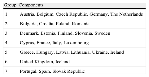
Classification of countries.
| Group | Components |
| 1 | Austria, Belgium, Czech Republic, Germany, The Netherlands |
| 2 | Bulgaria, Croatia, Poland, Romania |
| 3 | Denmark, Estonia, Finland, Slovenia, Sweden |
| 4 | Cyprus, France, Italy, Luxembourg |
| 5 | Greece, Hungary, Latvia, Lithuania, Ukraine, Ireland |
| 6 | United Kingdom, Iceland |
| 7 | Portugal, Spain, Slovak Republic |
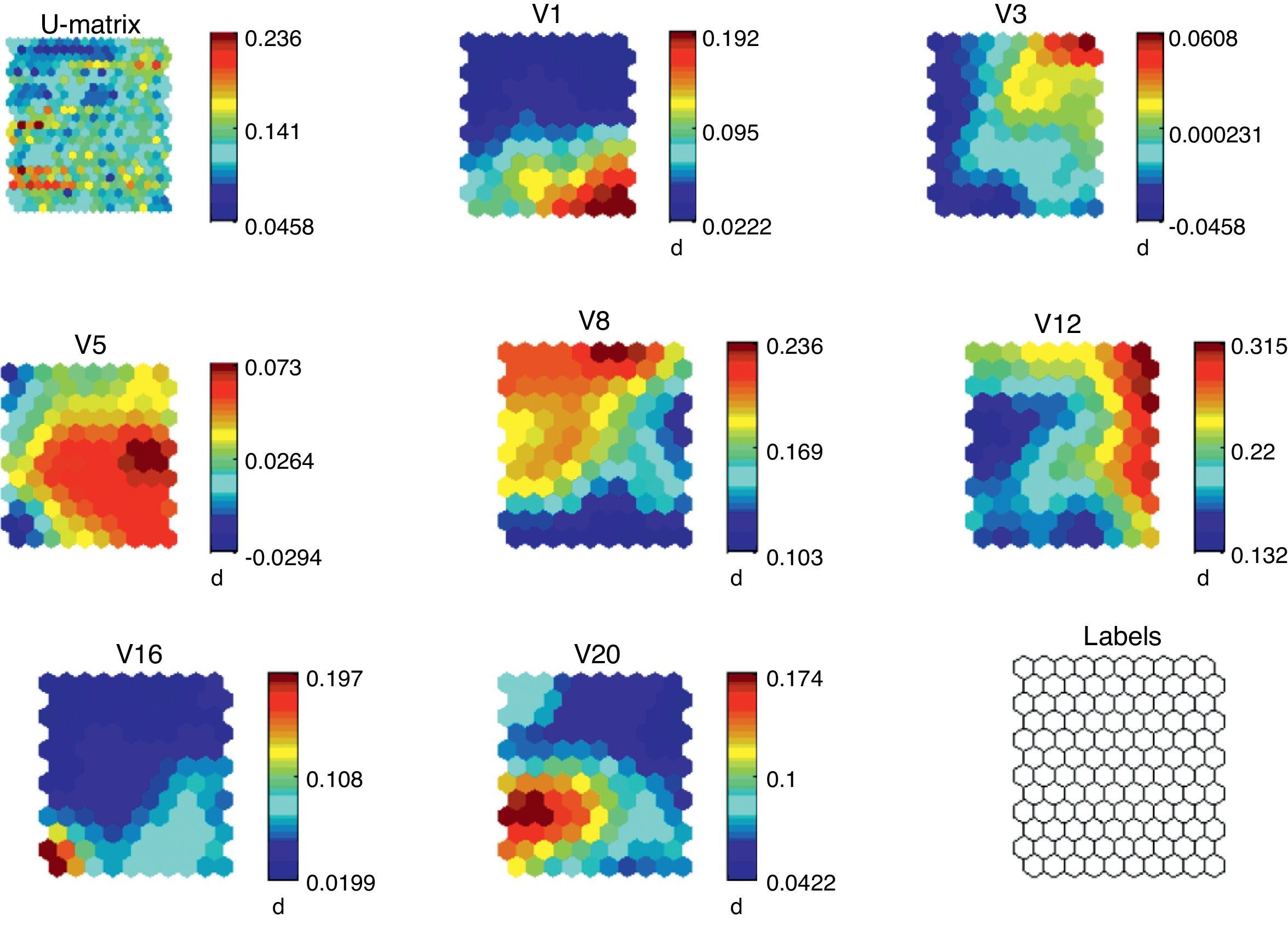
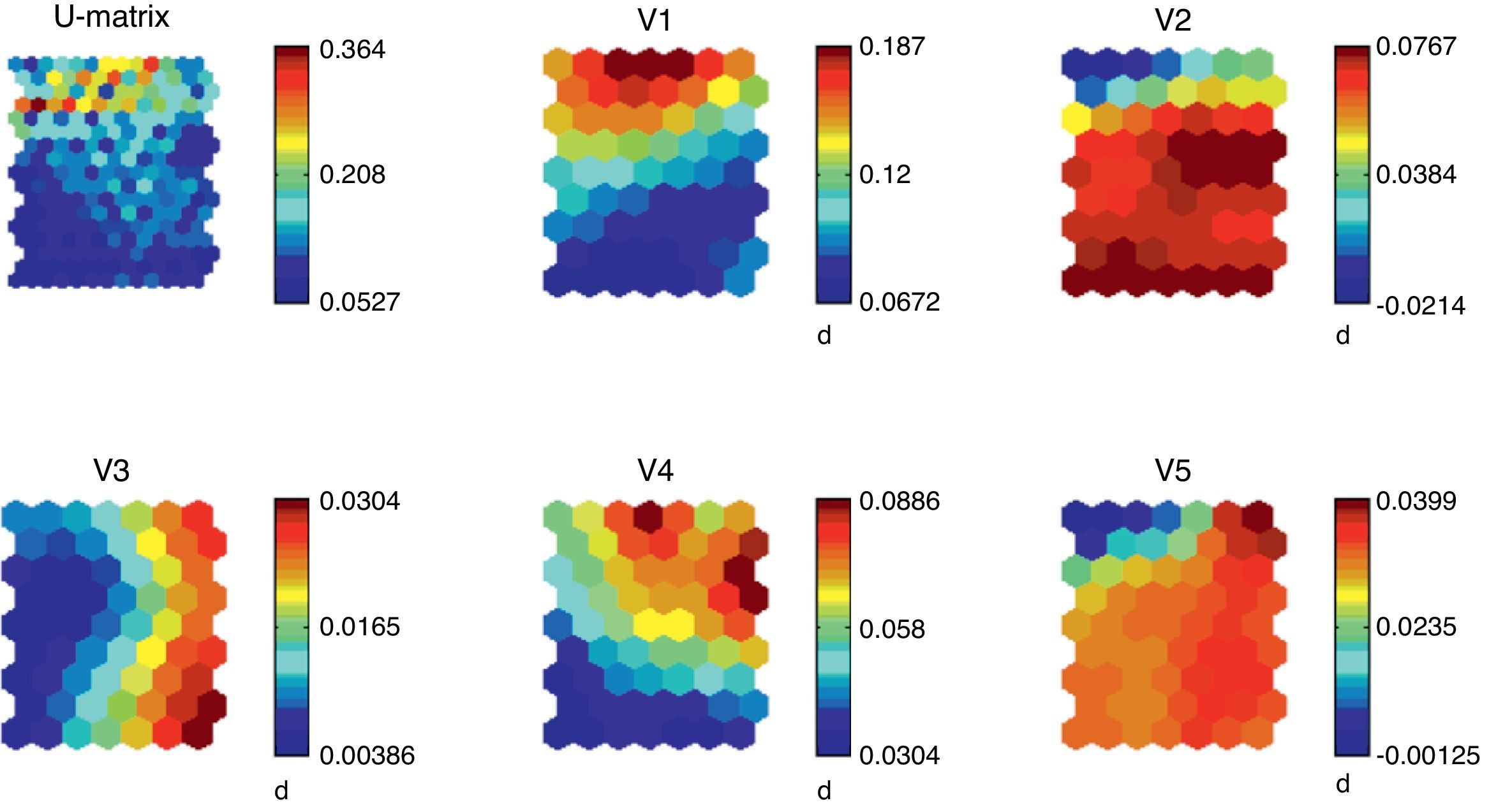
The results of the training of the model are shown in Fig. 2. We can note the so-called U-Matrix, with which we determine the different distances among the neurons through the training of the model. In the U-Matrix, the distance is reported by colors: light colors for short distances and dark colors for long distances. The other figures show the density function of the variables. For each variable we show the whole map of neurons and the value distribution in the map.
.")
If we analyze the overlapping and compare the different figures we can see the logic of the model from a mathematical point of view. For instance, high values of public deficit are linked to low values of the saving rate related to the GDP, high unemployment rates and low inflation rate. According to Fig. 2, all the variables are significant, which corroborates the selection of variables.
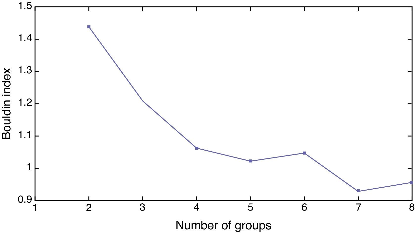
After training the model, we have to introduce and process the information from 2009 in order to sort the countries out (Khashman, 2010). A key decision is the one concerning the number of groups given that a too low number of groups would lead to internally too heterogeneous groups whereas a too high number of groups could result in the insufficient identification of common characteristics to several countries. The ideal number of groups is the one that maximizes intra-groups homogeneity whereas maximizes inter-groups heterogeneity. The K-means non-hierarchical clustering function is used to find an initial partitioning. K-Means is the least sensitive to outliers (Hair et al., 1999) and has been also used in other works like Moreno et al. (2006) to classify the Spanish mutual funds with SOM. There are some methods to determine the optimal number of groups (Fraley and Raftery, 1998), although in SOM one of the most widely used algorithms is the Davies–Bouldin index (Davies and Bouldin, 1979). This index is a function of the ratio within cluster variation to between cluster variations (Ingaramo et al., 2005). The smaller the index, the better the partition is. According to this index, the optimal number of groups of countries is seven as shown in Fig. 3.

We focus on the situation of the Euro-27 countries and, thus, in figure we report the results for these countries.6 We include Iceland because it was the first country deeply affected by the financial crisis in Europe and formally applied for EU membership in 2009. We also include Croatia because it will join the EU in July 2013 and Ukraine because of the strategic ties and the agreement signed with the EU to create a free trade area in 2013. Results are shown in Tables 8–10.
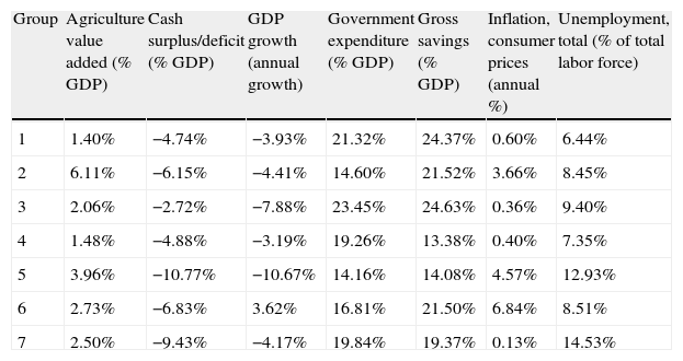
Mean values for each group of countries.
| Group | Agriculture value added (% GDP) | Cash surplus/deficit (% GDP) | GDP growth (annual growth) | Government expenditure (% GDP) | Gross savings (% GDP) | Inflation, consumer prices (annual %) | Unemployment, total (% of total labor force) |
| 1 | 1.40% | −4.74% | −3.93% | 21.32% | 24.37% | 0.60% | 6.44% |
| 2 | 6.11% | −6.15% | −4.41% | 14.60% | 21.52% | 3.66% | 8.45% |
| 3 | 2.06% | −2.72% | −7.88% | 23.45% | 24.63% | 0.36% | 9.40% |
| 4 | 1.48% | −4.88% | −3.19% | 19.26% | 13.38% | 0.40% | 7.35% |
| 5 | 3.96% | −10.77% | −10.67% | 14.16% | 14.08% | 4.57% | 12.93% |
| 6 | 2.73% | −6.83% | 3.62% | 16.81% | 21.50% | 6.84% | 8.51% |
| 7 | 2.50% | −9.43% | −4.17% | 19.84% | 19.37% | 0.13% | 14.53% |
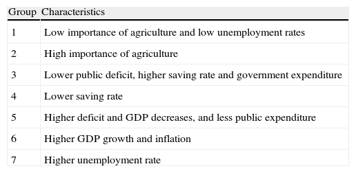
Main characteristics of each group of countries.
| Group | Characteristics |
| 1 | Low importance of agriculture and low unemployment rates |
| 2 | High importance of agriculture |
| 3 | Lower public deficit, higher saving rate and government expenditure |
| 4 | Lower saving rate |
| 5 | Higher deficit and GDP decreases, and less public expenditure |
| 6 | Higher GDP growth and inflation |
| 7 | Higher unemployment rate |
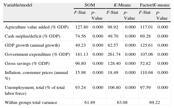
Comparison of the classification models. This table provides the F-statistics and the p-value of the most important variables. We also report the within groups variance of the three classification models.
| Variable/model | SOM | K-Means | Factor/K-means | |||
| F-Stat | p-Value | F-Stat | p-Value | F-Stat | p-Value | |
| Agriculture value added (% GDP) | 127.80 | 0.000 | 98.92 | 0.000 | 117.01 | 0.000 |
| Cash surplus/deficit (% GDP) | 74.56 | 0.000 | 49.70 | 0.000 | 69.28 | 0.000 |
| GDP growth (annual growth) | 49.23 | 0.000 | 82.57 | 0.000 | 125.61 | 0.000 |
| Government expenditure (% GDP) | 181.13 | 0.000 | 261.74 | 0.000 | 107.06 | 0.000 |
| Gross savings (% GDP) | 96.80 | 0.000 | 128.40 | 0.000 | 52.82 | 0.000 |
| Inflation, consumer prices (annual %) | 15.98 | 0.000 | 18.49 | 0.000 | 110.68 | 0.000 |
| Unemployment, total (% of total labor force) | 93.24 | 0.000 | 106.80 | 0.000 | 97.59 | 0.000 |
| Within groups total variance | 61.89 | 63.08 | 69.22 | |||
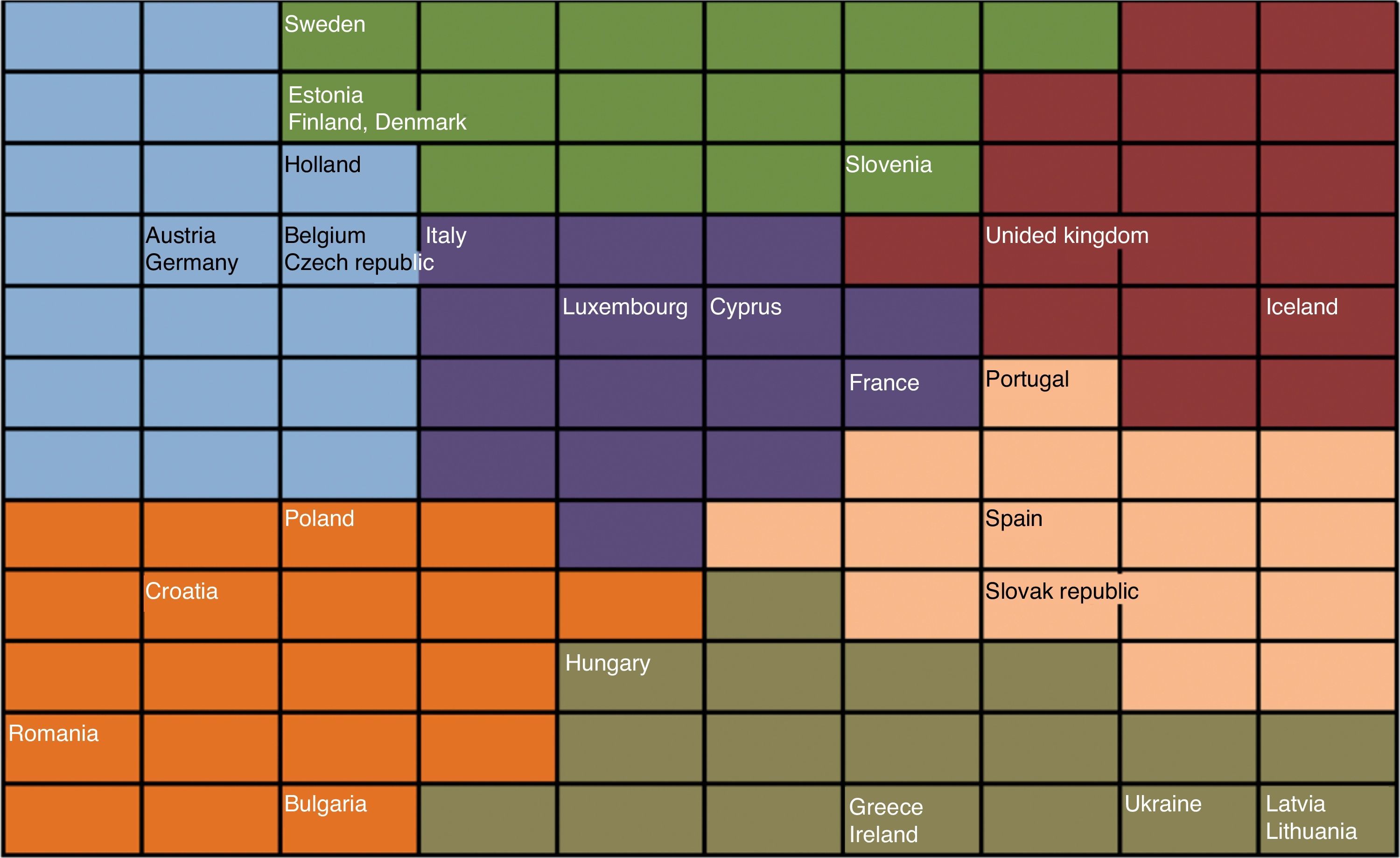
The main indicators of each country are reported in Table 8 and Fig. 4. In order to summarize the information of this table, in Table 9 we present the main characteristics of each group.

As shown in Fig. 4, the first group is made up by Holland, the Czech Republic, Belgium, Austria and Germany. Broadly speaking, this group of countries is Central-Europe nations. The second group includes the Western Europe countries recently joining or waiting for the EU membership. The third group is also quite geographical since it is made up by the Nordic countries and some other close countries such as Estonia or Slovenia (although Slovenia is also near to other groups, which is consistent with the geographical distance from the Nordic countries). Group 4 includes Luxembourg and a number of Mediterranean countries such as Italy, Cyprus and France. It is a relatively heterogeneous group since whereas Italy is close to the first group, France and Cyprus are near to countries such as Spain and Portugal.
The fifth group includes the countries in the most difficult situation: Greece, Hungary, Ireland, Ukraine, Latvia and Lithuania. Ireland was intervened by the EU in 2010 and the very adverse Greek situation is widely known. Ukraine, Latvia and Lithuania are in recession, and Hungary has suffered from severe problems on the public account that led the IMF to investigate a possible intentional manipulation and that resulted in a restatement of the public deficit from 4.5% to 7.5%. In the Group 6 we find the UK and Iceland. Although their unemployment rate, economic growth and public deficit is close to Greece or Ireland, their economic and financial characteristics, the large size of UK, and their good perspectives, they are likely to push them out of the crisis sooner than other countries. Nevertheless, there are some troublesome issues such as the overleverage. The last group would include Spain, Portugal and Slovakia. These are countries in financial troubles as shown by the international intervention in Portugal. 2010 has been a key year to assess the evolution of these countries: Portugal has moved closer to Greece and Ireland, and Spain is under huge European pressure to give unequivocal signs of public expenditure cut-offs and to dissipate the financial uncertainty.
3.3Assessment of the modelTo assess the goodness of the model, we need further tests. We compare our output with two clustering techniques: K-means cluster and a two-step factor analysis/K-means procedure. These methods have been used before to compare some unsupervised networks (Kiang, 2001; Kiang et al., 2006; Mingoti and Lima, 2006). K-Means is one of the most best-known unsupervised algorithms since it is a robust and easy-to-implement method. The two-step factor analysis/K-means procedure consists of the application of the factor analysis to reduce the data dimensions before applying the K-means clustering method.
The optimal model is the one that maximizes intra-groups homogeneity and inter-groups heterogeneity. It can be assessed by comparing the within cluster total variance. For a given number of clusters, the smaller the within cluster variance, the more homogeneous the clusters. Given the sensitivity of the cluster analysis to initial seeds (Milligan and Cooper, 1980), in the K-means procedure we use the same inputs than the SOM. In the factor/cluster method, we use a factor analysis with varimax rotation. In a first step we obtain three factors, which are the inputs in a K-means procedure. Table 10 shows the within-groups variance of the three methods. As reported, the F-statistic and the p-value of the most important variables are highly consistent across all the methods. Interestingly, SOM outperforms the K-means and the factor/cluster procedures according to the within-cluster variance.
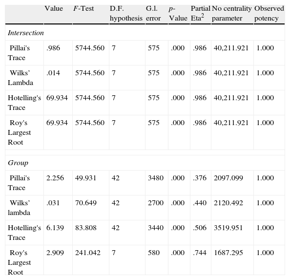
Finally, an interpretation about the weights of the network can be done with the so-called sensitivity analysis (Garson, 1991; Hunter et al., 2000; Rambhia et al., 1994; Zurada et al., 1994). Because of the complexity to determine the importance (or relation) of each input variable with the output of the model, the sensitivity analysis allows us to identify the most relevant variables. The ANOVA with the results of SOM model are reported in Table 11. We use four indicators to analyze the significance of the differences: Wilk's Lambda, Pillai's Trace, Hotelling's Trace and the Roy's Largest Root. All the indicators show that there are significant differences among the variables across the groups. High values of the first indicator or low values of the last three indicators point at differences among groups. As shown in Table 10, the mean of each group is significantly different.
Analysis of variance (ANOVA) of the country classification.
| Value | F-Test | D.F. hypothesis | G.l. error | p-Value | Partial Eta2 | No centrality parameter | Observed potency | |
| Intersection | ||||||||
| Pillai's Trace | .986 | 5744.560 | 7 | 575 | .000 | .986 | 40,211.921 | 1.000 |
| Wilks’ Lambda | .014 | 5744.560 | 7 | 575 | .000 | .986 | 40,211.921 | 1.000 |
| Hotelling's Trace | 69.934 | 5744.560 | 7 | 575 | .000 | .986 | 40,211.921 | 1.000 |
| Roy's Largest Root | 69.934 | 5744.560 | 7 | 575 | .000 | .986 | 40,211.921 | 1.000 |
| Group | ||||||||
| Pillai's Trace | 2.256 | 49.931 | 42 | 3480 | .000 | .376 | 2097.099 | 1.000 |
| Wilks’ lambda | .031 | 70.649 | 42 | 2700 | .000 | .440 | 2120.492 | 1.000 |
| Hotelling's Trace | 6.139 | 83.808 | 42 | 3440 | .000 | .506 | 3519.951 | 1.000 |
| Roy's Largest Root | 2.909 | 241.042 | 7 | 580 | .000 | .744 | 1687.295 | 1.000 |
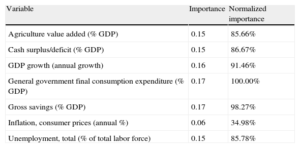
The sensitivity analysis is based on measuring the observed effect on an output Yj due to the change in an input Xi. The bigger the effect is, the more the sensitivity. Results reported in Table 12 show that the most influential variables are the public expenditure (as a proportion of GDP) and the saving rate (also as a proportion of GDP). The following variables in importance are the rate of GDP growth, the public deficit and the unemployment. On the contrary, the inflation rate and the importance of agriculture in GDP are the least significant variables.
Sensitivity analysis of the countries classification.
| Variable | Importance | Normalized importance |
| Agriculture value added (% GDP) | 0.15 | 85.66% |
| Cash surplus/deficit (% GDP) | 0.15 | 86.67% |
| GDP growth (annual growth) | 0.16 | 91.46% |
| General government final consumption expenditure (% GDP) | 0.17 | 100.00% |
| Gross savings (% GDP) | 0.17 | 98.27% |
| Inflation, consumer prices (annual %) | 0.06 | 34.98% |
| Unemployment, total (% of total labor force) | 0.15 | 85.78% |
The Spanish AA.CC. are regional entities with wide range of political and financial autonomy that show big differences in terms of financial balance. Although it has not been until recently that the macroeconomic unbalance of AA.CC. has drawn the attention of politicians and mass-media, academia had thoroughly studied their budgetary ability and their contribution to the whole national public expenditure (Martínez García and Colldeforns, 2003; Ríos et al., 2007; Sanz and Velázquez, 2001). The gap between the dramatic increments in the public expenditure of most of the AA.CC. and the objectives of Spain have forced the Spanish Government to pass a strict adjustment plan to cut-off the public deficit and to meet the European objectives.
In this Section we explore the financial differences across AA.CC. to identify the ones that should make the most effort to balance their public accounts and to assure their solvency. We aim to provide a tool to assess and to compare the financial situation of the AA.CC., in order to focus the effort on the most troublesome regions and to implement the necessary corrective policies.
As in the countries classification, the SOM method is a suitable way to identify the main similarities and differences across AA.CC. Peralta et al. (2000) and Alfaro Cortés et al. (2002) have utilized the SOM method for a socio-economic classification of the European regions, and Moreno and Olmeda (2007) and Jaráiz Cabanillas et al. (2012) do the same for the Valence region and for the central area of the Iberia Peninsula respectively. Our research goes a step forward not only in the variables we use but also in the objective since we do not intend a socio-economic classification but to identify the financial unbalances and the AA.CC. solvency threats. Thus, we focus on the economic variables to which the EU gives priority and we base in the conclusions, methods and recommendations of the above mentioned literature.
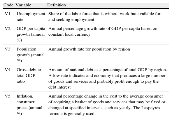
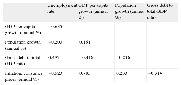
4.1Empirical design of the modelUnlike the national accounts of Section 3, macroeconomic information about Spanish AA.CC. is not so profuse. We have used the information available at the Spanish National Statistical Institute, the Statistical Institute of each AA.CC., Eurostat and the reports on the economic situation from the Saving Banks Foundation (FUNCAS) and the Bank of Spain. The variables have been selected consistently with previous research (Fernández Llera, 2006), with the rating agencies and with the EU recommendations (Table 13). In Table 14 we report the correlation matrix.
Variables considered in the Spanish regions classification.
| Code | Variable | Definition |
| V1 | Unemployment rate | Share of the labor force that is without work but available for and seeking employment |
| V2 | GDP per capita growth (annual %) | Annual percentage growth rate of GDP per capita based on constant local currency |
| V3 | Population growth (annual %) | Annual growth rate for population by region |
| V4 | Gross debt to total GDP ratio | Amount of national debt as a percentage of total GDP by region. A low rate indicates and economy that produces a large number of goods and services and probably profit enough to pay the debt interest |
| V5 | Inflation, consumer prices (annual %) | Annual percentage change in the cost to the average consumer of acquiring a basket of goods and services that may be fixed or changed at specified intervals, such as yearly. The Laspeyres formula is generally used |
Correlation matrix (Spanish classification).
| Unemployment rate | GDP per capita growth (annual %) | Population growth (annual %) | Gross debt to total GDP ratio | |
| GDP per capita growth (annual %) | −0.635 | |||
| Population growth (annual %) | −0.203 | 0.161 | ||
| Gross debt to total GDP ratio | 0.497 | −0.416 | −0.016 | |
| Inflation, consumer prices (annual %) | −0.523 | 0.783 | 0.233 | −0.314 |
The model has been developed with the Matlab Som Toolbox, based on the information on the AA.CC. from 2001 to 2009. Then, we test the model with the information for 2010. As previously, after loading all the variables in the model, we perform a logistic normalization to smooth the information and to increase the data continuity.
Since the model is a competitive network, it has only two layers: the input one and the output one. The input layer is made of 162 input patterns from the data of the 17 AA.CC. for nine years and nine more observations from Spain as a whole. The neurons of the input layer are connected through synaptic weights with all the neurons of the output layer. Thus, the information provided by each neuron from the input layer is sent to every neuron of the output layer. Likewise, each neuron of the output layer receives the same set of inputs from the input layer. The number of units of the output layer is a two-dimension map of 9×7; therefore, the number of connections or weight is 441.
The results of the model training are shown in Fig. 4. We present the U-Matrix that determines the distances among the neurons through training step, and the density functions of the six variables that we finally use. As in the country classification model, the colors of the U-Matrix represent the distance among the neurons, so that strong colors are representative of long distances and clear colors of lower distance among the neurons. For each variable Fig. 4 shows the whole map of neurons and their density functions. By overlapping and comparing the different figures we can note the logic of the model from an economic point of view. For example, high values of unemployment are matched with low or even negative variation of GDP, high debt levels and stagnation of the total population. All the variables considered are statistically significant.
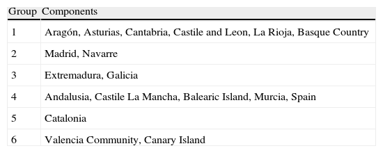
Concerning the ideal number of groups, we again use the Davies–Bouldin index. The optimal number of clusters that maximizes the within-groups homogeneity and the between-groups heterogeneity is six. In Tables 15–17 and in Figs. 5 and 6 we provide the results of the model for 2010.
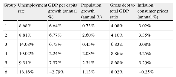
Mean values for each AA.CC.
| Group | Unemployment rate | GDP per capita growth (annual %) | Population growth (annual %) | Gross debt to total GDP ratio | Inflation, consumer prices (annual %) |
| 1 | 8.68% | 6.64% | 0.73% | 4.08% | 3.02% |
| 2 | 8.81% | 6.77% | 2.60% | 4.10% | 3.35% |
| 3 | 14.08% | 6.73% | 0.45% | 6.83% | 3.08% |
| 4 | 19.02% | 2.24% | 2.08% | 8.86% | 3.25% |
| 5 | 9.31% | 7.37% | 2.34% | 8.68% | 3.29% |
| 6 | 18.16% | −2.79% | 1.13% | 8.02% | −0.25% |
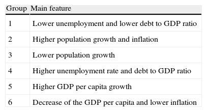
Main characteristics of each group of AA.CC.
| Group | Main feature |
| 1 | Lower unemployment and lower debt to GDP ratio |
| 2 | Higher population growth and inflation |
| 3 | Lower population growth |
| 4 | Higher unemployment rate and debt to GDP ratio |
| 5 | Higher GDP per capita growth |
| 6 | Decrease of the GDP per capita and lower inflation |
.")

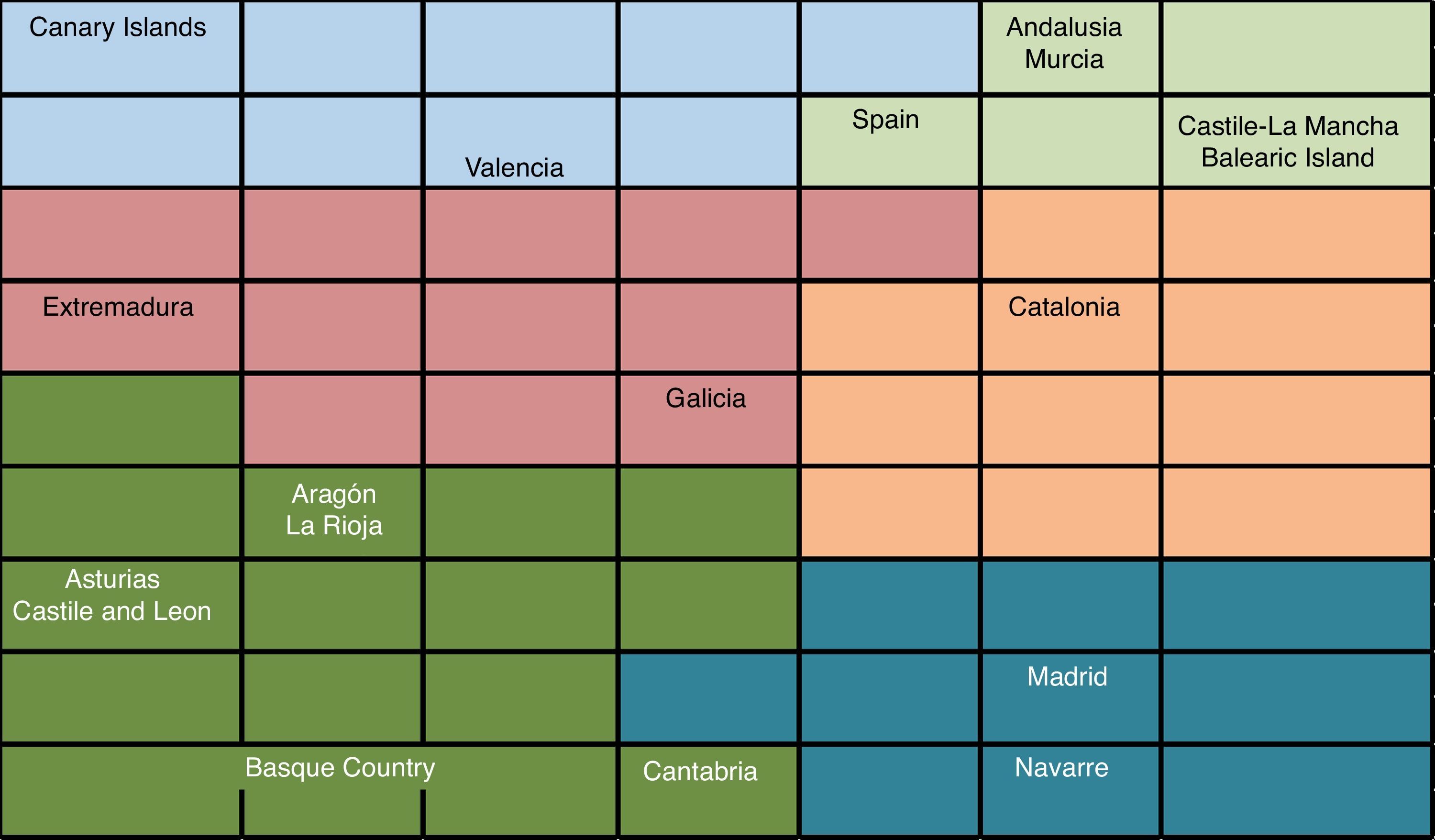
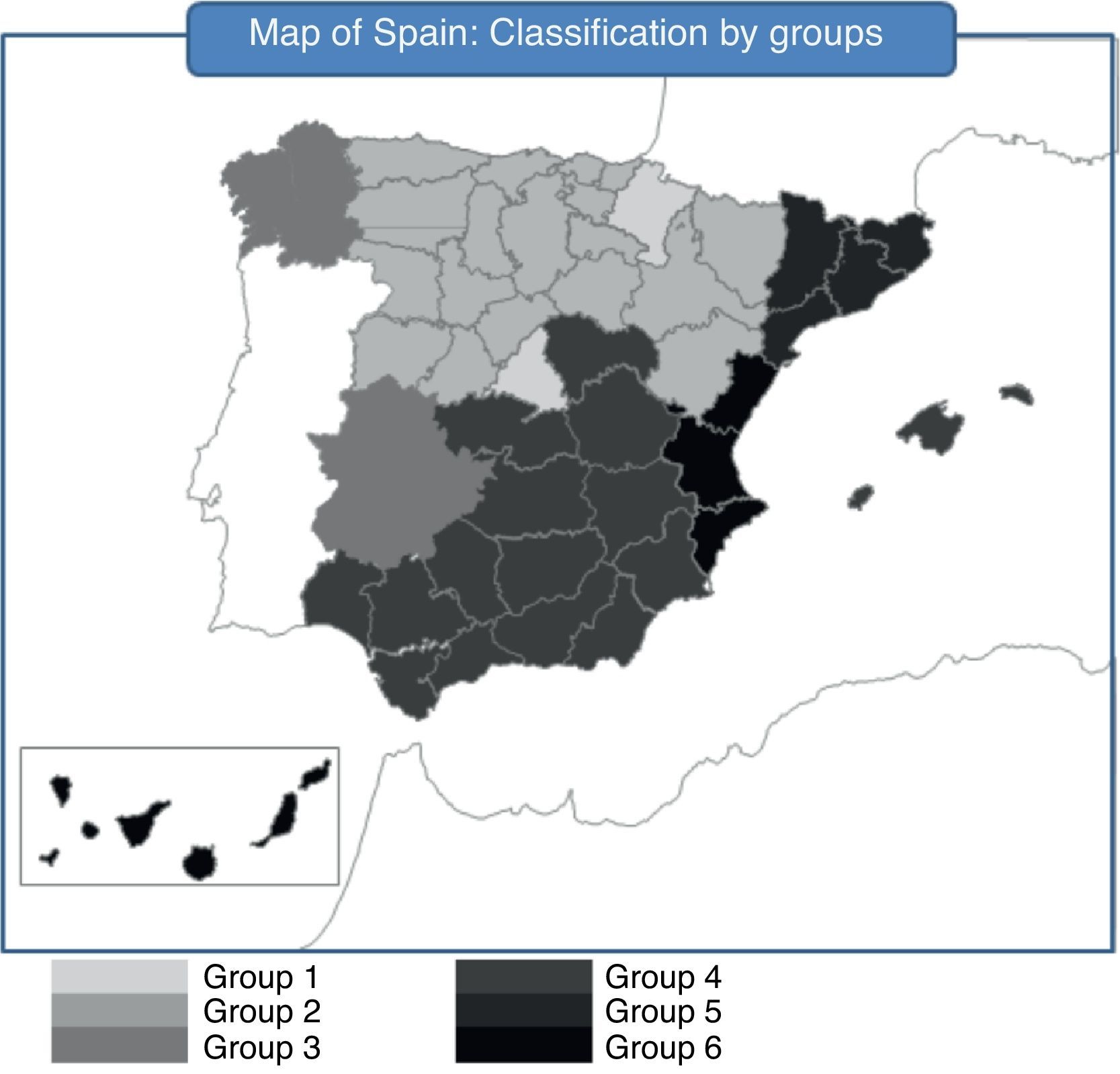
At the end of 2010, the AA.CC. with the best situation were Asturias, Aragón, Castile and Leon, La Rioja, the Basque Country and Cantabria. This group is characterized for an unemployment rate lower than the other groups, reduced debt level and a widespread increase of their GDP and inflation during 2010. Nevertheless, there are some differences inside the group. The Basque Country is the region with the best economic situation in Spain. Cantabria can also be considered in an economic recovery stage. Asturias and Castile and Leon are better placed than the national average but they show higher unemployment rates and less GDP growth. In spite of being included in this first group, Aragón and La Rioja have common characteristics with the Group 3. Group 2 is made of Madrid and Navarre. They show higher population growth in 2010.
Groups 3 and 4 are in an intermediate position. Inside the Group 3, Extremadura is close to the Group 1, being only different in terms of unemployment. Galicia is a rather peculiar case. It occupies a central position and relatively far from the other AA.CC., which means that it has some characteristics in common with several groups and it is not easy to include it into a specific group.
The next group by solvency and financial quality is the Group 5, formed only by Catalonia. This region is one of the most leveraged and during 2010 it issued a great amount of debt increasing the proportion of debt to GDP from 11.9% to 16.2%. Since the Catalonia GDP only increased in 1.16% in 2010, these data give a clear idea of its over-leverage. Nonetheless, the population of Catalonia grows yearly and the unemployment rate is under the Spanish average.
Groups 6 and 4 have in common a worrying feature since the unemployment rate is nearby 20%. The situation of Group 6 is even worse, with Valencia and the Canary Islands having worse growth in GDP, population and inflation than Andalusia, Castile-La Mancha, Balearic Island and Murcia.
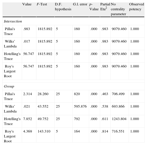
As in the countries analysis, we test the significance of the model through the ANOVA analysis and we analyze the importance of each variable through the sensitivity analysis. The ANOVA analysis reported in Table 18 corroborates the heterogeneity among groups and the homogeneity within groups.
Analysis of variance (ANOVA) of the Spanish AA.CC. classification.
| Value | F-Test | D.F. hypothesis | G.l. error | p-Value | Partial Eta2 | No centrality parameter | Observed potency | |
| Intersection | ||||||||
| Pillai's Trace | .983 | 1815.892 | 5 | 160 | .000 | .983 | 9079.460 | 1.000 |
| Wilks’ Lambda | .017 | 1815.892 | 5 | 160 | .000 | .983 | 9079.460 | 1.000 |
| Hotelling's Trace | 56.747 | 1815.892 | 5 | 160 | .000 | .983 | 9079.460 | 1.000 |
| Roy's Largest Root | 56.747 | 1815.892 | 5 | 160 | .000 | .983 | 9079.460 | 1.000 |
| Group | ||||||||
| Pillai's Trace | 2.314 | 28.260 | 25 | 820 | .000 | .463 | 706.499 | 1.000 |
| Wilks’ Lambda | .021 | 43.552 | 25 | 595.876 | .000 | .538 | 693.866 | 1.000 |
| Hotelling's Trace | 7.852 | 49.752 | 25 | 792 | .000 | .611 | 1243.804 | 1.000 |
| Roy's Largest Root | 4.369 | 143.310 | 5 | 164 | .000 | .814 | 716.551 | 1.000 |
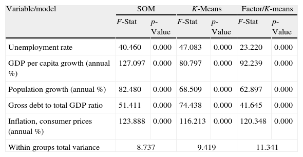
Table 19 reports the comparison among the SOM results and both the K-means and the factor/cluster procedures. Similar to the country classification model, the significance of the main variables is comparable and SOM provides the lowest variance among groups.
Comparison of the AA.CC. classification models.
| Variable/model | SOM | K-Means | Factor/K-means | |||
| F-Stat | p-Value | F-Stat | p-Value | F-Stat | p-Value | |
| Unemployment rate | 40.460 | 0.000 | 47.083 | 0.000 | 23.220 | 0.000 |
| GDP per capita growth (annual %) | 127.097 | 0.000 | 80.797 | 0.000 | 92.239 | 0.000 |
| Population growth (annual %) | 82.480 | 0.000 | 68.509 | 0.000 | 62.897 | 0.000 |
| Gross debt to total GDP ratio | 51.411 | 0.000 | 74.438 | 0.000 | 41.645 | 0.000 |
| Inflation, consumer prices (annual %) | 123.888 | 0.000 | 116.213 | 0.000 | 120.348 | 0.000 |
| Within groups total variance | 8.737 | 9.419 | 11.341 | |||
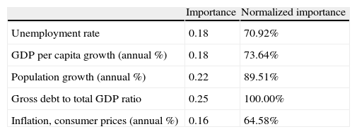
The sensitivity analysis reported in Table 20 shows that the debt-to-GDP ratio is the most significant variable. Our analysis shows the different situation of the macroeconomic situation of several Spanish AA.CC. It is not surprising that on September 2011 the Fitch rating agency downgraded the debt of Andalusia, Canary Island, Catalonia, Murcia and Valencia (the AA.CC. in the worst groups in our classification) and on October, 2011 Moody's downgraded the long-term debt rating of ten AA.CC., with a specially impact on Catalonia, Valencia and Castile-La Mancha. This generalized downgrading is likely to have affected the rating of the Spanish debt, which has been downgraded in 2011 and 2012.
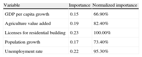
Sensitivity analysis of the AA.CC classification.
| Importance | Normalized importance | |
| Unemployment rate | 0.18 | 70.92% |
| GDP per capita growth (annual %) | 0.18 | 73.64% |
| Population growth (annual %) | 0.22 | 89.51% |
| Gross debt to total GDP ratio | 0.25 | 100.00% |
| Inflation, consumer prices (annual %) | 0.16 | 64.58% |
The classification of the Spanish AA.CC. and the study of their influence on the whole Spanish solvency can be complemented with an analogous analysis of other countries with a similar regional structure. Thus, we now present the results of our model for Germany and its 16 federal states or Bundesländer. With this analysis, we can test to which extent the situation of each regional entity impacts on the financial situation of the whole country. The choice of Germany has not been casual. Although German states have the consideration of NUT-1 and the AA.CC. have the consideration of NUT-2 according to the Nomenclature of the Territorial Units Statistics used by the EU, Spanish AA.CC. and German states play actually a comparable role. Likewise, the different economic situation of Germany in comparison with Spain allows testing the positive or negative effect for the whole country of the macroeconomic regional situation.
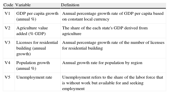
The variables we use are displayed in Table 21.7 The information sources are Eurostat, the OECD, and the Statistisches Bundesamt (German National Institute of Statistics). Although data sources are not exactly the same than the Spanish ones, we develop a model with a comparable explanatory capacity. We have information for all the 16 German states between 1996 and 2009. As previously, the model is built with information until 2008 (training sample) and we use the information from 2009 to perform the classification of the states (test sample).
Variables considered in the German states classification.
| Code | Variable | Definition |
| V1 | GDP per capita growth (annual %) | Annual percentage growth rate of GDP per capita based on constant local currency |
| V2 | Agriculture value added (% GDP) | The share of the each state's GDP derived from agriculture |
| V3 | Licenses for residential building (annual growth) | Annual percentage growth rate of the number of licenses for residential building |
| V4 | Population growth (annual %) | Annual growth rate for population by region |
| V5 | Unemployment rate | Unemployment refers to the share of the labor force that is without work but available for and seeking employment |
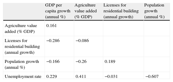
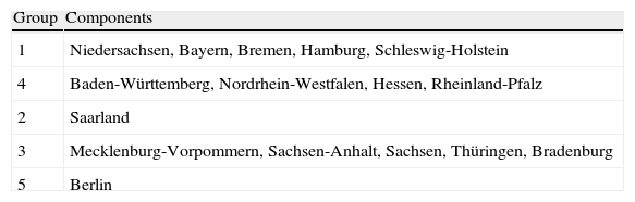
In Table 22 we provide the correlation matrix among the five variables we use. One can note the low correlation among them, so that multicolinearity is not a relevant concern in our analysis. The resulting German map is reported in Figs. 7 and 8, with an ideal number of five groups. In Table 23 we detail the composition of every group of states.
Correlations matrix (Germany classification).
| GDP per capita growth (annual %) | Agriculture value added (% GDP) | Licenses for residential building (annual growth) | Population growth (annual %) | |
| Agriculture value added (% GDP) | 0.161 | |||
| Licenses for residential building (annual growth) | −0.286 | −0.086 | ||
| Population growth (annual %) | −0.166 | −0.26 | 0.189 | |
| Unemployment rate | 0.229 | 0.411 | −0.031 | −0.607 |


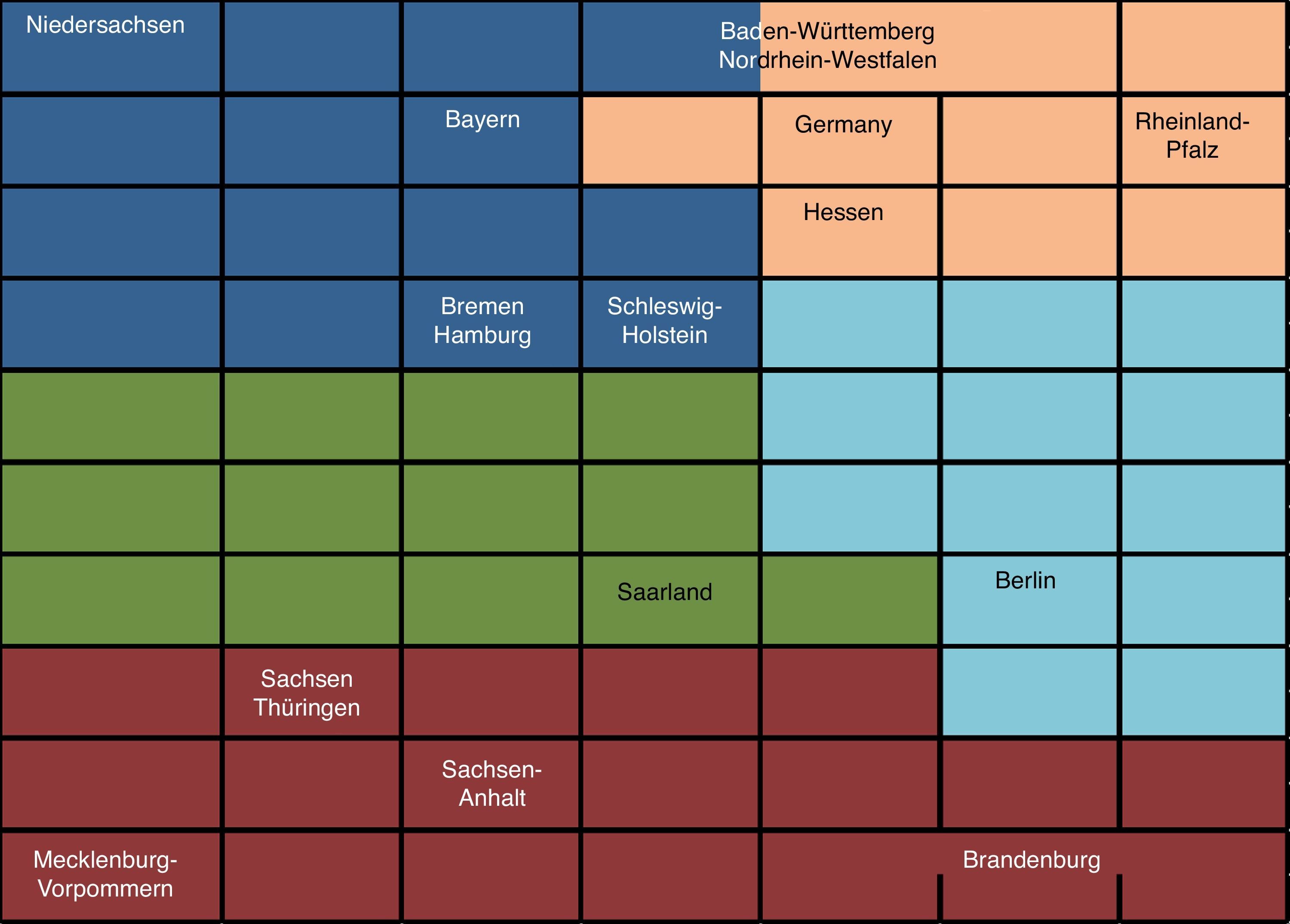
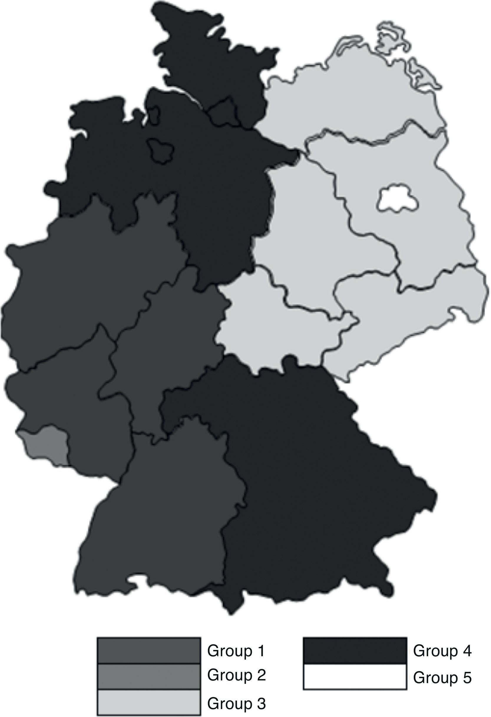
Our results show that nine States included in Groups 1 and 2 – the most solvent ones – come from the former Federal Republic of Germany (Tables 23–25 and Fig. 8). On the contrary, the six states included in the Groups 4 and 5 – the ones with the lowest solvency – are located in the Eastern side of the country. This shows that, after the process of reunification of the country in the 1990s, the efforts of the EU and of the German Government have not managed still to bridge the gap of development across the states. This result is coherent with Kronthaler (2003), who show the persistence of differences between both zones of Germany in terms of GDP growth and unemployment rate (Fig. 9).
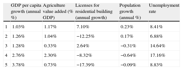
Mean values for each group (German states).
| GDP per capita growth (annual %) | Agriculture value added (% GDP) | Licenses for residential building (annual growth) | Population growth (annual %) | Unemployment rate | |
| 1 | 1.03% | 1.17% | 7.10% | 0.23% | 8.41% |
| 2 | 1.26% | 1.04% | −12.25% | 0.17% | 6.88% |
| 3 | 1.28% | 0.33% | 2.64% | −0.31% | 14.64% |
| 4 | 2.76% | 2.30% | −8.32% | −0.64% | 17.16% |
| 5 | 3.78% | 0.73% | −17.39% | −0.09% | 8.83% |
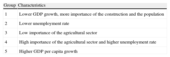
Main characteristics of each group (German states).
| Group | Characteristics |
| 1 | Lower GDP growth, more importance of the construction and the population |
| 2 | Lower unemployment rate |
| 3 | Low importance of the agricultural sector |
| 4 | High importance of the agricultural sector and higher unemployment rate |
| 5 | Higher GDP per capita growth |

The Saarland state is in an intermediate position. This small state, located between the French Lorraine and Luxembourg, suffers from 2008 in after from a substantial increase of unemployment, partially due to the fall of public and residential construction. It has been the German state with the highest GDP decrease in 2009.
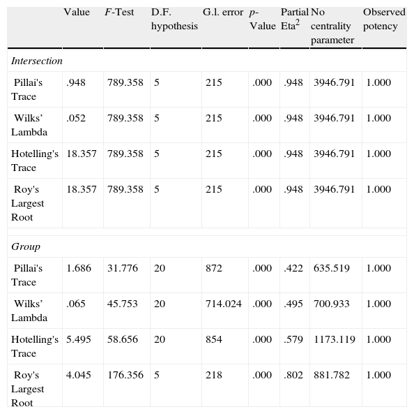
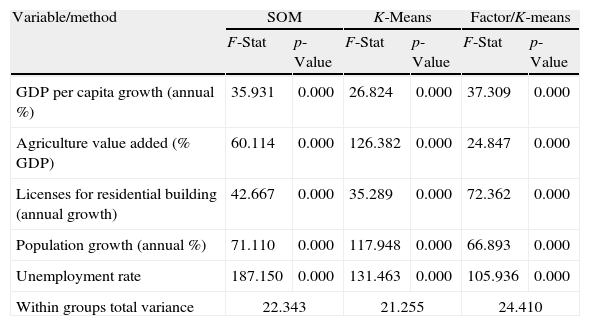
The sensitivity analysis (Table 26) shows that the most relevant variable is the licenses for residential buildings, followed by the unemployment rate, the value added by the agriculture to the GDP, the population growth and, finally, the GDP annual growth. The results of the ANOVA analysis (Table 27) corroborate the discriminatory power of the model and show significant differences among the groups. Again, the comparison with some more traditional techniques such as cluster analysis or factor analysis (Table 28) shows that SOM provides consistent results.
Analysis of variance (ANOVA) of the classification of German states.
| Value | F-Test | D.F. hypothesis | G.l. error | p-Value | Partial Eta2 | No centrality parameter | Observed potency | |
| Intersection | ||||||||
| Pillai's Trace | .948 | 789.358 | 5 | 215 | .000 | .948 | 3946.791 | 1.000 |
| Wilks’ Lambda | .052 | 789.358 | 5 | 215 | .000 | .948 | 3946.791 | 1.000 |
| Hotelling's Trace | 18.357 | 789.358 | 5 | 215 | .000 | .948 | 3946.791 | 1.000 |
| Roy's Largest Root | 18.357 | 789.358 | 5 | 215 | .000 | .948 | 3946.791 | 1.000 |
| Group | ||||||||
| Pillai's Trace | 1.686 | 31.776 | 20 | 872 | .000 | .422 | 635.519 | 1.000 |
| Wilks’ Lambda | .065 | 45.753 | 20 | 714.024 | .000 | .495 | 700.933 | 1.000 |
| Hotelling's Trace | 5.495 | 58.656 | 20 | 854 | .000 | .579 | 1173.119 | 1.000 |
| Roy's Largest Root | 4.045 | 176.356 | 5 | 218 | .000 | .802 | 881.782 | 1.000 |
Comparison of the German states classification models.
| Variable/method | SOM | K-Means | Factor/K-means | |||
| F-Stat | p-Value | F-Stat | p-Value | F-Stat | p-Value | |
| GDP per capita growth (annual %) | 35.931 | 0.000 | 26.824 | 0.000 | 37.309 | 0.000 |
| Agriculture value added (% GDP) | 60.114 | 0.000 | 126.382 | 0.000 | 24.847 | 0.000 |
| Licenses for residential building (annual growth) | 42.667 | 0.000 | 35.289 | 0.000 | 72.362 | 0.000 |
| Population growth (annual %) | 71.110 | 0.000 | 117.948 | 0.000 | 66.893 | 0.000 |
| Unemployment rate | 187.150 | 0.000 | 131.463 | 0.000 | 105.936 | 0.000 |
| Within groups total variance | 22.343 | 21.255 | 24.410 | |||
We could show the dynamic evolution of the groups of German states. Unlike Spain, Germany as a whole country would be included during 2009 in the group of states with the best financial situation. During that year the GDP per capita, the population, and the licenses for residential building have increased in Germany, and the unemployment rate has fallen.
Thus, in spite of the differences across the German states, our results show that the German regions are in a significantly better economic situation than their Spanish counterparts. Consequently, whereas the aggregation effect on the whole country is positive in Germany, the troublesome situation of Spain can be attributed, at least partially, to the financial weakness of its AA.CC.
6Concluding remarksSelf-organizing maps are a very useful tool for the classification of countries and regions based on their economic indicators. Using this method and a set of the usual macroeconomic variables, in this paper we analyze and compare the financial situation of the European countries in 2009 to obtain groups of countries conditional on their capacity to meet their financial commitments. Our results show the existence of several groups of countries, each one of them with specific characteristics. We also find that Government expenditure and the saving rate are the most influential variables on the macroeconomic financial imbalances.
We also study the influence of the macroeconomic situation of each Spanish AA.CC. and German states on the national situation. We find that the macroeconomic situation of the regional entities is a key determinant of the country financial (im)balance. Therefore, the identification of the regions that need the most demanding economic and social policies could alleviate the incidence of the current financial crisis.
Our research provides interesting insights for policymakers. The debate around the role played by the rating agencies in the financial crisis requires more and better methods of processing country-level information. From this perspective, our paper provides a complementary method to analyze the international macroeconomic financial situation. Yet, the identification of groups of similar countries can allow discovering possible channels of financial contagion and financial turbulences propagation across countries. Thus, our model could serve as an early warning system for some countries when the counterpart countries get into financial troubles.
In the same vein, the enlargement of the EU can be eased through diagnosing and forecasting the future financial situation of the candidate countries in order to avoid any destabilization effect. In addition, the identification of the regional disparities within European countries can lead to focus on the countries and regions in the most need of receiving European financial help.
From a microeconomic point of view, our research is also useful for banks and other institutional investors since the international risk map can be a relevant input to assess the risk exposure of each institution. This tool would be complementary to the stress tests and other analyses of sovereign risk carried out by national and international financial supervisors in recent months.
A more in detail presentation of the main yardsticks throughout the financial crisis can be found in the ECB website http://www.ecb.int/ecb/html/crisis.es.html.
The authors are grateful to Martí Sagarra, two anonymous referees, Francisco González (editor), the participants in the XX Finance Forum held in Oviedo, and the financial support provided by the Spanish Ministry of Science and Innovation (ECO2011-29144-C03-01). All the remaining errors are our only responsibility.
http://www.eba.europa.eu/EU-wide-stress-testing/2011/2011-EU-wide-stress-test-results.aspx.
http://ec.europa.eu/eurostat/ramon/nomenclatures/index.cfm?TargetUrl=LST_NOM_DTL&StrNom=NUTS_33&StrLanguageCode=EN∬PcKey=&StrLayoutCode=HIERARCHIC.
Although multicollinearity is not a big issue in SOM models, since not all the variables are available for all the countries throughout the analyzed period, by focusing on a selection of variables we manage to keep as many countries as possible.
The logistic transformation is also known as a softmax transformation.
Malta was excluded because the information was not available.
The variable “Licenses for construction of residential buildings” may seem weird but it is a variable with high historical importance in the German economy since the end of the World War II.

