


In this paper we study the equity premium predictability in eleven EuroZone countries. Besides some traditional predictive variables, we have also chosen two other that, to our knowledge, have never been previously used in the literature: the change in the OECD normalized composite leading indicator, and the change in the OECD business confidence indicator. The models based on the OECD variables outperform the historical average, in particular during the early stages of the recent financial crisis. We also show that the forecasts, based on these predictors, provide substantial utility gains for a mean-variance investor.
The theme of stock return predictability has been widely studied in the financial literature, but it remains highly controversial. Some authors argue that macroeconomic and financial variables can be used to forecast stock returns, while others assert that the evidence of predictability is illusory, because models are unstable and could not have been used by an investor to profitably time the market. This subject is relevant, not only to financial researchers, but also to asset managers and other investors that should take into account the potential existence of stock return predictability in their investment decisions.
In the United States, there are studies that report the presence of stock return predictability, based on a wide set of macroeconomic and financial variables, such as the dividend yield (Pettenuzzo and Timmermann, 2011; Neely et al., 2014; Lewellen, 2004), price dividend ratios (Bingsbergen and Koijen, 2010; Neely et al., 2014; Campbell and Yogo, 2006), valuation ratios (Lewellen, 2004; Campbell and Yogo, 2006), payout yields (Boudoukh et al., 2007), dividend growth ratios (Bingsbergen and Koijen, 2010), price earnings ratios (Rapach and Wohar, 2006), interest rates (Pettenuzzo and Timmermann, 2011; Ang and Bekaert, 2007; Campbell and Hamao, 1992), the term spread (Rapach and Wohar, 2006), the consumption-wealth ratio (Lettau and Ludvigson, 2001; Guo, 2002; Corte et al., 2010; Hahn and Lee, 2006), the output gap (Cooper and Priestley, 2009), the ratio of share prices to GDP (Rangvid, 2006), the stock variance (Guo, 2002) and expected business conditions (Campbell and Diebold, 2009). On the other hand, Goyal and Welch (2008) conducted a very comprehensive study of U.S. equity premium predictability, using a wide set of variables, and concluded that predictability was restricted to specific time periods, and that it disappeared in the most recent part of their sample.
Research on equity premium predictability outside the United States is more scarce and focuses mainly on developed countries. Papers that address this theme include, among others, Corte et al. (2010) (United States, United Kingdom, France and Japan), Harvey (1991) (16 OECD countries and Hong Kong), Cutler et al. (1991) (13 developed countries), Campbell and Hamao (1992) (United States and Japan), Ang and Bekaert (2007) (United States, United Kingdom, Germany and France), Kellard et al. (2010) (United States and United Kingdom), Paye and Timmermann (2006) (United States and United Kingdom), and Henkel et al. (2011) (G7 countries). Rapach et al. (2005) studied stock return predictability in twelve developed countries, using a wide set of variables, and concluded that interest rates are the most consistent predictors across all countries. Rapach et al. (2013) tested the lead-lag relationship between the U.S. and several developed stock markets, and found that the United States leads international stock markets. To our knowledge, the most comprehensive paper on international stock return predictability was conducted by Hjalmarsson (2010) who studied 24 developed and 16 developing countries. He concluded that short-term interest rates and term spreads are robust predictors of equity premia in developed countries, and that the dividend price ratios also show some predictive ability, for both emerging and developed countries.
In this paper, we study equity premia predictability in eleven EuroZone countries. The EuroZone is formed by a relatively homogeneous group of countries that share a common currency, and trade large volumes of goods and services. Furthermore, some of these countries were strongly affected by the recent financial crisis, and their GDP is still clearly below the pre-crisis level.
We have chosen, as forecasting variables, the dividend yield, the short-term interest rate, the long-term bond yield, the change in the OECD normalized composite leading indicator, and the change in the OECD business confidence indicator. Our choice was motivated by the fact that the dividend yield and the interest rates were widely used in previous studies. Regarding the OECD variables, we intended to test their ability to predict equity premia and, in particular, their effectiveness in anticipating the stock market contraction associated with the recent crisis. The OECD composite leading indicator was developed in the 1970s, and intends to anticipate turning points of the economic activity. OECD chooses component series that have a high economic significance, and that cover a large part of the economy. Monthly series, with a large time span, and that are not subject to frequent revisions are preferred to quarterly series. The series used and their weights vary from country to country, but typically includes the future tendency of production in the manufacturing sector, order books in the manufacturing sector, consumer and business confidence indicators, among many others. The component series are seasonally adjusted and filtered. Finally, each series is normalized, by subtracting from the filtered series its mean, dividing it by the mean absolute deviation and adding 100.
The OECD business confidence indicator is computed from companies’ surveys of the manufacturing sector. According to OECD “The Business Confidence Indicators (BCIs) augment the information set of cyclical indicators by providing indicators that can reinforce signals of the Composite Leading Indicators (CLIs), since these indicators tend to have shorter but more stable lead times than the CLIs, and they are subject to little or almost no revision at all”. The BCIs are standardized, through a process similar to the one used for CLIs.
Several EuroZone companies have a multinational nature, and obtain a large fraction of their revenues outside their home country. For these firms, EuroZone indicators might be more adequate performance predictors than country-specific indicators. Therefore, we also tried to forecast the equity premia based on the EuroZone composite leading indicator and business confidence indicator.
The rest of this paper is organized as follows. In Section 2, we present the data and the variable definitions. In Section 3, we describe the methodology. In Section 4, we present the main results and discuss their relevance. Finally, in Section 5, we conclude.
2Data and variable definitionOur dataset comprises monthly data, from January 1988 to December 2012, on eleven EuroZone countries: Austria, Belgium, Finland, France, Germany, Greece, Ireland, Italy, Netherlands, Portugal and Spain. All data are from Datastream, except the OECD normalized composite leading indicator and the OECD business confidence indicator.
The equity premia is computed as the difference between the log stock market total return (MSCI country index in local currency) and the one-month German money market rate.
We considered two types of explanatory variables: country-specific and EuroZone variables.
2.1Country-specific variables- -
Dividend yield (DIV) – Dividend yield, over the last 12 months, is computed from the MSCI total returns index and the MSCI price index, using the method described in Campbell and Viceira (1999).
- -
Short-term interest rate (STIR) – We followed Rapach et al. (2005) and used, as explanatory variable, the difference between 3-month money market rate and its 12 month backward-looking moving average.1
- -
Long-term bond yield (LTY) – Once again, we followed Rapach et al. (2005) and computed the difference between the 10 year government bond yield and its 12 month backward-looking moving average.2
- -
Normalized composite leading indicator (NCLI) – Monthly change of the OECD normalized composite leading indicator.
- -
Business confidence indicator (BCI) – Monthly change of the business confidence indicator.3
- -
Normalized composite leading indicator (NCLI-E) – Monthly change of the EuroZone composite leading indicator.
- -
Business confidence indicator (BCI-E) – Monthly change of the EuroZone business confidence indicator.
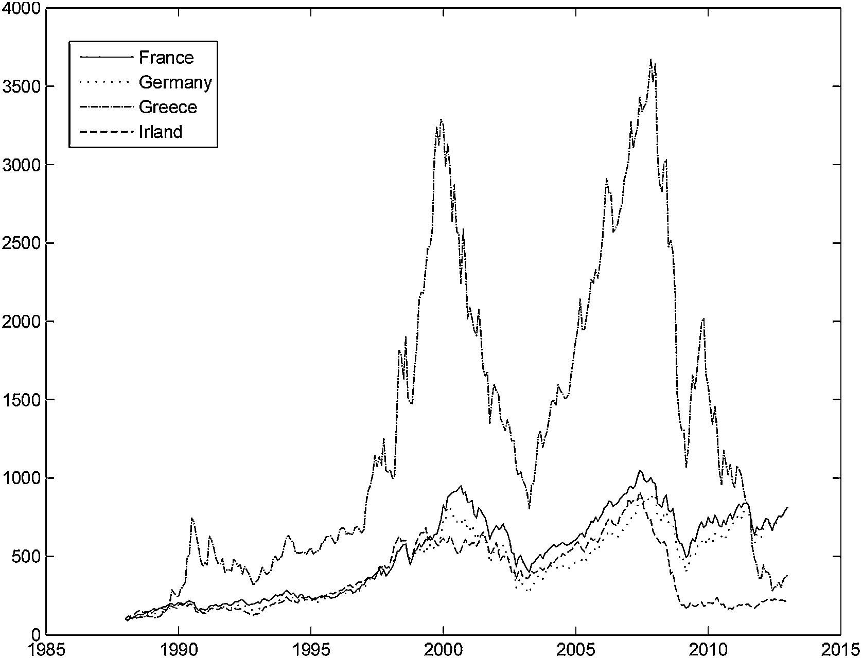
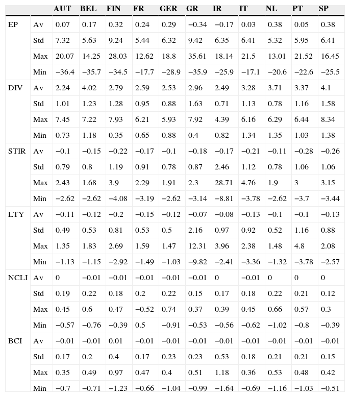
Table 1 presents some descriptive statistics for the country-specific variables. The mean equity premium was highest for Netherlands and Spain, and negative for Greece and Ireland. Even though the equity premia was negative for both Ireland and Greece, the stock market performance was very different in these countries. Fig. 1 shows the total return index evolution for these two countries, and for the core Eurozone countries (France and Germany). It is clear that the Greek stock market presented a stellar performance until the year 2000, and then suffered a large drop in 2002–2003. It then recovered sharply until the advent of the recent financial crisis, and then fell sharply again. By contrast, the evolution of the Irish stock market was much more smooth.
Descriptive statistics for country-specific variables.
| AUT | BEL | FIN | FR | GER | GR | IR | IT | NL | PT | SP | ||
|---|---|---|---|---|---|---|---|---|---|---|---|---|
| EP | Av | 0.07 | 0.17 | 0.32 | 0.24 | 0.29 | −0.34 | −0.17 | 0.03 | 0.38 | 0.05 | 0.38 |
| Std | 7.32 | 5.63 | 9.24 | 5.44 | 6.32 | 9.42 | 6.35 | 6.41 | 5.32 | 5.95 | 6.41 | |
| Max | 20.07 | 14.25 | 28.03 | 12.62 | 18.8 | 35.61 | 18.14 | 21.5 | 13.01 | 21.52 | 16.45 | |
| Min | −36.4 | −35.7 | −34.5 | −17.7 | −28.9 | −35.9 | −25.9 | −17.1 | −20.6 | −22.6 | −25.5 | |
| DIV | Av | 2.24 | 4.02 | 2.79 | 2.59 | 2.53 | 2.96 | 2.49 | 3.28 | 3.71 | 3.37 | 4.1 |
| Std | 1.01 | 1.23 | 1.28 | 0.95 | 0.88 | 1.63 | 0.71 | 1.13 | 0.78 | 1.16 | 1.58 | |
| Max | 7.45 | 7.22 | 7.93 | 6.21 | 5.93 | 7.92 | 4.39 | 6.16 | 6.29 | 6.44 | 8.34 | |
| Min | 0.73 | 1.18 | 0.35 | 0.65 | 0.88 | 0.4 | 0.82 | 1.34 | 1.35 | 1.03 | 1.38 | |
| STIR | Av | −0.1 | −0.15 | −0.22 | −0.17 | −0.1 | −0.18 | −0.17 | −0.21 | −0.11 | −0.28 | −0.26 |
| Std | 0.79 | 0.8 | 1.19 | 0.91 | 0.78 | 0.87 | 2.46 | 1.12 | 0.78 | 1.06 | 1.06 | |
| Max | 2.43 | 1.68 | 3.9 | 2.29 | 1.91 | 2.3 | 28.71 | 4.76 | 1.9 | 3 | 3.15 | |
| Min | −2.62 | −2.62 | −4.08 | −3.19 | −2.62 | −3.14 | −8.81 | −3.78 | −2.62 | −3.7 | −3.44 | |
| LTY | Av | −0.11 | −0.12 | −0.2 | −0.15 | −0.12 | −0.07 | −0.08 | −0.13 | −0.1 | −0.1 | −0.13 |
| Std | 0.49 | 0.53 | 0.81 | 0.53 | 0.5 | 2.16 | 0.97 | 0.92 | 0.52 | 1.16 | 0.88 | |
| Max | 1.35 | 1.83 | 2.69 | 1.59 | 1.47 | 12.31 | 3.96 | 2.38 | 1.48 | 4.8 | 2.08 | |
| Min | −1.13 | −1.15 | −2.92 | −1.49 | −1.03 | −9.82 | −2.41 | −3.36 | −1.32 | −3.78 | −2.57 | |
| NCLI | Av | 0 | −0.01 | −0.01 | −0.01 | −0.01 | −0.01 | 0 | −0.01 | 0 | 0 | 0 |
| Std | 0.19 | 0.22 | 0.18 | 0.2 | 0.22 | 0.15 | 0.17 | 0.18 | 0.22 | 0.21 | 0.12 | |
| Max | 0.45 | 0.6 | 0.47 | −0.52 | 0.74 | 0.37 | 0.39 | 0.45 | 0.66 | 0.57 | 0.3 | |
| Min | −0.57 | −0.76 | −0.39 | 0.5 | −0.91 | −0.53 | −0.56 | −0.62 | −1.02 | −0.8 | −0.39 | |
| BCI | Av | −0.01 | −0.01 | 0.01 | −0.01 | −0.01 | −0.01 | −0.01 | −0.01 | −0.01 | −0.01 | −0.01 |
| Std | 0.17 | 0.2 | 0.4 | 0.17 | 0.23 | 0.23 | 0.53 | 0.18 | 0.21 | 0.21 | 0.15 | |
| Max | 0.35 | 0.49 | 0.97 | 0.47 | 0.4 | 0.51 | 1.18 | 0.36 | 0.53 | 0.48 | 0.42 | |
| Min | −0.7 | −0.71 | −1.23 | −0.66 | −1.04 | −0.99 | −1.64 | −0.69 | −1.16 | −1.03 | −0.51 |
EP – Equity premia, DIV – Dividend yield, STIR – Short-term interest rate less its twelve month moving average, LTY – Long-term bond yield less its twelve month moving average, NCLI – Monthly change in the OECD normalized composite leading indicator, BCI – Monthly change in the OECD business confidence indicator. Av – Average, Std – Standard deviation, Max – Maximum, Min – Minimum. All the values are in percentage points, except for NCLI and BCI.

The average dividend yield over the period considered ranged between a minimum of 2.24% for Austria and a maximum of 4.1% for Spain. Countries that present a larger standard deviation for the equity premium also tend to exhibit a larger standard deviation for the dividend yield.
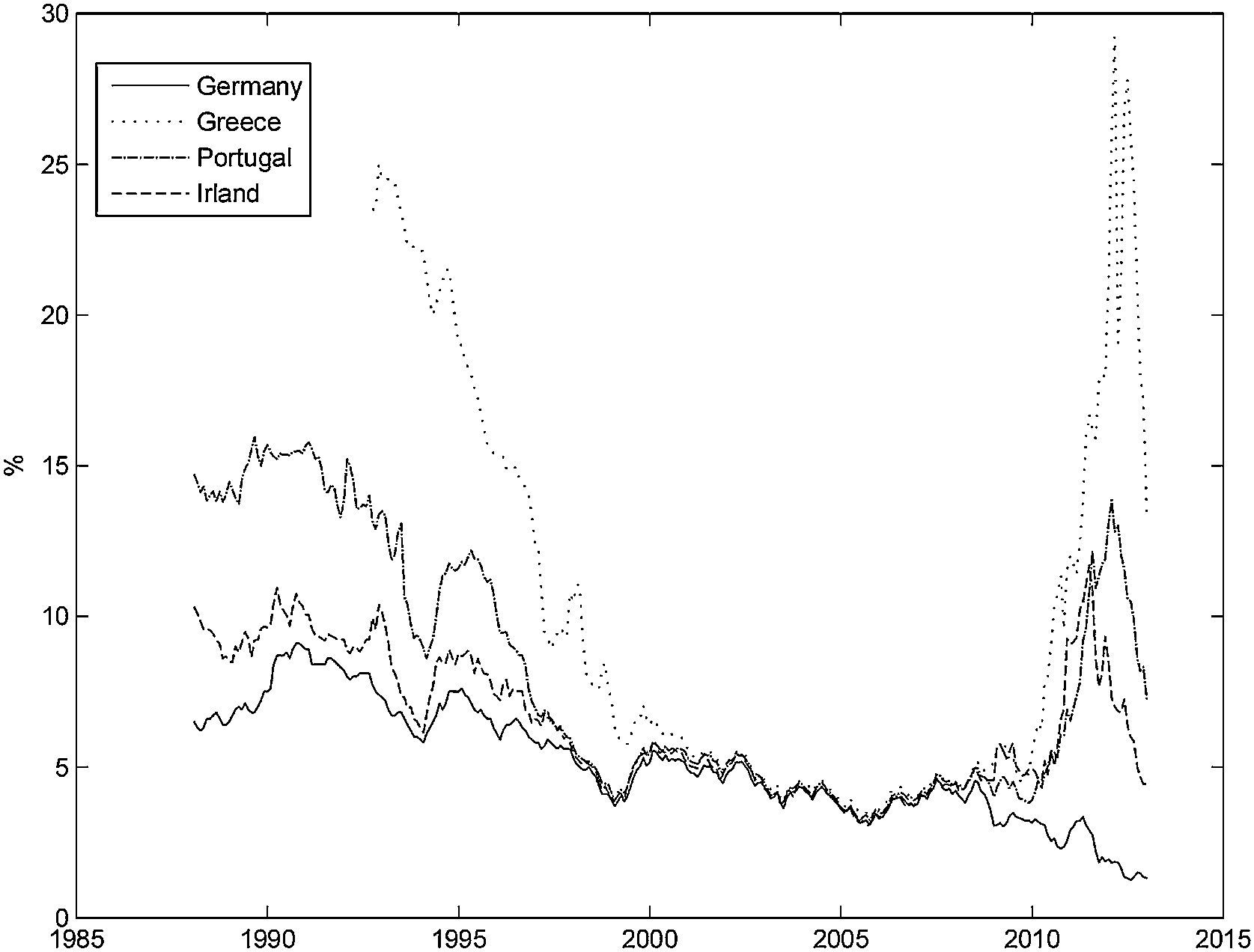
The short-term interest rate and the long-term bond yield presented a downward trend for all the countries over the period considered. The short-term interest rate for Ireland presents the largest standard deviation, due to a sharp interest rate rise in 1992, that was quickly reversed. The long-term bond yield converged across countries until the creation of the Euro, but then it diverged again, following the recent financial crisis, particularly in the peripheral EuroZone countries. Fig. 2 shows the long-term yield evolution for the countries that requested financial assistance following the recent financial crisis (Greece, Ireland and Portugal), and for Germany. It is clear that the long-term yield for Greece, Ireland and Portugal quickly converged toward the German levels before the creation of the Euro. Their spread with respect to the German yield stayed at a low level, until 2008, and then it increased sharply.

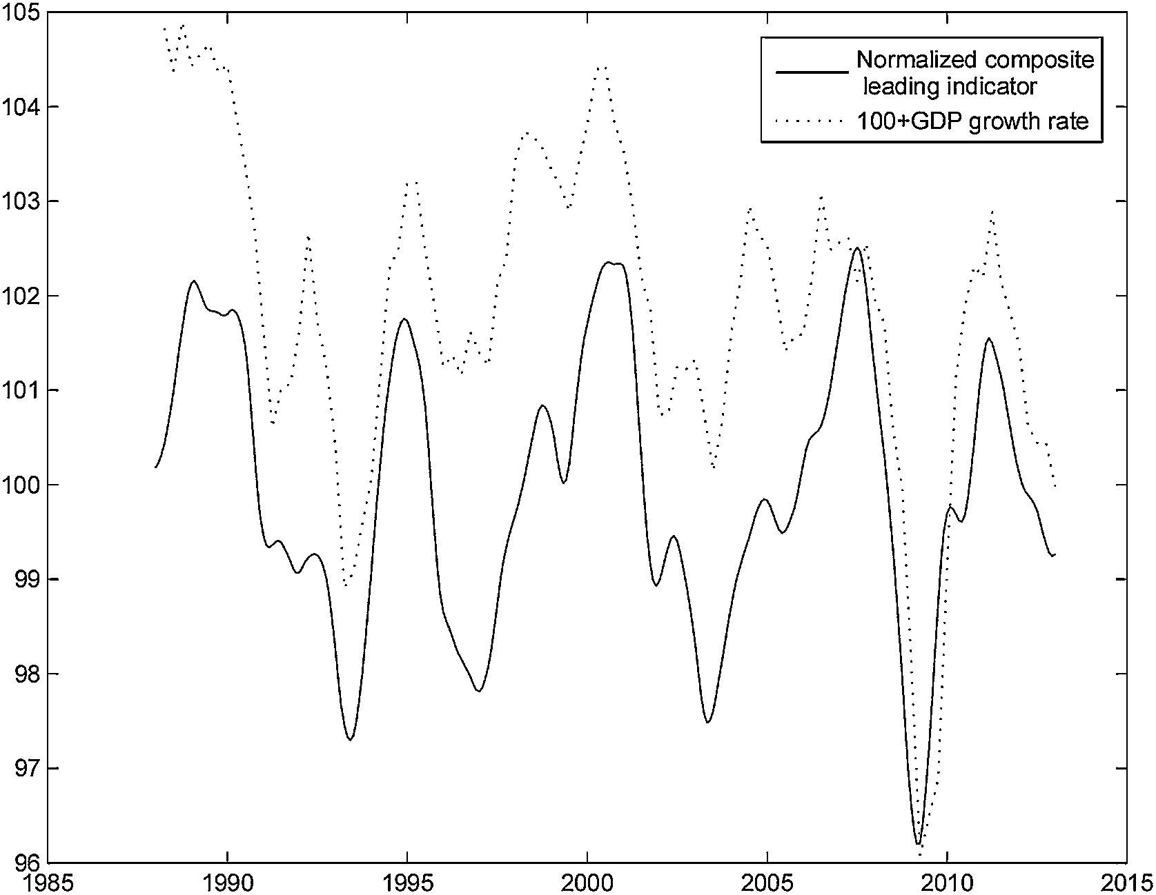
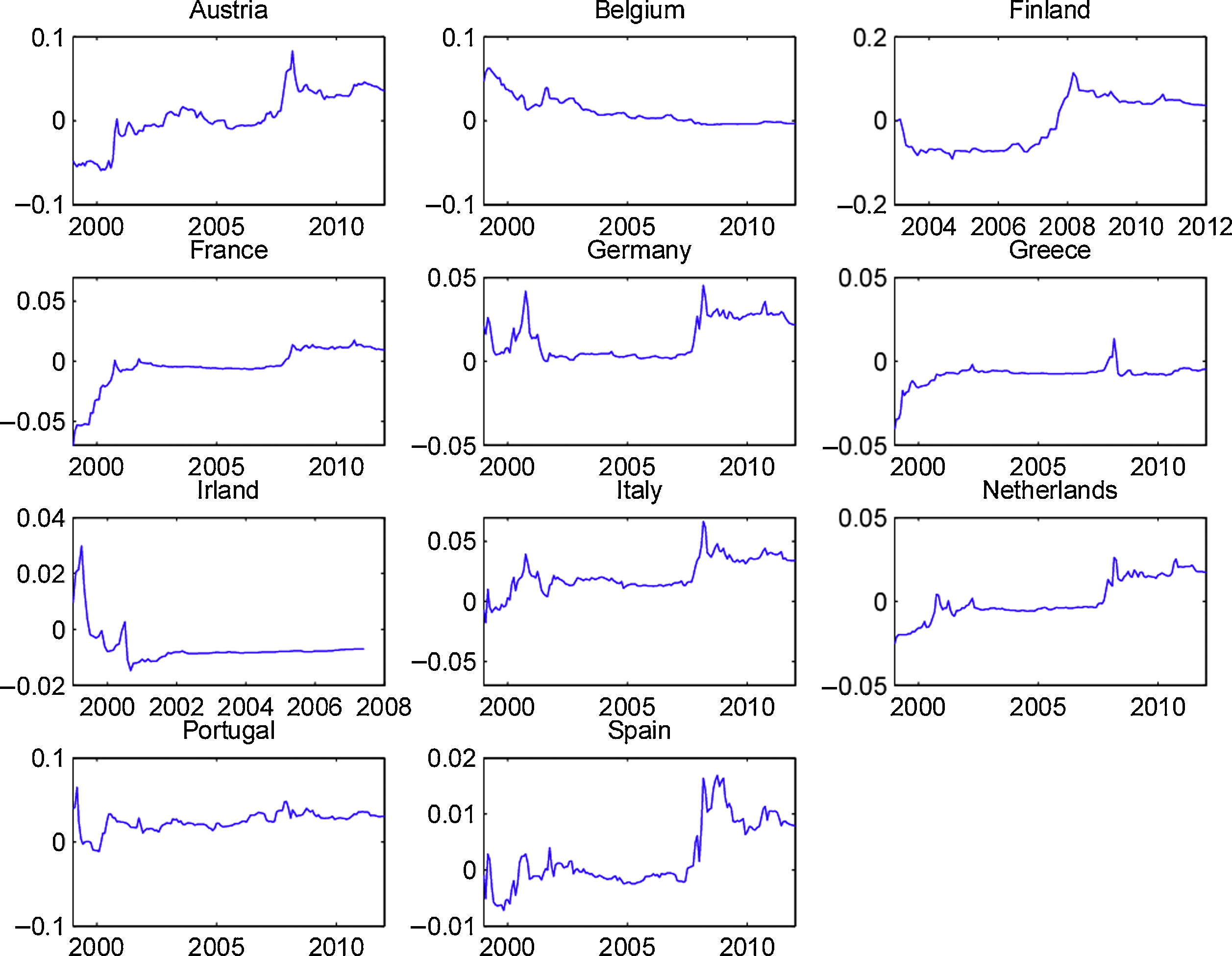
The mean values of the changes in the OECD normalized composite leading indicators and business confidence indicator are close to zero for all the countries, because, over several economic cycles, positive changes tend to alternate with negative changes. Fig. 3 presents the normalized composite leading indicator for France and the change in GDP over the previous year, to which we added 100, in order to make the figure easier to read. It is clear that the leading indicator tends to anticipate changes in the economic cycle. It changes direction before GDP. Even though we used France as an example, the pattern for the other countries is similar.

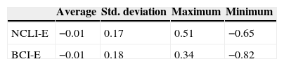
Table 2 presents the descriptive statistics for the EuroZone indicators. Their mean is also close to zero, but their standard deviation is slightly lower than the standard deviations for most country-specific OECD indicators.
3MethodologyAccording to Inoue and Kilian (2005) in-sample test of stock return predictability is more powerful than out-of-sample tests, because the former uses the full sample to fit the models. However, an investor is probably more interested in the out-of-sample performance of the models, which might provide useful information for his investment decisions. Therefore, we have chosen to present both in-sample and out-of-sample tests of stock return predictability.
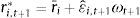
3.1In-sampleWe based our analysis of equity premium predictability on the following regression:
where ri,t+1 is the equity premium, for country i (i=1, …, N), from the end of month t to the end of month t+1, Xi,t is a vector of explanatory variables, for country i, at the end of month t,4 and εi,t+1 is a zero-mean disturbance term for country i. We considered both univariate regressions, in which Xi,t comprises only one explanatory variable, and multivariate regressions. We estimated two kinds of multivariate regressions for each country: in the first one (“kitchen sink”) we included all the country-specific variables, and in the second one (model selection) we selected amongst the 2k-1 models (where k represents the number of country-specific variables), comprising all the possible combinations of explanatory variables, at each time t, the best one according to the Akaike information criterion. All the models were estimated by ordinary least squares, with heteroskedasticity-robust standard errors (White, 1980).
As has been pointed out by Stambaugh (1999), direct inferences, based on the OLS estimates, may produce misleading conclusions. This author has shown that whenever the predictors follow an AR(1) process whose disturbances are negatively correlated with the regression innovations, then the slope coefficient's estimator and the t-statistic are biased upward, which implies that the null hypothesis of no predictability is rejected too often.
In order to circumvent the Stambaugh bias problem, and increase the robustness of our results, we based our inferences on the p-values derived from the wild bootstrap procedure, described in Gonçalves and Kilian (2004) and Rapach et al. (2013). This method generates a set of simulated time series, under the null hypothesis of no predictability, and its implementation requires that we:
- 1.
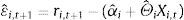
Compute the residuals from the OLS estimates of Eq. (1)
where (αˆi,Θˆi) are the OLS estimates. - 2.
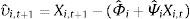
Estimate a VAR(1), for each country and explanatory variable, using Amihud et al. (2009) reduced-bias estimation method
and compute the residuals, using the estimates (Φˆi,Ψˆi): - 3.
Generate a pseudo-sample, under the null hypothesis of no predictability
where r¯i is the sample mean of ri, Xi,1*=Xi,1 and ωt+1 is a draw from the standard normal distribution. We repeat step 3 one thousand times, in order to generate 1000 pseudo-samples. - 4.
Finally, we estimate Eq. (1), for each of the pseudo-samples, and compute the corresponding t-statistics for the slope coefficients, and χ2-statistics in order to test the null hypothesis that no predictor is significant in the multivariate regressions.


The out-of-sample forecast uses only the data available until the time at which the forecast is made. The first prediction period is month 121, that is, we used the first 120 observations to estimate the model parameters, in order to predict the equity premium at month 121
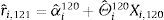
Then, we re-estimated the model using 121 observations, and computed the predicted equity premium at month 122
We repeated this procedure until the end of the sample.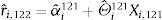
We used several measures that complement one another, in order to evaluate the value of the forecasts. We computed the pseudo R-squared out-of sample to evaluate if the predictions are close to the realized equity premia, in a mean-square sense. The statistical significance of the pseudo R-squared out-of-sample was tested using the MSPE-adjusted statistic. The Pesaran and Timmerman sign test aims to test if the predictors anticipate correctly the direction of stock market changes. Finally, we computed the utility gains that an investor who based his portfolio choice in the predictions would have obtained, in order to test the economic value of the forecasts. A brief description of these tests is presented in the next subsections.
3.2.1Pseudo R2 out-of-sampleThis measure is based on the comparison of the mean-squared prediction error (MSPE) from the model and the MSPE from the historical mean, computed using only the information up to the date at which the forecast is made
where MSPEmod represents the MSPE from the model, and MSPEmean is the MSPE from the historical mean. Note that if the forecast based on the model outperforms the forecast based on the historical mean, in a mean-square sense, then ROOS2 will be positive.3.2.2MSPE-adjusted statistic
This test, proposed by Clark and West (2007), is an approximately normal modified version of McCraken (2007) MSE-F statistic, which is used to test the null hypothesis that the unrestricted model MSPE is equal to the restricted model MSPE, against the one-sided alternative hypothesis that the former MSPE is lower than the later. The most convenient way to implement this test is to compute
where rˆi,tmod is the equity premium prediction for country i, at month t, based on the model, and rˆi,tmean is the equity premium prediction for country i, at month t, based on the historical mean. The MSPE-adjusted statistic is computed by regressing fˆi,t on a constant, and using the resulting t-statistic for a zero coefficient. The null hypothesis of equal predictive ability is rejected, at the 5% confidence level, if the t-statistic exceeds 1.645 (one-sided test).3.2.3Pesaran and Timmermann sign test
The Pesaran and Timmermann (1992) nonparametric sign test is designed to evaluate if the model forecasts have the same sign as the variable that is being predicted. The test is computed as follows:
where T*1/2 is the number of observations in the forecast period, H is the probability of correctly predicting the sign of positive equity premia, F is the probability of incorrectly predicting the sign of negative equity premia, π is the probability that the equity premium is positive, and πˆ is the probability that the predicted equity premium is positive. The PT test is one-sided and asymptotically follows a standard normal distribution.3.2.4Utility gains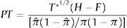
The previous performance evaluation measures are statistical in nature, and do not necessarily bear a direct relation with the benefits of forecasting the equity premium for an investor. In order to assess the economic value of the predictions, we compute the utility gains for a mean-variance investor, who incorporates the models’ predictions in his investment decisions. We assume that the investor can choose between two types of investments, stock market and the riskless asset and, as in Campbell and Thompson (2008), we consider that the fraction of wealth invested in equities can neither exceed 150% nor fall below 0% (no short-selling).
A mean-variance investor from country i, with coefficient of relative risk aversion γ, who forecasts the equity premium using the historical average, will invest a fraction wi,tmean of his wealth in equities, at each month t
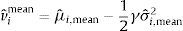
where σˆi,t+12 is the rolling window (60 month) estimate of the variance of stock returns. Over the out-of-sample period, an investor who follows this strategy obtains an average utilitywhere μˆi,mean and σˆi,mean2 represent the sample average and variance, respectively, over the out-of-sample period, for the portfolio formed using only information about the historical mean.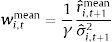
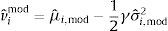
The optimal portfolio weight and the average utility for a country i investor that bases his investment decisions on the predictive model are
where μˆi,mod and σˆi,mod2 are the sample average and variance, respectively, over the out-of sample period, for the portfolio formed using the predictive model.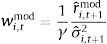
The net average benefit per month for an investor who uses the predictive model is
and can be interpreted as the average monthly fee that an investor from country i would be willing to pay to have access to the model's forecasts.4Results4.1Country-specific predictors4.1.1In-sample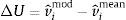
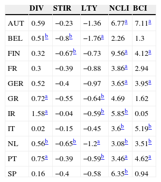
In this subsection, we present the main results of the predictive regressions, in sample, using country-specific data. Table 3 displays the slope coefficients of the univariate regressions, for each country and predictive variable. Most coefficients have the expected sign. The equity premia are positively related with the dividend yields, the changes in the OECD composite leading indicators and business confidence indicators, and negatively related with the short-term interest rates (Greece is the only exception) and the long-term bond yields. We also present the statistical significance of each slope coefficient (one-sided test), computed from the wild bootstrap procedure described above. Analyzing the results by predictor, we conclude that the change in the OECD composite leading indicator has the best performance (significant in 9 countries at the 5% level). The remaining variables also exhibit some explanatory power (between three significant coefficients for the short-term interest rate and six for the change in the OECD business confidence indicator). Note also that, for each country, there is, at least, one significant predictor.
Univariate regressions’ slope coefficients for 11 EuroZone countries (AUT – Austria, BEL – Belgium, FIN – Finland, FR – France, GER – Germany, GR – Greece, IR – Ireland, IT – Italy, NL – Netherlands, PT – Portugal, SP – Spain).
| DIV | STIR | LTY | NCLI | BCI | |
|---|---|---|---|---|---|
| AUT | 0.59 | −0.23 | −1.36 | 6.77a | 7.11a |
| BEL | 0.51b | −0.8b | −1.76a | 2.26 | 1.3 |
| FIN | 0.32 | −0.67b | −0.73 | 9.56a | 4.12a |
| FR | 0.3 | −0.39 | −0.88 | 3.86a | 2.94 |
| GER | 0.52 | −0.4 | −0.97 | 3.65a | 3.95a |
| GR | 0.72a | −0.55 | −0.64b | 4.69 | 1.62 |
| IR | 1.58a | −0.04 | −0.59b | 5.85b | 0.05 |
| IT | 0.02 | −0.15 | −0.45 | 3.6b | 5.19b |
| NL | 0.56b | −0.65b | −1.2a | 3.08b | 3.51b |
| PT | 0.75a | −0.39 | −0.59b | 3.46a | 4.62a |
| SP | 0.16 | −0.4 | −0.58 | 6.35b | 0.94 |
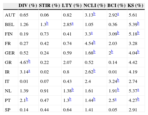
Columns 1–5 of Table 4 report the in-sample R-squared values for the univariate regressions, whereas the last column presents the in-sample R-squared for the “kitchen sink” model (the model that includes all the country-specific predictors). Amongst the univariate regressions, the OECD predictors exhibit the best performance, with 6 significant R-squared. The dividend yield and the long-term bond yield are significant for 3 countries each, and the short-term interest rate is significant only for Belgium. Regarding the “kitchen sink” model, there are 5 significant R-squared. This kind of model usually fits the data better than univariate models in-sample, but its out-of-sample performance is often disappointing, due to data overfitting (see, for example, Goyal and Welch, 2008).
In-sample R-squared for 11 EuroZone countries (AUT – Austria, BEL – Belgium, FIN – Finland, FR – France, GER – Germany, GR – Greece, IR – Ireland, IT – Italy, NL – Netherlands, PT – Portugal, SP – Spain) and 6 models (DIV – dividend yield, STIR – short-term interest rate, LTY – long-term yield, NCLI – change in the OECD composite leading indicator, BCI – change in the business confidence indicator, KS – “kitchen sink”).
| DIV (%) | STIR (%) | LTY (%) | NCLI (%) | BCI (%) | KS (%) | |
|---|---|---|---|---|---|---|
| AUT | 0.65 | 0.06 | 0.82 | 3.13b | 2.92a | 5.61 |
| BEL | 1.26 | 1.3b | 2.85a | 1.05 | 0.36 | 5.39b |
| FIN | 0.19 | 0.73 | 0.41 | 3.3a | 3.09b | 5.18b |
| FR | 0.27 | 0.42 | 0.74 | 4.54b | 2.03 | 3.28 |
| GER | 0.52 | 0.24 | 0.59 | 1.68b | 2b | 4.04b |
| GR | 4.67b | 0.22 | 2.07 | 0.52 | 0.14 | 4.42 |
| IR | 3.14a | 0.02 | 0.8 | 2.62b | 0.01 | 4.19 |
| IT | 0.01 | 0.07 | 0.43 | 2.4 | 3.24b | 2.74 |
| NL | 1.39 | 0.91 | 1.38b | 1.61 | 1.91b | 5.37a |
| PT | 2.1b | 0.47 | 1.3b | 1.44b | 2.5a | 4.27b |
| SP | 0.14 | 0.44 | 0.64 | 1.41 | 0.05 | 2.91 |
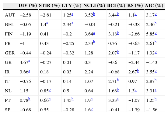
In this subsection we present the out-of-sample statistical and economic performance measures, for both the univariate and the multivariate models. Table 5 displays the R-squared out-of-sample for the univariate models (columns 1–5), the kitchen sink model (column 6), and the best model selected according to the Akaike information criterion (column 7). Amongst the univariate models, the best is the one based on the OECD business confidence indicator, with 6 significant R-squared. The change in OECD normalized composite leading indicator also exhibits a good out-of-sample predictive ability (6 significant R-squared and 1 negative). The results for the remaining variables provide mixed evidence of predictability, with some significant R-squares, but some negative ones also.
Out-of sample R-squared for 11 EuroZone countries (AUT – Austria, BEL – Belgium, FIN – Finland, FR – France, GER – Germany, GR – Greece, IR – Ireland, IT – Italy, NL – Netherlands, PT – Portugal, SP – Spain) and 7 models (DIV – dividend yield, STIR – short-term interest rate, LTY – long-term yield, NCLI – change in the OECD composite leading indicator, BCI – change in the business confidence indicator, KS – “kitchen sink”, AIC – Akaike information criterion).
| DIV (%) | STIR (%) | LTY (%) | NCLI (%) | BCI (%) | KS (%) | AIC (%) | |
|---|---|---|---|---|---|---|---|
| AUT | −2.58 | −2.61 | 1.25a | 3.52b | 3.44b | 1.1b | 3.17b |
| BEL | −0.05 | 1.4a | 2.34a | −0.01 | −0.21 | −0.38 | 2.46b |
| FIN | −1.19 | 0.41 | −0.2 | 3.64a | 3.18b | −2.66 | 5.85b |
| FR | −1 | 0.43 | −0.25 | 2.33b | 0.76 | −0.65 | 2.61b |
| GER | −0.44 | −0.24 | −0.32 | 1.28 | 2.07b | −1.17 | 1.32b |
| GR | 4.67a | −0.27 | 0.01 | 0.3 | −0.6 | −2.44 | −1.43 |
| IR | 3.66a | 0.18 | 0.03 | 2.24 | −0.68 | 2.67b | 3.55b |
| IT | −0.75 | −0.17 | 0.14 | 1.07 | 2.71b | 0.97 | 2.87b |
| NL | 1.15 | 0.85b | 0.5 | 0.64 | 1.68b | 1.3b | 3.31a |
| PT | 0.78b | 0.66b | 1.45b | 1.9b | 3.33a | −1.07 | 1.25b |
| SP | −0.68 | 0.55 | −0.28 | 1.6b | −0.41 | −1.39 | −1.56 |
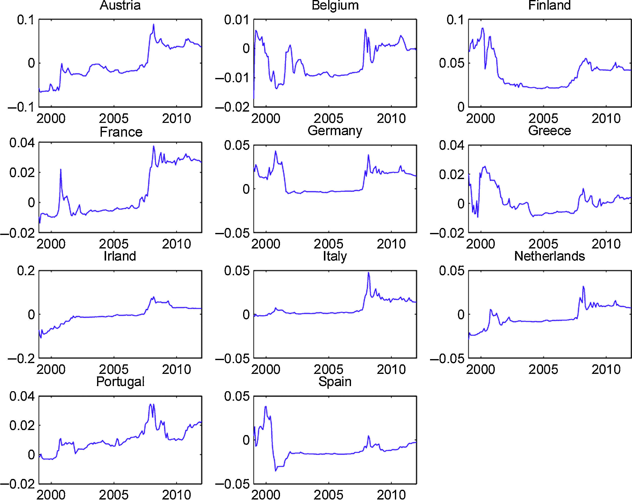
To our knowledge, the OECD predictors, which present a good out-of-sample performance, have not previously been used in the equity premium forecast literature. Therefore, it is interesting to analyze if their forecasting ability is restricted to some particular part of the sample. In order to accomplish this objective, we show, in Figs. 4 and 5, the cumulative out-of-sample R-squared, for these variables, in every country. That is, for each month, we compute the difference between the cumulative mean forecast error from the forecasts based on the historical mean, and the cumulative mean forecast error from the predictive model, and then we divide this difference by the cumulative mean forecast error from the forecasts based on the historical mean. The model based on the predictive variables outperforms (underperforms) the historical average in periods at which the line in the figure increases (decreases).


Fig. 4 presents the graphs for the OECD normalized composite leading indicator. It is clear that, for most countries, this indicator presented a very good performance during the early months of the recent financial crisis. Although we cannot draw definitive conclusions from this relatively short out-of-sample period (roughly 15 years), this variable seems to be a promising indicator of the stock market downturn at the beginning of economic contractions. Fig. 5 displays the graphs for the OECD business confidence indicator. Even though the OECD business confidence indicator has some ability to predict stock market contractions, it seems weaker than the one for the OECD composite leading indicator.
Regarding the multivariate models, the model chosen according to the Akaike information criterion clearly exhibits the best overall performance, with nine significant R-squared, and the “kitchen sink” model generally presents a poor predictive ability, probably due to data overfitting.
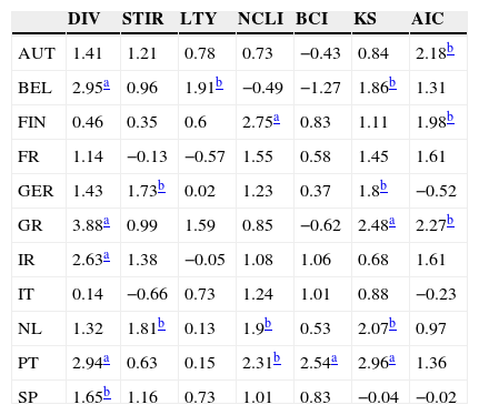
Table 6 displays the results of the Pesaran and Timmermann (1992) sign test. Curiously, multivariate models perform better according to this criterion than univariate ones. In particular, the “kitchen sink” model, that has a modest performance, when measured by the R-squared out-of-sample, exhibits a good ability to predict the sign of the equity premia (almost all the test results are positive, and five are significant at the 5% level). Amongst the univariate models, the dividend yield is the best predictor followed by the OECD normalized composite leading indicator. Overall, there is a mild degree of predictability of the equity premia signs.
Pesaran and Timmermann sign test for 11 EuroZone countries (AUT – Austria, BEL – Belgium, FIN – Finland, FR – France, GER – Germany, GR – Greece, IR – Ireland, IT – Italy, NL – Netherlands, PT – Portugal, SP – Spain) and 7 models (DIV – dividend yield, STIR – short-term interest rate, LTY – long-term yield, NCLI – change in the OECD composite leading indicator, BCI – change in the business confidence indicator, KS – “kitchen sink”, AIC – Akaike information criterion).
| DIV | STIR | LTY | NCLI | BCI | KS | AIC | |
|---|---|---|---|---|---|---|---|
| AUT | 1.41 | 1.21 | 0.78 | 0.73 | −0.43 | 0.84 | 2.18b |
| BEL | 2.95a | 0.96 | 1.91b | −0.49 | −1.27 | 1.86b | 1.31 |
| FIN | 0.46 | 0.35 | 0.6 | 2.75a | 0.83 | 1.11 | 1.98b |
| FR | 1.14 | −0.13 | −0.57 | 1.55 | 0.58 | 1.45 | 1.61 |
| GER | 1.43 | 1.73b | 0.02 | 1.23 | 0.37 | 1.8b | −0.52 |
| GR | 3.88a | 0.99 | 1.59 | 0.85 | −0.62 | 2.48a | 2.27b |
| IR | 2.63a | 1.38 | −0.05 | 1.08 | 1.06 | 0.68 | 1.61 |
| IT | 0.14 | −0.66 | 0.73 | 1.24 | 1.01 | 0.88 | −0.23 |
| NL | 1.32 | 1.81b | 0.13 | 1.9b | 0.53 | 2.07b | 0.97 |
| PT | 2.94a | 0.63 | 0.15 | 2.31b | 2.54a | 2.96a | 1.36 |
| SP | 1.65b | 1.16 | 0.73 | 1.01 | 0.83 | −0.04 | −0.02 |
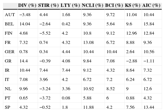
Table 7 presents the annualized utility gains, which could have been obtained by a mean-variance investor that incorporates the models’ forecasts in his investment decisions. Most utility gains are positive and some are quite high, which means that, generally, these predictors provide economically significant benefits. For three of the predictive models (long-term bond yield, OECD normalized composite leading indicator, OECD business confidence indicator) the utility gains are positive for every country, and some of these gains are considerable, exceeding 10%. Note also that the strategy that selects the best model according to the Akaike information criterion provides positive utility gains for every country except Greece.
Annualized utility gains for 11 EuroZone countries (AUT – Austria, BEL – Belgium, FIN – Finland, FR – France, GER – Germany, GR – Greece, IR – Ireland, IT – Italy, NL – Netherlands, PT – Portugal, SP – Spain) and 7 models (DIV – dividend yield, STIR – short-term interest rate, LTY – long-term yield, NCLI – change in the OECD composite leading indicator, BCI – change in the business confidence indicator, KS – “kitchen sink”, AIC – Akaike information criterion).
| DIV (%) | STIR (%) | LTY (%) | NCLI (%) | BCI (%) | KS (%) | AIC (%) | |
|---|---|---|---|---|---|---|---|
| AUT | −3.48 | 4.44 | 1.68 | 9.36 | 9.72 | 11.04 | 10.44 |
| BEL | 14.04 | −2.64 | 0.42 | 9.36 | 5.64 | 9.6 | 15.84 |
| FIN | 4.68 | −5.52 | 4.2 | 10.8 | 9.12 | 12.96 | 12.84 |
| FR | 7.32 | 0.74 | 4.32 | 13.08 | 6.72 | 8.88 | 9.36 |
| GER | 0.78 | 0.34 | 4.44 | 10.44 | 10.44 | 2.64 | 10.56 |
| GR | 14.4 | −0.39 | 4.08 | 9.84 | 7.08 | −2.88 | −1.11 |
| IR | 10.44 | 7.44 | 7.44 | 9.12 | 4.32 | 8.64 | 7.32 |
| IT | 7.08 | 3.96 | 4.2 | 6.72 | 7.2 | 6.24 | 6.72 |
| NL | 9.96 | −3.24 | 3.36 | 10.92 | 8.52 | 9 | 12.6 |
| PT | 0.65 | −3.72 | 0.08 | 5.88 | 6 | 0.88 | 4.32 |
| SP | 4.32 | −0.52 | 1.8 | 11.88 | 4.2 | 7.56 | 13.44 |
In this subsection we present the in-sample and out-of-sample performance measures of the explanatory regressions that use EuroZone variables. We considered both univariate regressions and multivariate regressions, where both EuroZone predictors were included simultaneously.
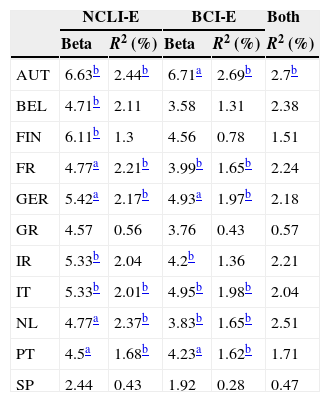
From Table 8, we see that all the slope coefficients are positive, as expected, which implies that an improvement in the EuroZone economic indicators has a positive impact on stock markets’ performances. There is a considerable number of significant in-sample R-squared for the univariate regression (6 significant R-squared, at the 5% confidence level), mainly in the core EuroZone countries. This result is not surprising, given that these countries’ stock markets include a substantial number of multinational companies, whose performance depends on the economic health of the EuroZone as a whole. Regarding the regressions that include both predictors, there is only one significant R-squared. Changes in the EuroZone composite leading indicator and business confidence indicator are highly correlated, which decreases the value added of using both predictors in the same regression.
Univariate regressions’ slope coefficients and in-sample R-squared for 11 Eurozone countries (AUT – Austria, BEL – Belgium, FIN – Finland, FR – France, GER – Germany, GR – Greece, IR – Ireland, IT – Italy, NL – Netherlands, PT – Portugal, SP – Spain).
| NCLI-E | BCI-E | Both | |||
|---|---|---|---|---|---|
| Beta | R2 (%) | Beta | R2 (%) | R2 (%) | |
| AUT | 6.63b | 2.44b | 6.71a | 2.69b | 2.7b |
| BEL | 4.71b | 2.11 | 3.58 | 1.31 | 2.38 |
| FIN | 6.11b | 1.3 | 4.56 | 0.78 | 1.51 |
| FR | 4.77a | 2.21b | 3.99b | 1.65b | 2.24 |
| GER | 5.42a | 2.17b | 4.93a | 1.97b | 2.18 |
| GR | 4.57 | 0.56 | 3.76 | 0.43 | 0.57 |
| IR | 5.33b | 2.04 | 4.2b | 1.36 | 2.21 |
| IT | 5.33b | 2.01b | 4.95b | 1.98b | 2.04 |
| NL | 4.77a | 2.37b | 3.83b | 1.65b | 2.51 |
| PT | 4.5a | 1.68b | 4.23a | 1.62b | 1.71 |
| SP | 2.44 | 0.43 | 1.92 | 0.28 | 0.47 |
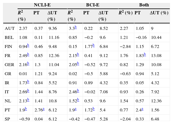
Table 9 presents the out-of-sample results for the EuroZone predictors. Amongst the univariate regressions, more than half of the R-squared are significant. Note that there is a high degree of consistency between the in-sample and out-of-sample results. That is, most of the countries with significant R-squared in-sample have also significant out-of-sample R-squared. For the model that uses both variables, there is no evidence of out-of-sample predictive ability, based on the R-squared out-of-sample. Probably, the fact that the explanatory variables are highly positive correlated renders the estimated parameters unstable.
Out-of-sample R-squared, Pesaran and Timmerman sign test and utility gains for 11 Eurozone countries (AUT – Austria, BEL – Belgium, FIN – Finland, FR – France, GER – Germany, GR – Greece, IR – Ireland, IT – Italy, NL – Netherlands, PT – Portugal, SP – Spain).
| NCLI-E | BCI-E | Both | |||||||
|---|---|---|---|---|---|---|---|---|---|
| R2 (%) | PT | ΔUT (%) | R2 (%) | PT | ΔUT (%) | R2 (%) | PT | ΔUT (%) | |
| AUT | 2.37 | 0.37 | 9.36 | 3.3b | 0.22 | 8.52 | 2.27 | 1.05 | 9 |
| BEL | 1.08 | 0.11 | 11.16 | 0.85 | −0.2 | 9.6 | 1.21 | −0.16 | 10.44 |
| FIN | 0.94b | 0.46 | 9.48 | 0.15 | 1.77b | 6.84 | −2.84 | 1.15 | 6.72 |
| FR | 2.49b | 0.85 | 12.36 | 2.15b | 0.41 | 9.12 | 1.76 | 1.83b | 13.08 |
| GER | 2.16b | 1.3 | 11.04 | 2.05b | −0.52 | 9.72 | 0.82 | 1.29 | 10.08 |
| GR | 0.01 | 1.21 | 9.24 | 0.02 | −0.5 | 5.88 | −0.63 | 0.94 | 5.12 |
| IR | 1.73b | 0.84 | 5.52 | 0.91 | 0.89 | 4.32 | 0.35 | 0.05 | 4.32 |
| IT | 2.69b | 1.44 | 8.76 | 2.46b | −0.02 | 7.08 | 0.93 | 0.26 | 7.92 |
| NL | 2.13b | 1.41 | 10.8 | 1.52b | 0.53 | 9.6 | 1.54 | 0.57 | 12.36 |
| PT | 1.9b | 2.76a | 6.12 | 1.9a | 1.72b | 5.4 | 0.77 | 2.4a | 1.56 |
| SP | −0.59 | 0.04 | 6.12 | −0.42 | −0.47 | 5.28 | −2.04 | 0.33 | 6.48 |
The results of the Pesaran and Timmermann sign test reveal that there is weak evidence of equity premia sign predictability. There is only one significant test value for the composite leading indicator model, and two for the models based on the business confidence indicator and on both predictors.
Columns 3, 6 and 9 exhibit the utility gains for a mean-variance investor. Even though the statistical evidence of predictability is mixed, an investor could have obtained substantial economic benefits, if he had used these predictive models. Utility gains are positive in almost every country, and often exceed 5% annually. We may conclude that the correlation between the statistical and economic performance measures is far from perfect.
5ConclusionsIn this paper we have shown that there is evidence of both in-sample and out-of-sample equity premia predictability, in most EuroZone countries. Amongst the univariate regressions, the new variable that we have proposed – the change in the OECD normalized composite leading indicator – exhibits the best overall performance. The performance of the strategy that selects the best model according to Akaike information criterion, using only information that is available up to the time at which the forecast is made, is very consistent, and delivers substantial economic benefits.
We have also shown that, for the vast majority of the countries and models considered, a mean-variance investor could have obtained utility gains, if he had based his decisions on the models’ forecasts. Furthermore, we found that there is no evidence of a direct relation between the statistical performance and the economic benefits of the predictions.
We think that the evidence of predictability of stock market contractions, based on the OECD indicators deserves a closer look, in order to evaluate if it is restricted to this particular time period and group of countries, or if it generalizes to a wider group of countries and time span.
For Greece and Italy we have used the 3-month treasury-bill rate, because we could not obtain money market data for the entire period.
Long-term bond yield data for Greece begins in September 1992.
Data for Finland begins in September 1992, and for Ireland ends in April 2008.
We used month t−2 data for the OECD normalized composite leading indicator, and month t−1 for the OECD business confidence indicator, because these variables are only available with a 2-month and 1-month lags, respectively.

