


This research intends to find out any development of a robust multi-objective for lead time optimal control problem in a multi-stage assembly system model. Assembly system modeling is possible by the help of the open queue network. A working station includes one or infinite servers and just manufacturing or assembly operations are performed therein. Each part has a separate entry process and independent of each other. It is completely based upon Poisson process.Serving Lead Time of Stations are also independent of each other and therefore exponential distribution of each parameter is controllable. All stations have bounded uncertain unrecyclable wastes which are completely independent in compliance with Erlang distribution. Uncertainty in the problem parameters has been suggested as robust multi-objective optimal control model in which we have three incompatible target functions including cyclic operation cost minimization, average lead time minimization and lead time variance. Finally, target progress method has been applied in order to achieve serving optimal speeds and solve discrete time of the main problem approximately. The proposed model could present a suitable solution even for the same problem as mentioned in other related papers along with some considerable results in parameter uncertainty conditions.
Optimization of the problems which are related to queue system is very complex. In literature, there are many problems which are related to queue systems (Smith et al, 1988). Following goals of this paper are: production, programming, improving throughput, deceasing sojourn time and the average number of the client in the system. Controlling servicing speed in each node of the system studied by Jackson package. Schechner et.al (1989) considered maintenance & operation costs. They assumed that costs are functions of the activity frequency which are performed on a node. Tseng and Hsiao (1995) studied optimal control of a queue system input with two stations under constraint of time delay in system in order to maximize throughput in the system. Kerbache and Smith (2000) studied optimal routing and positioning problems from the point of view of system optimization. Baldoquin et.al (2014) and Chen et al (2014) studied a new model for controlling and optimizing servicing speeds and speeds of entry to servicing stations. They intended to optimize waiting length of the system route and total operational costs of their service stations in each period. In all studies performed so far, hypothesis of model parameters certainty were considered as a main hypothesis while many optimization problems were facing with the uncertainty of the parameters. For example, actual demand of products, financial return, required material and other sources are not known in the supply chain at the time of critical decision making. Input parameters of each server, in queue system optimization problems, may face with uncertainty. The optimal answer obtained from the made models may not be optimal or justified due to violation of some constraints as soon as the parameters take any values other than nominal value.
This may result in a natural question in designing of approaches for finding the optimal answer which is safe against the uncertainty of the parameters. They are called Robust Answers. In order to explain the importance of the most robust answer in applications, we refer to a case study which was done by Ben-Tal and Nemirovski (2000) on linear optimization through Net lib.
We can’t neglect that negligible uncertainty in parameters can make optimal normal answer meaningless from the applied point of view In applications of linear programming.
In classic methods, sensitivity analysis and stochastic programming are used in order to consider the uncertainty of the parameters. In the first approach, analyst neglects any effects of parameter uncertainty on the model and uses sensitivity analysis in order to confirm the obtained answers. Parameter Sensitivity Analysis is really a tool for analyzing good answers and we can’t apply it for production of robust answers. In addition, it is not practical to do sensitivity analysis on the models with many uncertain parameters.
Dantzing (1998) has defined stochastic programming as an approach for modeling uncertainty of the parameters. This approach assumed scenarios with different probabilities of occurrence of parameters. In this approach, justifiability of the answer is expressed by the use of chance constraints. There are three main problems for this approach as follows: A-It is difficult to recognize accurate distribution of uncertain parameters and finally quantify the scenarios which are obtained from the concerned distributions, B- Chance constraints exclude convexity of the main problem and increase the complexity, C- Dimensions of the obtained optimization model may be increased astronomically in parallel with the increase of the number of scenarios which causes major calculation challenges.
Robust optimization is another approach which has been introduced for confronting with uncertainty of parameters. In this approach, we have to seek for near optimal answers. On the other hand, we ensure justifiability of the answer by decreasing optimization of the target function. In case of uncertainty in target function coefficients, we should search to find the answer which is better than initial ones with high probability of changing target function.
This article presents an approximate model for controlling and optimizing servicing speed (capacity) in each node in the multiphase assembly system and on the basis of the goals of Baldoquin et.al (2014).
2Multiphase dynamic assembly systemsA multiphase dynamic assembly system can be modeled as an open queue system. A servicing station is embedded in each node and is regarded as an assembly or production operation. The following hypotheses are considered:
Each separate part of the product enters a production system under Poisson process with parameter of λ. Just one product is produced. Servicing station is regarded as a production station with more than an input edge as a production station. A servicing station with more than one input edge is regarded as an assembly station. Each party enters into production station after entering the system to perform production operations on it. If another part is being produced, the new part will be in queue. After completion of process in production station, a part which enters into another station would be exposed to other operations. After production of each part, the concerned part is assembled with other parts in assembly station. The product is completed in end node and leaves the system. Each part has some specifications which are statistically independent of the other parts. Each servicing station comprises one or infinite number of servers. Operation time in servicing stations follows an exponential distribution and is independent of the previous operation time. There is no pause in operations due to failure, repair or other cases. Servicing rule is based on FIFO method. Capacity of queue of all stations is infinite. Transportation times between servicing stations are independent random variables with Erlang distributions. There is a queue system in a stable state. The capacity of the station is controlled by servicing speed of concerned device. Servicing speeds are stepwise variables. Operational costs of a servicing station in each period are ascending functions of servicing speed of that station. Thre are totally two service stations in a queue system nodes. After completion of assembly operations, the server starts the next assembly operation in case of at least one unit item of each part. Assembly station of a queue system is multiple input and its specific characteristic is a cluster servicing in which each cluster includes one unit of a part. Harrison (1973) and Ascencio et.al (2014) showed that it is impossible to create a synchronization analytic method and adjustment of unreported input flows in order to find distribution of lead time in the multiphase assembly system. Therefore, analysts use lead time distribution estimation.
With regard to hypothesis of the model, any entrance to the production stations which are prior to assembly station has a Poisson model with parameter λ. This indicates that entrance of parts to each assembly node is a Poisson process with speed λ. Both nodes in queue system are related to multiphase dynamic assembly system. It is like a tree and waiting times are independent in servicing stations. (Lemoine, 1979)
3Analyzing the longest route in queue systemsThe most important phases of the longest route analysis of queue systems include:
Phase 1. Determining density function of waiting time (including operating time and queue waiting time) in each servicing station. If servicing station has only one machine, the spent time is similar to the system.If servicing station m has only one machine, the spent time is similar to the m/m/1 system.

Where μm and λ are entry rates and the servicing rate in queue system. Therefore, waiting time distribution in mth servicing station is exponential distribution with parameter of (μm-λ). If there is an infinite machine in servicing station, spent time in this M /M / ∞ system will follow an exponential distribution with parameter of μm because there is no queue.
Phase 2. By converting each node which includes servicing station to stochastic edge such as queue system to equivalent stochastic network, length of each edge equals to the time spent in the related servicing station. For more details, refer to Baldoquin et.al (2014). After conversion of all nodes of the stochastic edges, queue system has been converted to equivalent stochastic network.
Phase 3. In this phase, Kalkarni et al. specified the longer route distribution function which has been obtained by the stochastic network. Assume G = (V,A) as a stochastic network in which stands for a set of nodes and A is edged or production operation of the assembly dynamic system after transformation. Starting and terminating nodes are shown with s and t. Length of the edge a in which a ∈ A is a stochastic variable with exponential distribution and parameter λa. For a ∈ A, a(α) consider stochastic variable as the first node of edge a and β(a)as the last node of the edge a. Azaron and Modarres (2005) mentioned the following definitions used in present article:
Definition 1. are sets of input and output edges of node u and are defined as follows:


Definition 2. If s ∈ X, X ⊂ A and t ∈ Xc and where Xc complements set, then, cut (s,t) is defined as follows:

(s,t) is a uniformly directed cut(UDC) if (X, X―) is empty.
Definition 3. If D=E∪F is a UDC of the network, we consider it as an acceptable distance. If we have Iβa⊄FF or each a ∈ F.
Definition 4. Each one of the operations at time t can be dormant or idol in one of the active states which is defined as follows:
Active: Any operations which are being executed at time t.
Dormant: Operations at time t which have been completed, but there is an unfinished operation in it.
Idol: An operation at time t, which is neither active nor dormant.
The set of active and dormant states are shown with Y(t) and Z(t) and X(t) = (Y(t),Z(t)). Now, if S stands for all cuts of the network which have acceptance distance, we can consider s―=S∪ϕ,ϕ where X(ϕ,ϕ) indicates to Z(t) = ϕ, Y(t) = ϕ. It means that all operations at time t are idol and therefore, end product finished at time t leaves the system.
We can prove that {X(t),t ≥ 0} is a Markov process in state space of S― with continuous time. Members of transient matrix in this Markov process which is shown with Q = [q{(E, F), (E', F')}] are UDF of active and dormant operations which have been introduced by Kulkarni, and Adlakha (1986) are as follows:
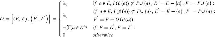
{X(t), ≥ 0} is a finite –state absorbing, continuous Time Markov process and because q{(ϕ,ϕ),(ϕ,ϕ)}=0 is an absorbing state, other states are clearly transient. In addition, we number states S in such a manner that matrix Q is converted to a higher triangle matrix.
It is assumed that these states are numbered as 1,2, ...,N in which N equals to the total number of S― The first state is initial which is shown with X(t) = (O(s),ϕ) and state N is absorbing which is shown with X(t) = (ϕ,ϕ).
Assume that T indicates the longest route in the network with lead time.
It is clear that T=mint>0:Xt=NX0=1
Therefore, T is the time which takes for {X(t),t ≥ 0}to be absorbed by the last phase which has started with 1.
In order to calculate F(t) = P{T ≤ t}or lead distribution function, we can apply backward the Chapman -Kolmongroff relations. In this regard, if Pi(t) is defined as follows:

We will have F(t) = P1(t)
Yinan et.al (2014) presented a differential equation for the vector:
Pt=P1t,P2t,...PNtT as follows:
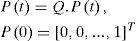
The relations introduced in section 3 are used for constructing an optimization model in the next section.
4Multi-objective lead time control problemIn this section, an analytic model is used for optimal control of servicing the speed in servicing stations. We can increase speed of servicing in production & assembly stations. In this case, average lead time will be shortened accordingly. But this may increase operational costs in each period.
As a result of a suitable tradeoff between average lead time and costs, it is necessary to consider lead time variance because when we concentrate on average lead time, servicing speeds may not be optimal.
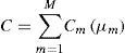
In order to achieve the mentioned goal, a multi-objective problem has been presented by Chen et al (2014) in which three objectives include minimization of total operational costs of the system in each period and minimization of average lead time. The operational cost of ith working station in each period has been regarded as ascending function Cm(μm) where μm is servicing speed of that station. Therefore, C or total operational costs of the system are calculated in each period:
Dalfard et.al (2011) focused on the case in which production capacity is provided for discrete choices. For example, when some machines or workers or one working shift is added, the capacity is controlled with servicing speed in each node. Therefore, servicing speed should be selected among a series of related discrete choices.
With regard to Si as a series of choices for ith servicing speed Cm(μm) constant values are not allocated to transient matrix elements but it is a function of control vectors μ=μ1,μ2,...,μmT. For this reason, nonlinear dynamic model has been suggested as follows:
With regard to Si as a series of choices for ith servicing speed Cm(μm) constant values are not allocated to transient matrix elements but it is a function of control vectors μ=μ1,μ2,...,μmT. For this reason, nonlinear dynamic model has been suggested as follows:
In case B sets of nodes, including servicing stations M /M / 1 and C is set of nodes, including servicing of M /M / ∞, the following relations are used in order to sustain the system:
Such a structure is not available in mathematical programming. Therefore, the following relations are used in defining a multi-objective problem as substitute of the relations:
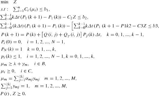
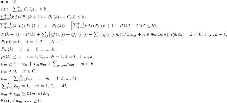
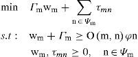
With regard to the relation (11) with help of goal attainment method, multi-objective lead time control model has been introduced. (Dalfard & Ranjbar, 2012)
Generally, this method requires determining goals and weights that are bj and cj, which should be specified for three target functions. In this regard, we will have:
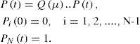
It is complex to solve this problem with continuous lead time with use of analytical methods. Therefore, we try to use approximate method. For this purpose, the continuous time system turns out to be discrete and the optimal control problem is converted into equivalent nonlinear programming. On the other hand, differential relations in set of relations 12 are converted to difference equations. Integral expressions are converted to summation ones. For progress of this method, time has been divided into K equal sections with length of Δt.
If Δt is small, we can assume that P(t) changes only at times 0,Δt,...,(K-1)Δt. Therefore, if P(kΔt) is shown with kthp with P(k), the continuous time system P(t) = Q(μ)..P (t) is converted to discrete time system.

Mixed integer nonlinear programming model is obtained which is equivalent to the main model with which μ=μ1*,μ2*,...,μn*T or the optimal control vector is obtained.
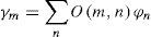
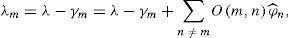
With regard to hypothesis governing the problem, input rate or system input distribution parameter is λ and since lack of wastes has been assumed in all stations, therefore, it is evident that the input rate of all stations will be λ. Now, if you assume that each station has irreversible wastes which have been shown with γm, each servicing station input rate will not be equal to λ. Therefore, we can showmth servicing station input rate with λm and we can write as follows:

Where γm is defined as wastes of the previous servicing stations and m servicing stations. Now if the relationship between stations is shown on the basis of production process with matrix O(m, n) we can calculate value of γm for servicing stations:
Where ϕn indicates wastes of mth station which is independent of wastes of other stations. It is necessary to note that the parts of which equivalent part or parts are regarded as wastes in assembly station are regarded as a kind of wastes:
If q(i,j,m) is three-dimensional matrix with entries -1,0,+1 and defined as follows:
If ≠ j, the entry relating to servicing stations of which activities have been finished takes value of 1 during change from state i to j.
If qi,j,m=−∑k≠iqi,j,m, ∀m. :i=j then we can define matrix Qγ, as follows:

In order to insert wastes in model (14), matrix Q’ is defined as follows:

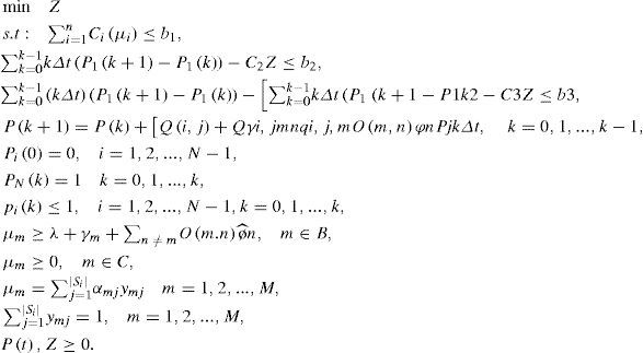
Relation (13) will change as follows:

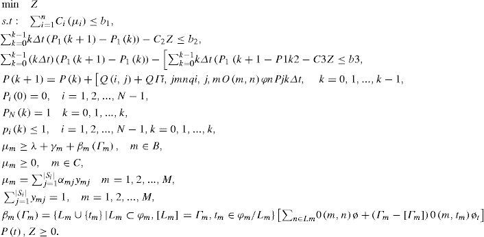
In which, model (20) will emerge by subtitling relation 19 with its equivalent constraints in the model (14) and expanding constraint relating to stability with use of relation (15):
The introduced model is valid in set of relations (20) when its parameters are defined finally. In case waste in each station is indefinite in each station ϕn, the validity of the following model will be questioned. In order to confront with this uncertainty, robust optimization is used.
5Robust multi-objective lead time control problemIn order to achieve a robust answer for multi-objective lead time control problem (MOLTCP), robust multi-objective lead time control problem (RMOLTCP) are presented with the use of two robust optimization approaches.
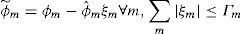
5.1Robust model for interval uncertaintyAssume that wastes in independent stochastic variables servicing stations ϕ˜;m which have symmetric distribution in theinterval φm−φˆm,φm+φˆm⋅ψm is a set of machines relating to machine m where ϕ˜; is indefinite.
Therefore, we can show wastes in each station as follows:

Where, ξm is stochastic variable between -1 and +1 which shows data fluctuations. In this case, all elements of ξ vector can change in interval [-1,1] which is called an interval uncertainty model. This robust optimization method in linear programming was presented for the first time by Soyster (1973). Since this method optimizes the worst state, it is regarded as conservative method. In this method, it is assumed that the worst state occurs for all indefinite parameters On the other hand, it takes the minimum value in the studied problem of ϕ˜;m. In this regard, input rate of each station increases, which changes the stability of queue system and average values and variance by changing P(k). Since we want to optimize the worst state, therefore, the value of λm is defined as follows:
The MOLTCP problem solution is modeled with use of relations (20) and (22).
This method, which is the most conservative robust optimization method is very simple and metaheuristic methods can be used for solving MOLTCP problema. But since you have assumed the worst state, it decease value of the target function. A robust optimization method of which conservative rate is adjusted is explained for MOLTCP problem. (Dalfard, 2014), (Kaveh et.al, 2014).
5.2Robust optimization with use of budget uncertainty modelMany efforts have been done to remove defect of Soyster’s method which acts conservatively. Ben-Tal and Nemirovski (1998,1999, 2000), El-Ghaoui and Lebret (1997) and El-Ghaouiet.al (1998) presented methods for solving this case. But his suggested methods have some disadvantages which make the robustness problem and inapplicability of optimization problems difficult with discrete variables.
For discrete problems, Kouvelis, and Yu (1997) presented a robust discrete optimization framework which seeks to find the answer for minimizing performance of the worst state under a series of scenarios for the parameters.
Unfortunately, robust peers of many discrete optimization problems which can be solved in polynomial time are converted to NP-Hard problems. Bertsimas and Sym (2002, 2004) presented a robust optimization method for linear programming problems of which conservative rate can be adjusted and doesn’t increase the difficulty of the problem. One of the advantages of this method is its applicability to discrete optimization of problems and mixed optimization ones. A method, in which this uncertainty is budgetary, is assuming that the maximum number of Гmvaries between rates of m machine wastes. Parameter Г is called protection level and is a nonnegative integer smaller than or equal to the number of indefinite parameters relating to the wastes. When it changes by maximum number of Г, robust optimal answers will be obtained and will remain optimal. Method, in which this is an approximation of the robust optimization with interval uncertainty, it is assumed that:
We will have the following model by applying this method on MOLTCP problem.
We can show that the introduced model in set of relations (25) is equivalent to the following model:
With regard to constraints and variables to be added, the number of the added variables and constrains in model (26) will be equal L,m + L in comparison to the model (20) which is
5.2.1Proof
For βm (Гm), Гm equals to the optimal answer obtained from the following model.
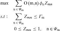
Combination of model (7) is as follows:
Since, βm(Гm) is equal to optimal answer (27) and it equals to answer (28), therefore, equivalence of model (25) and (26) is obtained.
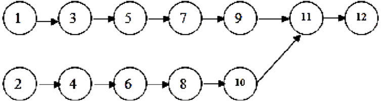
6Experimental results:For a numerical study of the problem, assume a dynamic assembly system in figure 1 in which speed of demand for each product unit equals to 15 per day and assume that all service stations follow queue system M/M/1.

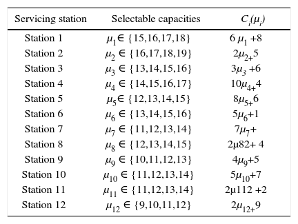
Characteristics of servicing stations include function relating to calculation of each unit cost in Rials and set of selectable capacities for each servicing station are given in table 1.
Characteristics of servicing stations.
| Servicing station | Selectable capacities | Ci(μi) |
|---|---|---|
| Station 1 | μ1∈ {15,16,17,18} | 6 μ1 +8 |
| Station 2 | μ2 ∈ {16,17,18,19} | 2μ2+5 |
| Station 3 | μ3 ∈ {13,14,15,16} | 3μ3 +6 |
| Station 4 | μ4 ∈ {14,15,16,17} | 10μ4+4 |
| Station 5 | μ5∈ {12,13,14,15} | 8μ5+6 |
| Station 6 | μ6 ∈ {13,14,15,16} | 5μ6+1 |
| Station 7 | μ7 ∈ {11,12,13,14} | 7μ7+ |
| Station 8 | μ8 ∈ {12,13,14,15} | 2μ82+ 4 |
| Station 9 | μ9 ∈ {10,11,12,13} | 4μ9+5 |
| Station 10 | μ10 ∈ {11,12,13,14} | 5μ10+7 |
| Station 11 | μ11 ∈ {11,12,13,14} | 2μ112 +2 |
| Station 12 | μ12 ∈ {9,10,11,12} | 2μ12+9 |
Stochastic process of {X(t)t ≥ 0} which relates to analysis of the longest route of the stochastic network has 38 expressions which are as follows:

The ideal goal for operational costs of the system per day is b1=890 Rls,b2=2.3 days, and b3=0.03 squared days for average and variance of lead time. With regard to the fact that a day of deviation from average lead time is 100 times more important than one Rial difference in total operational expenses of the system and is as important as one squared day of difference from the lead time variance. Then values cj will be c1 =0.9804 and c2=c3=0.0098. Other values of parameters will be Δt= 0.334,k= 25 and ε= 0.05.
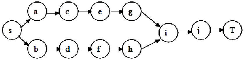
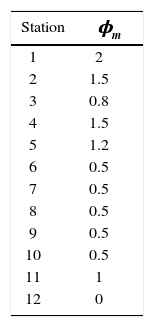
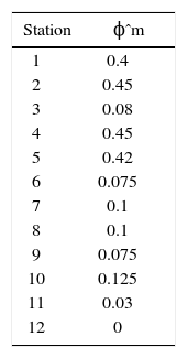
Table 2 shows wastes of servicing stations. Figure 2 shows queue network equivalent stochastic network presented in figure 1 of which edges are independent of each other and have been distributed exponentially.

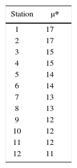
Table 3 shows optimal servicing speeds or μ* for i= 1,2,…,12
Table 4 shows lead time distribution function in the production system at kΔt and k= 1,2,...,25
Now, it is assumed that changes of wastes in each station ϕˆm equals to the rate given in table 5.
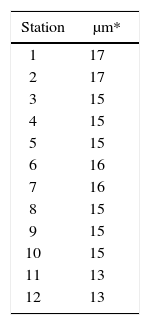
With regard to the specified values for parameters, results obtained from robust optimization for total cost of system in one day, average lead time, lead time variance are as follows and average servicing rate in stations (optimal speeds) is based on table 7.

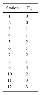
With regard to Bertsimas and Sym (2004) and with regard to what is given in table 5, value of Гm is based on table 6.
At the end, minimum operational cost of the production system per day, average minimum and minimum lead time variance are obtained as follows:

As observed definite answer, average servicing rate is higher than the results obtained from definite model and production cost and average lead time increase and their variance decreases.
ConclusionIn this article, a new multi-objective model has been suggested with regard to irreversible wastes in an indefinite state for optimal control of servicing speeds of production and assembly operations in a multiphase assembly system. The average lead time and variance and total operational costs of the system are minimized in each period. In this model, wastes are regarded as defining element in the system. Then two robust optimization methods are used for including uncertainty in the related parameters. It is difficult to solve problem in continuous state. Therefore, the problem is solved through estimation and by making continuous time system discrete and converting optimal control problem to an equivalent nonlinear programming. The limitation of this model is that the number of variables and constraints of multi-objective nonlinear programming increases exponentially with increase of network size. Methodology can be expanded in the following fields:
Using Mont Carlo simulation for analyzing the effect of non-exponential inputs on times of operation, transportation and their related wastes.
One interactional method such as the surrogate worth trade off method, STEM or SEMOPS can be applied for solving robust multi-objective lead time control problem.