

The standard analysis of the impact of EPL on labour market outcomes concentrates mainly on unemployment and job flows, disregarding possible effects on labour productivity. In this paper we make (a component of) labour productivity endogenous and analyze how the presence of a stringent protection legislation affects labour market in an equilibrium matching model with endogenous job destruction. In particular, in our study we imagine that an employed worker has to exert effort to produce and this generates disutility. Therefore, in this framework high labour productivity on one hand is costly for a worker in terms of disutility, and on the other hand might be beneficial in terms of lower job destruction. We find that high firing costs partially substitute high labour productivity in reducing job destruction and this, consequently, brings down the optimal level of productivity. Furthermore, the impact of EPL on unemployment is ambiguous but numerical exercises show unambiguously how higher firing restrictions reduce different measures of aggregate welfare. To some extent, the clear emergence of these results leads to interesting policy implications and, indeed, rationalizes the recent empirical evidence on the impact of EPL.
El análisis estándar del impacto de la EPL sobre los resultados en el mercado laboral se concentra sobre todo en el paro y en los flujos de trabajo y paro. En este documento hacemos endógena (un componente de) la productividad laboral y analizamos cómo afecta al mercado laboral la presencia de una legislación de protección rigurosa en un modelo combinado de equilibrio apropiado con la destrucción de empleo endógena. Concretamente, en nuestro estudio imaginamos que un trabajador por cuenta ajena debe hacer esfuerzos para producir y esto genera desutilidad. Por lo tanto, dentro de este marco, para un trabajador la alta productividad laboral es costosa en términos de desutilidad, pero también puede ser beneficiosa por lo que se refiere a la menor destrucción de empleo. Observamos que el alto coste del despido sustituye parcialmente la alta productividad laboral al reducir la destrucción de empleo y, en consecuencia, esto reduce el nivel óptimo de productividad. Además, el impacto de la EPL sobre el desempleo es ambiguo, pero los cálculos numéricos muestran de manera evidente cómo las mayores restricciones del despido reducen diferentes medidas de bienestar global. En cierta medida, la aparición evidente de estos resultados conlleva implicaciones normativas interesantes y, lo que es más, racionaliza la evidencia empírica reciente sobre el impacto de la EPL.
Recent empirical evidence from European countries and the US shows that the presence of stringent employment protection legislation (EPL) affects significantly labour productivity. In particular, cross-country (DeFreitas and Marshall, 1998), diff-in-diff (Micco and Pages, 2006; Autor et al., 2006, 2007; Bassanini and Venn, 2007; Bassanini et al., 2009; Lisi, 2013) and other studies (Riphahn, 2004; Ichino and Riphahn, 2005) found that higher EPL have a negative impact on labour productivity.
Nonetheless, standard theoretical analysis of EPL focuses mainly on unemployment and job flows, disregarding possible effects on labour productivity. In particular, both standard analysis of labour demand under uncertainty (Bentolila and Bertola, 1990; Bertola, 1990; Bentolila and Saint-Paul, 1992; Bentolila and Dolado, 1994; Boeri and Garibaldi, 2007) and general equilibrium models (Mortensen and Pissarides, 1994, 1999b; Garibaldi, 1998; Pissarides, 2000; Cahuc and Postel-Vinay, 2002) tend to consider an exogenous productivity, not influenced by the presence of labour-market policies. Indeed, some studies analyze the role of EPL in distorting the adjustment of employment and investment, consequently affecting productivity (Hopenhayn and Rogerson, 1993; Saint-Paul, 1997, 2002; Bartelsman and Hinloopen, 2005).
In this paper, in the spirit of Ichino and Riphahn (2005), we concentrate more on the behavioural component of productivity. Therefore, we make (a component of) labour productivity an endogenous object of the model and, then, study the impact of a stringent protection legislation. Since our concern is to understand the equilibrium impact on productivity, unemployment and welfare, we need to embed the analysis into an equilibrium model of the labour market. To this extent, the matching approach to equilibrium unemployment should represent the best candidate for this kind of analysis.
In the canonical matching model total productivity is usually characterized by an exogenous common component, affecting productivity in all jobs, and an idiosyncratic component, governed by a stochastic process. Indeed, in such specification of productivity there do not seem to be place for workers. Differently, in our study we imagine that an employed worker has to exert effort to produce and this generates disutility. Following this argument, we assume that a component of productivity is determined by the level of effort exerted by workers. Thus, in this framework high labour productivity on one hand is costly for a worker in terms of disutility, and on the other hand might be beneficial in terms of lower job destruction. Since stringent protection legislation has the same well-known effect of reducing job destruction (e.g. Pissarides, 2000), EPL might affect total productivity also through this behavioural component. Therefore, the novelty introduced in this paper should contribute to offer a more comprehensive evaluation of the impact of EPL on labour productivity and, more generally, on labour-market outcomes.
An equilibrium is a job destruction and job creation rule, a labour productivity and a level of unemployment implied by the rational expectations behaviour of individual firms and workers and by the matching technology. We study how the presence of a stringent protection legislation affects productivity, unemployment and welfare in the aggregate steady-state. We find that high firing costs partially substitute high labour productivity in reducing job destruction and this, consequently, brings down the equilibrium labour productivity. Furthermore, the impact of EPL on unemployment is ambiguous but numerical exercises show unambiguously how higher firing restrictions reduce different measures of aggregate welfare. To some extent, the clear emergence of these results leads to interesting policy implications, especially in the light of the great debate emerged in the last years regarding EPL. Moreover, the extension pursued in this paper would offer a reasonable interpretation to rationalize the recent evidence on the negative impact of EPL on productivity. Indeed, this approach to consider labour market outcomes and personnel economics together in addressing policy questions has already turned out to be successful (see e.g. Shapiro and Stiglitz, 1984).
In regards to how this paper places in that strand of literature aiming to evaluate the impact of EPL, the main contribution consists in introducing labour productivity (besides unemployment and job flows) in the general equilibrium evaluation of this particular policy in the labour market. To this extent, the paper shares the same spirit of Lagos (2006). In particular, that paper proposes an aggregative model of TFP in the matching framework, allowing to evaluate the impact of labour-market policies on the general aggregate production function and, especially, on average TFP. Nonetheless, in Lagos (2006) higher firing costs affect TFP only by reducing firms’ job destruction in response to negative shocks, implying a lower average idiosyncratic productivity of active units. Indeed, in the model proposed here we will see that a more comprehensive evaluation of EPL, beyond the impact on the average idiosyncratic component, should consider also the impact on the behavioural component of productivity.
On the other hand, this paper is also close to Dolado et al. (2011), aiming to evaluate the impact of having large differences between EPL for permanent and temporary contracts on endogenous workers’ effort and firms’ conversion rates. Interestingly, they find that an increase in firing costs gap would lead to a reduction in both firms’ conversion rate and effort exerted by temporary workers. Nonetheless, as stated in their paper, they focus on temporary contracts insomuch as they still consider productivity for permanent employment exogenous and, in turn, not influenced by protection legislation. Moreover, in order to stress the mechanism linking firing costs to conversion rates and temporary workers, they work in a partial equilibrium framework under different assumptions.1 Differently, in this paper we aim to underline the key mechanism whereby EPL could affect average labour productivity of regular workers in a general equilibrium framework, that is, not only by reducing average idiosyncratic productivity of active units, but also by substituting high labour productivity in containing job destruction.
The rest of the paper proceeds as follows: in Section 2 we describe the basic theoretical framework and in Section 3 characterize its steady-state. Section 4 studies qualitatively the impact of a stringent protection legislation on the equilibrium level. In Section 5 we conduct some numerical exercise to study the effect on productivity, but also on different measure of aggregate welfare. Section 6 concludes. Finally, Appendix A contains some useful derivations.
2The theoretical frameworkThe basic theoretical framework is the matching approach to equilibrium unemployment with endogenous job destruction (e.g. Pissarides, 2000). In this economy there is an endogenously sized continuum of jobs, characterized by a common component of productivity p and an idiosyncratic component x. Each product commands in the market a price of px, which evidently differs from each other for the presence of the idiosyncratic component. In standard versions of this model p is usually considered an exogenous parameter, capturing macro events that affect productivity in all jobs by the same amount and in the same direction. Differently, in this paper we interpret p as the behavioural component of labour productivity, with x still representing the idiosyncratic condition in the market, due to demand or technology. Therefore, in our model we do not consider p a parameter capturing macro shocks, because our aim is indeed to study how firing costs affect the level of the behavioural component of productivity. However, it is evident that there is no difficulty in including also such parameter in our model.
The stochastic process governing the idiosyncratic component x is Poisson with arrival rate λ. Whenever a jump arrives, the new level of x is drawn from the distribution G(x) with finite upper support x¯ and no mass point. The Poisson process implies that shocks are persistent, but conditional on change the new draws are independent by the initial level of x.
Each firm has only one job that can be either filled and producing some good (state J(x)), according to the idiosyncratic level x and the behavioural productivity p, or vacant and searching for a worker (state V), which costs pc per unit of time. Firms have full information on technology and market condition, therefore they create always the most profitable job, that is, with the idiosyncratic level at the upper support of the price distribution. Furthermore, the Nash bargaining rule implies also that new jobs offer the highest wage. However, investments are irreversible and when a shock arrives firms have no choice over their productivity. Filled jobs not always resist to negative productivity shocks and, in particular, they are destroyed whenever the new draw of x falls below a certain level of reservation productivity R. This implies that each job has a probability of being destroyed equal to λG(R). Job destruction is not costless, rather whenever a job is destroyed firm has to pay the firing costs pF.
Respectively, each worker can be in one of two states, employed and producing some good (state W(x)) or unemployed and searching for a job (state U). Employed worker receives the wage w(x) and has to choose how much effort e to exert in the job, which determines the common component of productivity p=f(e). Even if not necessary, we assume a linear relation p=e between effort and productivity.2 On the contrary, unemployed worker does not exert effort and benefits only from z, which can be interpreted either as unemployment compensation or as leisure. Wages are the outcome of the Nash bargaining, according to which workers receive a fraction 0<β<1 of the match surplus, where β can be interpreted as the workers’ bargaining power. Since the match surplus is conditional on idiosyncratic productivity, wages are revised whenever a productivity shock occurs. In particular, it is intuitive that both match surplus and wage are increasing function of x. Following the previous literature, we assume that workers are risk neutral and impatient, which implies zero saving and full consumption. Furthermore, exerting effort generates an increasing disutility. Therefore, an employed worker enjoys conditional on x the instantaneous utility
where γ is the parameter governing marginal disutility of effort (see e.g. Garibaldi, 2006), whereas the instantaneous utility of the unemployed worker is simply

The number of matches between vacant jobs and unemployed workers is governed by a canonical matching function m(v, u), where v and u are respectively the number of vacant jobs and unemployed workers. Labour force is normalized to 1, so that in this economy the number of unemployed workers u is the unemployment rate. As standard in the literature, we assume that the matching function is twice continuously differentiable, increasing and concave in both its arguments and homogeneous of degree one, with elasticity strictly between 0<ξ<1. By linear homogeneity, the transition rate from vacant to filled job is m(v, u)/v=m(1, u/v)=q(θ), with q′(θ)<0, where θ=v/u identifies the labour market tightness. Moreover, the elasticity of q(θ) is strictly between −1<η<0 and it is related with the elasticity of the matching function (respect to v) by η=ξ−1. Similarly, the transition probability from unemployed to employed is m(v, u)/u=m(v/u, 1)=θq(θ), an increasing function of θ.
Thus, the endogenous variables of the model are the level of market tightness θ, the level of reservation productivity R, the level of effort e and, in turn, labour productivity p and the level of unemployment u. In the next section we characterize and derive their steady-state values.
3Steady-state equilibriumIn steady-state the choice of opening a vacancy and destroying a job for a firm, as well as the level of effort for a worker, are based on their asset values. Indeed, these values are fairly similar to those in a canonical matching model (e.g. Pissarides, 2000), with the difference of the effort level in the worker utility function. Therefore, the inclusion of effort does not change heavily the asset values, but it does change significantly the subsequent steady-state analysis.
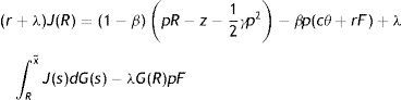
From the assumptions on vacancy cost, idiosyncratic component and firing costs, we have that the asset values of a vacancy and a filled job satisfy the following Bellman equations:


In (1) a firm has to pay the vacancy cost per unit of time – pc and with probability q(θ) matches with an unemployed worker, gives up the value of a vacancy V and gets the value of a filled job at the upper support of the price distribution J(x¯). In steady-state vacancies are opened until all rents are exhausted. Therefore, the equilibrium zero-profit condition is
In (2), conditional on the idiosyncratic productivity, a firm enjoys the value of product px and pay the wage w(x), then with probability λ a shock arrives and a new level of x is drawn from the price distribution G(x). In this case the firm has to give up the value J(x) and gets the new value J(s) if s is over the reservation productivity R, or destroys the job and pay firing costs pF in case the new draw s is under R.
Similarly, from the assumptions on unemployment compensation (or leisure) and instantaneous utility function, the asset values of unemployed and employed worker satisfy
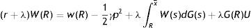
In (4) an unemployed worker enjoys the unemployment compensation z and with probability θq(θ) matches with a vacant job, gives up the value U and gets the value of being employed at the upper support of the price distribution W(x¯). In (5), conditional on the idiosyncratic productivity, an employed worker enjoys the wage w(x) but suffers the effort exerted −(1/2)γe2, then with probability λ a shock arrives and a new level of x is drawn from the price distribution G(x). In this case the worker has to give up the value W(x) and gets the new value W(s) if s is over the reservation productivity R, or the value of unemployed U in case the new draw s is under R. Furthermore, as will be more clear below, e is the effort level maximizing the asset value of being employed, since we characterize the equilibrium under rational expectations.
Nash bargaining implies that workers receive a fraction β of the total match surplus, which is revised whenever a productivity shock occurs. However, the total match surplus of a new job is different from that of an existing job, because only in an existing job firms save firing costs for the continuation of the match. Therefore, as standard in the matching literature, we have to distinguish between the outside w0 and the inside wage w(x).
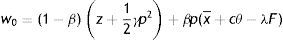
In the case of a new job the match surplus is
and the sharing rule implies

Using the relation p=e, the zero-profit condition (3), the asset equations for a filled job (2), unemployed (4) and employed worker (5) and the sharing rule (6), gives the outside wage equation3
Differently, in the case of an existing job a firm saves firing costs for the continuation of the match and, consequently, the match surplus changes in the following

and the sharing rule implies

Following the same argument, we get the inside wage equation
Eqs. (7) and (8) differ only for the impact of firing costs F and, indeed, this difference emphasizes the standard conflict between insiders and outsiders. On one hand, inside a match the prospect of paying F leads firms to concede marginally a higher wage to avoid the destruction of existing jobs. On the other hand, outside a match the expectation of paying firing costs, when the job will be destroyed, leads firms to start the new match with a lower wage to partially recoup the future payment of F. Moreover, as (7) clearly shows the impact of F on the outside wage is higher when λ is higher, because the probability of job destruction is greater.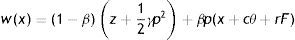
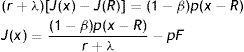
The choice of destroying a job is taken inside a match, therefore we use the inside wage equation to derive the job destruction condition. Substituting (8) in (2), we get a more explicit expression of the asset value of a filled job J(x) as a function of the idiosyncratic component
From (9) we can see that J(x) is a monotonically increasing function of x. This implies that there exists a unique value x* such that J(x*)=0 and, in turn, for any x greater (smaller) than x*, then J(x)>0 (J(x)<0). In the model without firing costs, this implies that the reservation productivity R, under which a firm destroys a job, satisfies the reservation property J(R)=0. Differently, with firing costs for a firm is optimal to continue even a negative match, as far as the negative surplus is smaller than the cost of destroying a job pF. Therefore, with firing costs the reservation property is J(R)=−pF (or W(R)=U), which allows us to characterize the reservation productivity R.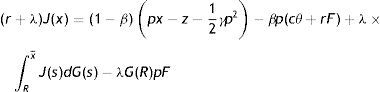
Evaluating the generic asset equation of a filled job J(x) at x=R, we have the following
Now, subtracting equation J(R) from the generic asset equation (9) and, then, using the reservation property J(R)=−pF, we get
Finally, substituting (11) in the integral expression of (10) and dividing by (1−β)p, we get an implicit expression for R as a function of market tightness θ, labour productivity p and the parameters of the model
Eq. (12) is the first steady-state condition of the model. In what follow we will refer to this as the job destruction rule (JD), when we emphasize the relation between R and θ, or as the reservation equation (RE), when we emphasize the relation between R and p.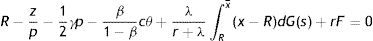
The value of pR is the lowest acceptable price to continue a job. Moreover, from (12) we can see that pR is lower than the reservation wage (rU=z+(β/1−β)pcθ), which is the lowest acceptable wage for a worker. One reason is the presence of firing costs, which are paid by firms but not enjoyed by workers. The other reason standard in this literature is the presence of labour hoarding, represented by the integral expression. In particular, given the probability that the idiosyncratic productivity x might change in the future, for a firm is optimal to continue some negative match and wait for a higher price, in order to avoid the hiring cost. As intuitive, labour hoarding is increasing in the probability of a change λ.
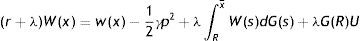
On the other hand, the choice of creating a job is taken outside the match; therefore we use the outside wage equation and evaluate the value of a filled job at the upper support of the price distribution. Substituting (7) in (2), subtracting (10) and using J(R)=−pF, we get
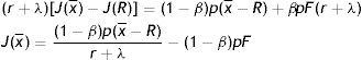
Finally, inserting the zero-profit condition (3) in (13), we get an implicit expression for θ as a function of the reservation productivity R and the parameters of the model
Eq. (14) is the second equilibrium condition and we will refer to this as the job creation condition (JC). The left hand side of (14) is the cost of a vacancy for the expected duration of filling a vacancy. The right hand side is the discounted additional surplus a firm gets from a new job. Therefore, this condition says that in equilibrium the expected hiring cost of a new vacancy has to be equal to the expected gain from a new job.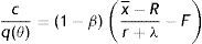
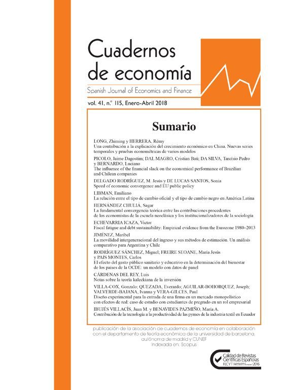
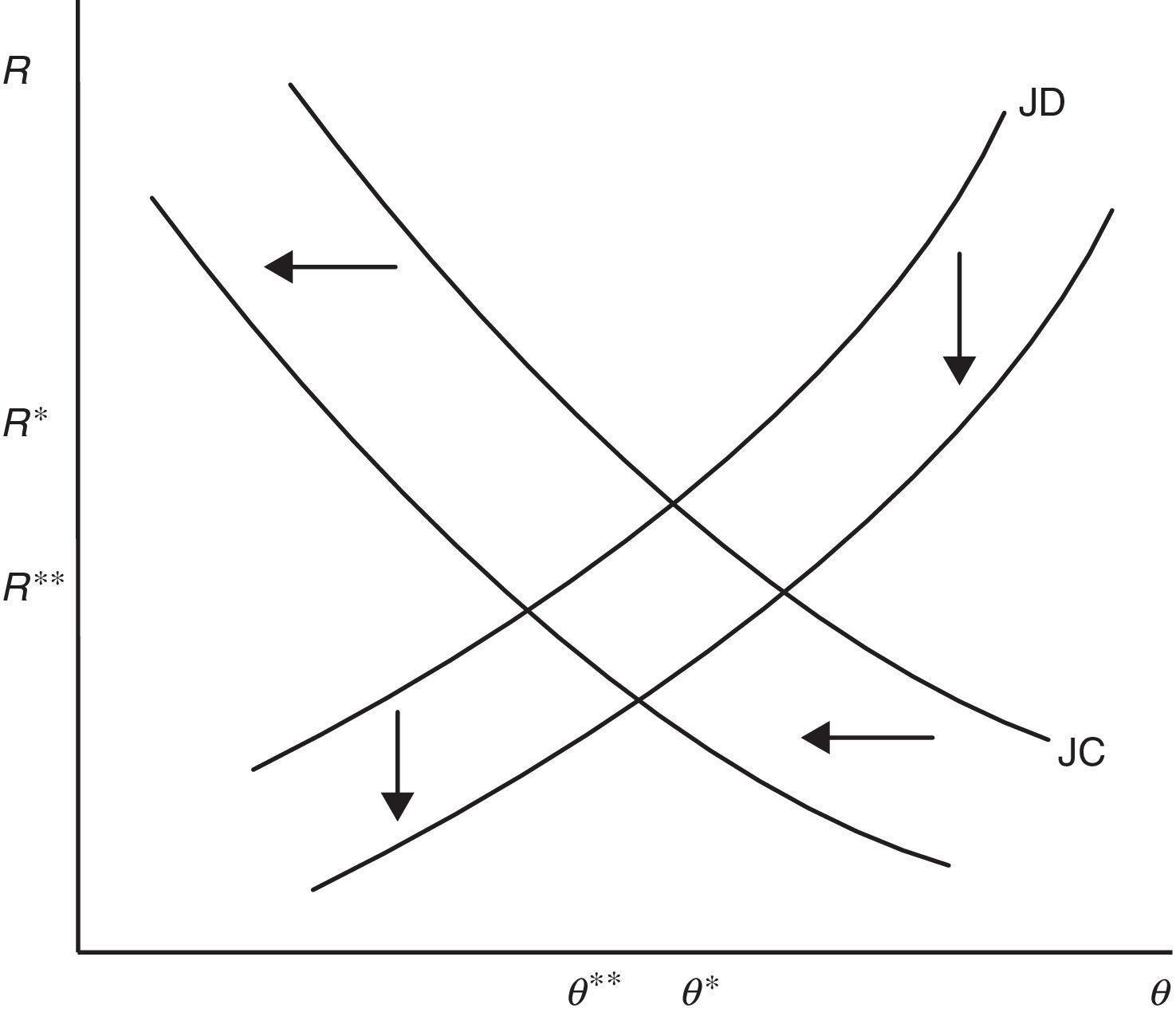
Eqs. (12) and (14) jointly determine R and θ, as illustrated in Fig. 1. Let us define (12) as B(R,θ,p,ω)=0 and (14) as D(θ,R,ω)=0, where ω is the set of parameters. Then, we have
As (15) shows, the curve JD slopes up because a higher θ increases the probability of finding a job and, thus, the opportunity cost for a worker ((β/(1−β))cθ), who now pretends a higher wage to accept a job and, consequently, more jobs are marginally destroyed. On the other hand, from (16) we know that the curve JC slopes down because a higher R increases the probability that a job is destroyed λG(R) and, in turn, reduces the expected gain from a new job ((1−β)((x¯–R)/(r+λ))), so less vacancies are opened.


So far, the joint determination of R and θ (for a given level of labour productivity p) has followed the previous literature and, indeed, besides the different specification of the worker utility function, no significant novelty have been introduced. However, in our model labour productivity is not a parameter, but an ulterior endogenous to be studied. Following our interpretation of p as behavioural component of productivity, we assumed that it is determined by the level of effort e exerted by the employed worker and, in particular, that p=e.
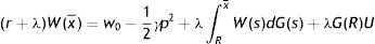
The choice of effort is rationally taken by workers when they match with a vacant job, therefore in equilibrium e maximizes the value of being employed at the upper support of the price distribution W(x¯). In particular, when a worker takes this choice he actually knows the job destruction rule R and, thus, takes into account the impact on it. Moreover, given the choice of effort is taken individually, the single worker considers the impact on market tightness θ marginally negligible. From this, it can be easily seen that the same effort level maximizes the asset value of unemployment, being U a monotonically increasing function of W(x¯)

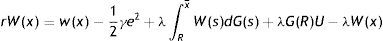
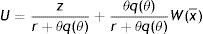
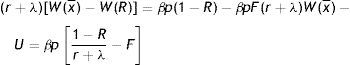
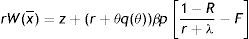
The maximization of W(x¯) in the form of Bellman equation (5) is not a trivial calculus. However, using p=e and the reservation property W(R)=U, Eqs. (4) and (5) can be solved for the permanent income form as a function of R, θ, p and the parameters of the model (see Appendix A)
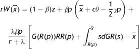
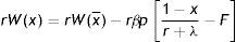
Intuitively, since there is a non-zero probability of a productivity shock and, all the more so, of being fired, the permanent income of an employed worker at the upper support of the price distribution is less than his instantaneous utility. The permanent income form (17) allows us to take the F.O.C. and characterize the equilibrium condition for labour productivity p∂rW(x¯)/∂p=0
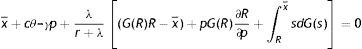
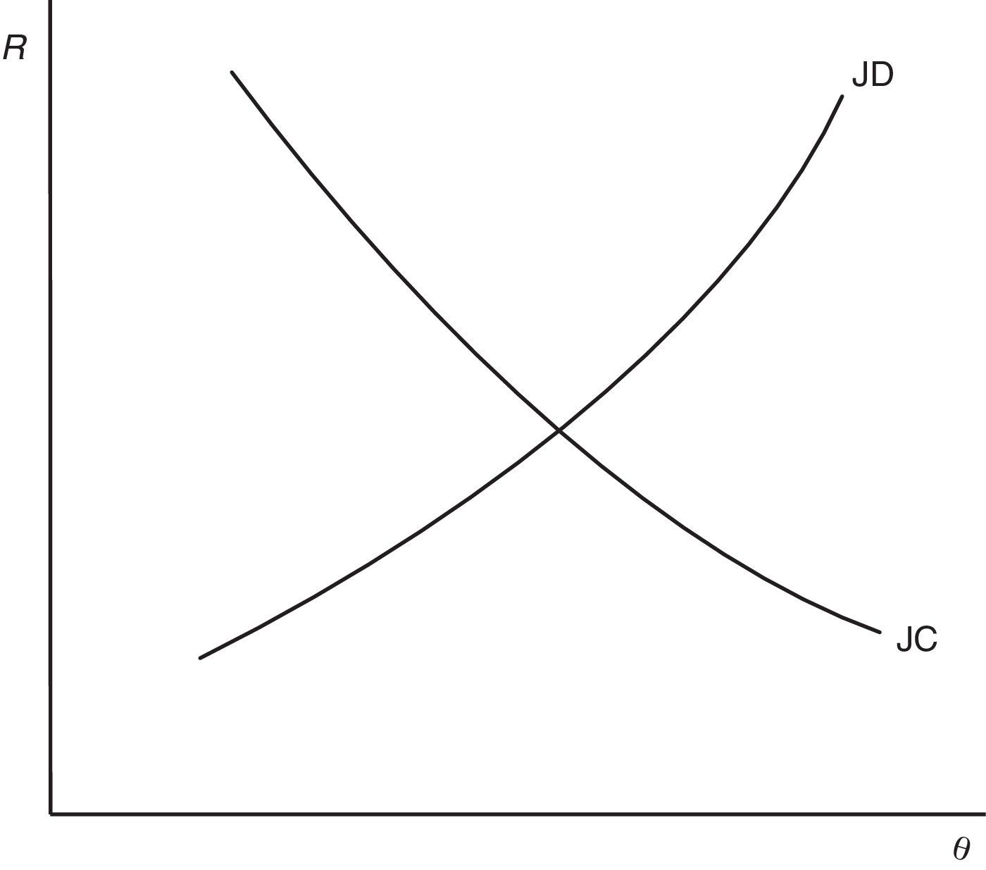
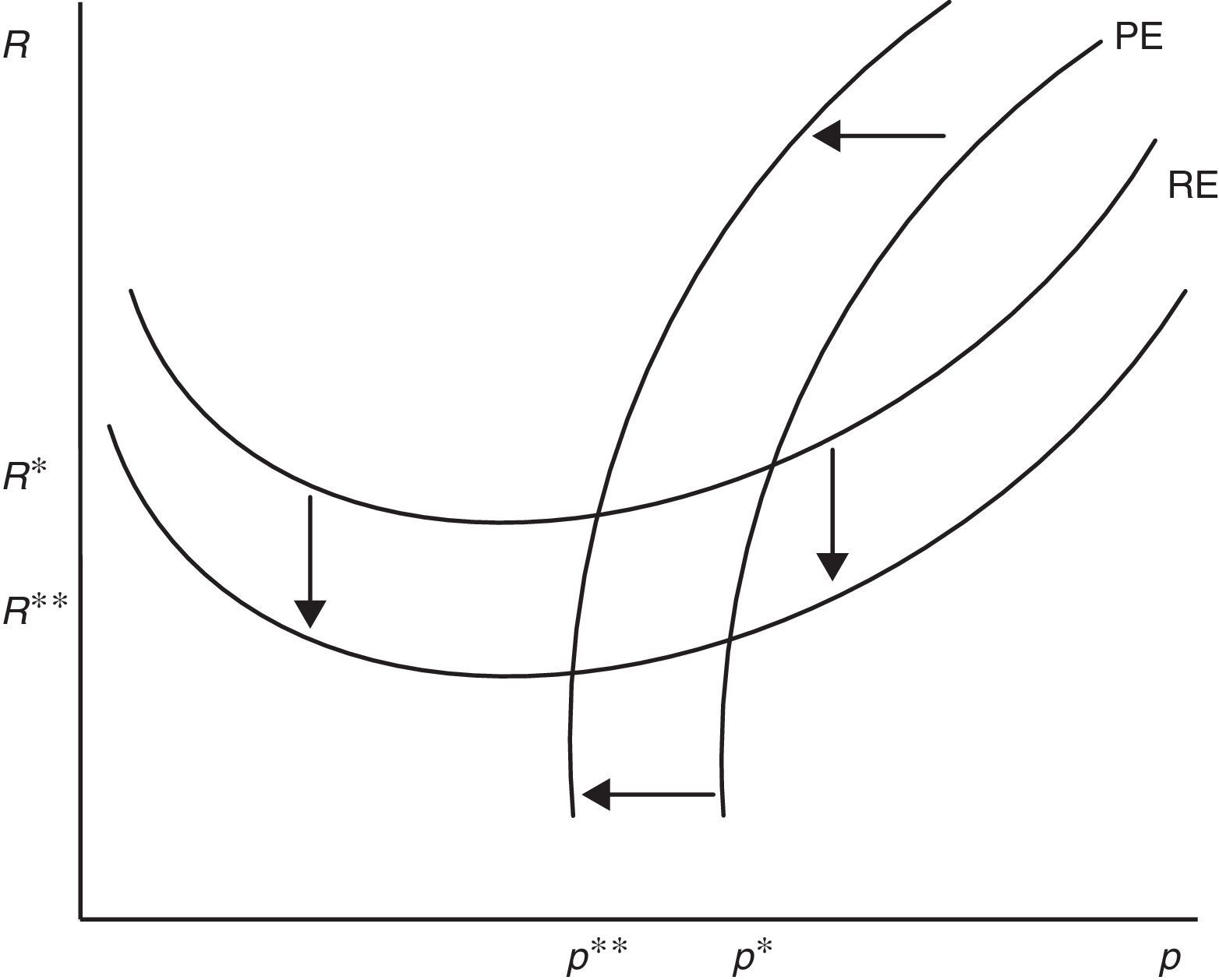
Eq. (18) represents the equilibrium condition for labour productivity p (or effort e)4 and from now on will be called the productivity equation (PE). From (18), we can notice that the optimal level of p depends on R and θ. Differently, from (12) and (14) we can see that only RE depends on p. Therefore, for any level of market tightness θ, PE and RE jointly determine R and p, as illustrated in Fig. 2. The shape of these curves is a bit more complicated than JC and JD, but still intuitive. Remembering that we defined the PE (12) as B(R,θ,p,ω)=0 and, now, defining Eq. (18) as M(p,R,θ,ω)=0, we have the following
Looking at (19), labour productivity p has two opposite effects on optimal reservation productivity R, the disutility-wage effect and the production effect. On one hand, a higher p increases the disutility of worker and consequently the wage (−(1/2)γp), thus more jobs are marginally destroyed. On the other hand, a higher p increases the value of production (pR) and partially compensates a lower x, leading to a fall in R. Nonetheless, because of the increasing marginal disutility of effort, we can establish that when p is low the effect on wage is relatively small and the effect on production dominates; on the other hand, when p is high the disutility increases more than proportionally and the effect on wage dominates. Therefore, RE has a standard u-shape, with a minimum in the point in which disutility-wage effect and production effect exactly compensate.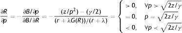


Similarly, reservation productivity R affects labour productivity p for the continuation value effect. In fact, a marginal increase in R does not change the instantaneous utility of worker, but certainly it does change his continuation value. In particular, a higher R not only increases the probability of being fired (λG(R)), shortening the expected period of employment, but also decreases the probability of finding a job (θq(θ)), increasing the expected period of unemployment. Indeed, both these impacts affect negatively the continuation value and, therefore, the worker chooses p also in order to address optimally the level of R through (12). This continuation value effect is included in the numerator of (20) and it is greater for R and p high, implying the PE shape showed in Fig. 2.
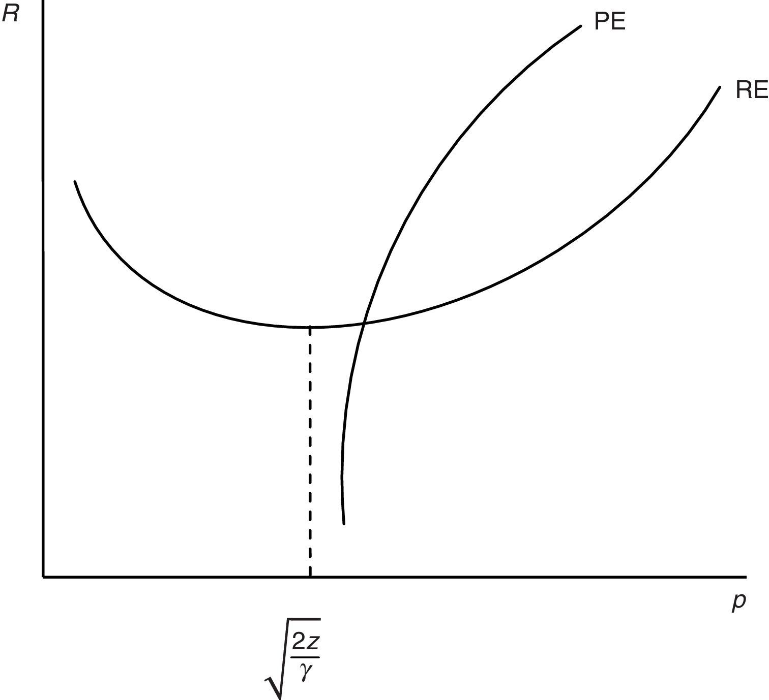
The last equation of the model is the steady-state condition for unemployment, the so-called Beveridge Curve. Indeed, there are different ways to derive this condition, here we state it in terms of flows in and flows out unemployment. In equilibrium the number of workers who enter unemployment (1−u)λG(R) has to be equal to the number of workers who leave unemployment uθq(θ). Therefore, the steady-state condition for unemployment is
Eq. (21) is the final equilibrium condition of the model and implies that in equilibrium, for any values of R and θ, there is a unique unemployment rate u and, in turn, a unique number of vacant jobs v.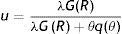
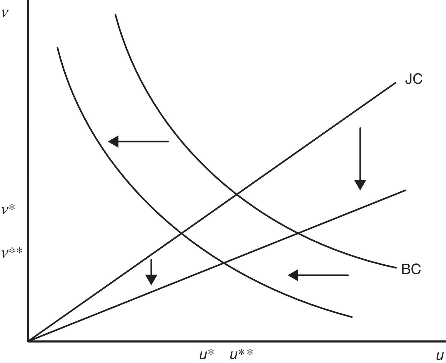
The Beveridge Curve is often drawn in vacancy-unemployment space by a downward sloping and convex curve. Indeed, as highlighted by Mortensen and Pissarides (1994), in the matching model with endogenous job destruction the precise shape of the Beveridge Curve is ambiguous. In particular, differentiation of (21) shows that there are two opposite effects
On one hand, more vacancies increase the number of job matches, implying a lower unemployment rate, captured by the second term of the denominator (22). On the other hand, more vacancies increase the number of jobs destroyed, implying a higher unemployment rate, the first term of the denominator (22). Despite this ambiguity, since the empirical evidence seems to support the conventional shape, it is common to assume that the matching effect is stronger than the destruction one and, thus, to draw the Beveridge Curve as a downward sloping and convex curve. In this regard, the numerical simulation of our model with the equilibrium values also confirms this conventional form. Therefore, in Fig. 3 we draw Eq. (21) as a downward sloping and convex curve. As usual, we draw the Beveridge Curve with a straight line through the origin, representing all the possible values for v and u compatible with the equilibrium market tightness θ.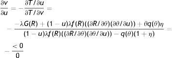

In conclusion, we are ready to define the rational expectations equilibrium of the model: Steady-state equilibrium – The rational expectations equilibrium is a quadruple (R*, θ*, p*, u*) that satisfies the job destruction condition (12), the job creation condition (14), the productivity equation (18) and the Beveridge Curve (21) implied by the rational expectations behaviour of individual firms and workers and by the matching technology.
For any value of labour productivity p, Eqs. (12) and (14) determine reservation productivity R and market tightness θ. Then, from all these equilibrium triples, Eq. (18) identifies the unique value of equilibrium productivity p, compatible with job creation and job destruction conditions. Finally, with the knowledge of R and θ, the Beveridge Curve (21) identifies a unique value of equilibrium unemployment u and, in turn, a unique value of v.
Even if we do not address rigorously the analysis of the dynamic out-of-steady-state, here we report some proper remarks. The usual assumptions in this kind of analysis are that firms are able to open up or close vacancies instantaneously and that wage can be renegotiated at any time; that is, vacancies and wages are jump variables. These assumptions ensure that the zero-profit condition for a new vacancy (3) and the sharing rule (8) hold out of equilibrium as well. Similarly, the natural assumptions to make for the other two unknowns of the model are that firms can shut down unprofitable jobs instantaneously and that workers exert the optimal effort at any time; that is, reservation productivity and labour productivity are also jump variables. These assumptions imply that the reservation property (12) and the optimal productivity (18) hold both in and out of steady-state. Differently, the dynamic behaviour of unemployment, governed by the job flows in and out of unemployment, is anyhow constrained by the matching technology, which does not allow jumps in job creation. Therefore, unemployment is the unique sticky variable of the model, because of the friction in the job creation process due to the matching technology.
Finally, from (12), (14) and (18) it can be easily seen that neither the job destruction condition, nor the job creation condition, nor the productivity equation, depend on sticky variables. Therefore, all these endogenous (R, θ, p) do not exhibit transitional dynamics and, indeed, they must be on their steady state values even during the adjustments, all the dynamics being discharged on vacancies and unemployment. Moreover, notice that market tightness is still a jump variable even if unemployment is sticky, because firms can adjust instantaneously the optimal vacancies during the transitional dynamics of unemployment. Therefore, following this argument it is natural to imagine the out-of-steady-state dynamics as a saddle path, with one stable root for unemployment and three unstable roots for the other endogenous5.
4Qualitative analysisIn this section we address the main question of the impact of EPL on steady-state and, in particular, on endogenous labour productivity. However, in order to highlight the relevance of the extension pursued in this paper, pre-emptively we start the analysis of the impact of F considering p a parameter and only subsequently we regard p as the endogenous productivity.
Indeed, the analysis of the impact of EPL on job creation and job destruction, considering p a parameter, retraces basically the previous matching literature. From (12) and (14) we have that
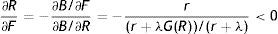
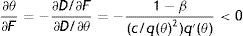
As (23) and (24) show, firing costs reduce both R and θ. The impact on R is due to the fact that destroying a job is more costly, whereas the impact on θ is because, once a job is created, firms will pay sooner or later the firing costs and this reduces the expected profit from a new job. To get the equilibrium impact we need to consider the overall impact of F, so we differentiate (12) and (14), respectively as B(R*,θ(R*,F),p,F,ω)=0 and D(θ*,R(θ*,F),F,ω)=0 and we get
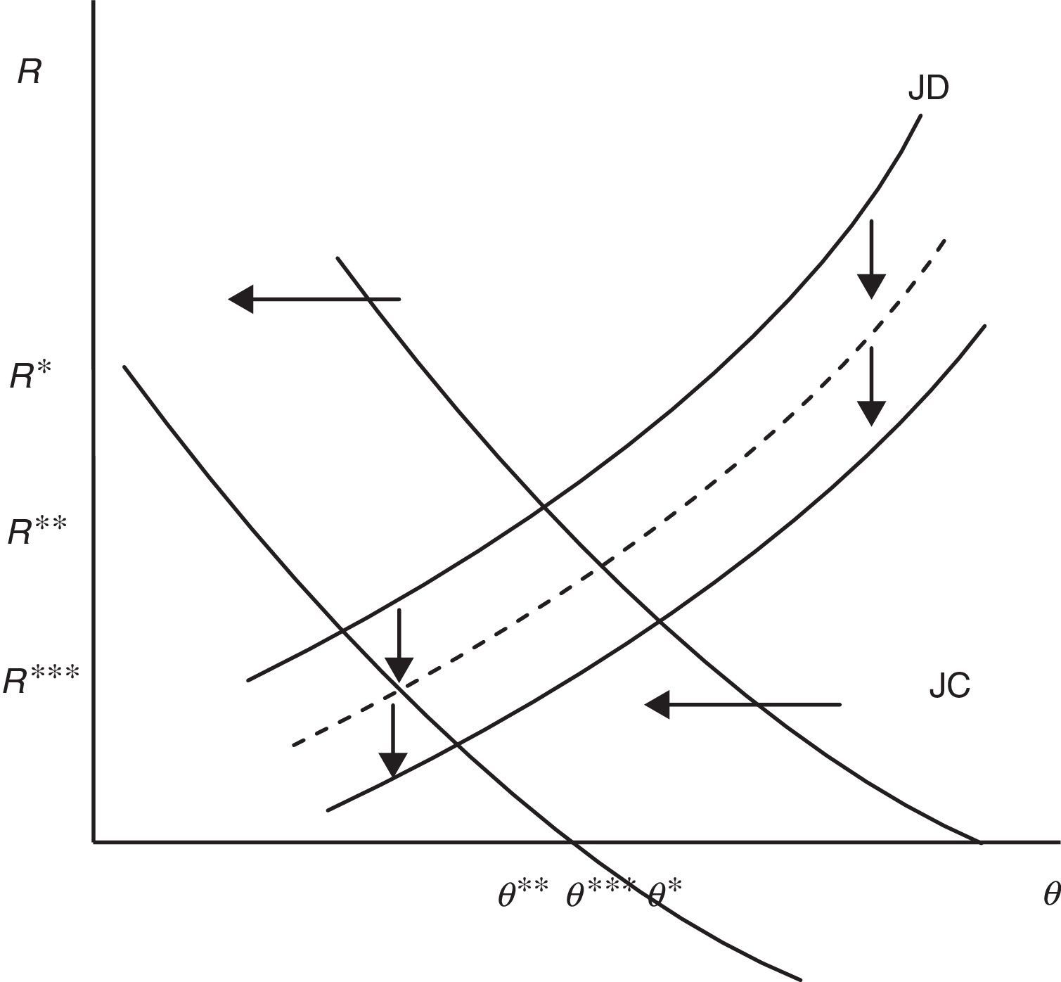
Therefore, in equilibrium firing costs reduce both job destruction and job creation. In particular, we can see that the equilibrium impact on job destruction (25) is even stronger than the initial impact (23), because higher firing costs reduce market tightness and in turn wage, thus less jobs are destroyed marginally (see (15) and (24)). On the other hand, the equilibrium impact on job creation (26) is weaker than the initial impact (24), because firing costs increase the duration of jobs and this partially attenuates the loss of the expected profit due to F (see (16) and (23)). The equilibrium impact is illustrated in Fig. 4, where higher F shifts JD down and JC left. As the figure shows, job destruction decreases unambiguously whereas the effect on job creation would seem ambiguous, but indeed we know from (26) that job creation decreases as well.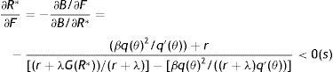

.")
Because of the symmetric impact on job creation and job destruction, the impact of firing costs on unemployment in matching models is usually ambiguous, as differentiation of (21) shows
The equilibrium impact on unemployment is illustrated in Fig. 5. Higher firing costs shift the Beveridge Curve in and rotate the job creation line clockwise, therefore the impact on unemployment is ambiguous, but vacancies decrease unambiguously.

So far, we considered p a parameter unaffected by firing costs and, basically, we obtained the same results of the previous literature without significant novelty. Nonetheless, in our model p is the endogenous component of labour productivity, thus now we regard it as endogenous and, in particular, we allow it to be affected by a change in F. Intuitively, we expect that firing costs affect in some way the behavioural component of productivity for different reasons. Firstly, as (7) and (8) show firing costs affect directly the actual and future wage. Moreover, they affect indirectly wage through the probability of finding a job (θq(θ)). Finally, they influence the probability of being fired (λG(R)), affecting the continuation value of (17).
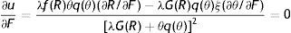
From (18) we have that the initial impact of firing costs on optimal productivity is null, that is

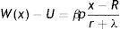
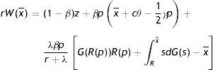
The economic intuition of this result is that firing costs have a negative effect on the outside wage and a positive effect on the inside wage, thus in expectations these two impacts on the permanent income of a new worker compensate, as showed by (17). This interpretation is made evident by the difference between (17) and the permanent income of a worker inside a match
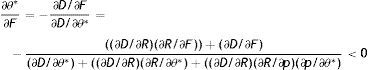
where firing costs certainly have a positive effect on wage. Therefore, all the effect of F on p should be induced by the impact on the other endogenous affecting the worker continuation value. In fact, as long as R and θ do not vary there is no change on the continuation value and the permanent income of a new worker, thus there should be no impact on labour productivity. To get the equilibrium impact we differentiate (18) as M(p*,R(θ,p*,F),θ(R,F),ω)=0 and we get the following:Proposition 1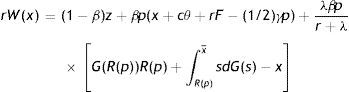

A higher level of EPL reduces the equilibrium labour productivity through the impact on reservation productivity and market tightness.6
The economic intuition of this result lies in the following argument. As (12) shows, labour productivity has a negative impact on reservation productivity through the production effect, therefore in the choice of the optimal p the production effect induces workers to choose marginally a higher p to reduce R and, in turn, the probability of being fired (λG(R)). Indeed, when we analyze the impact of firing costs on reservation productivity we can easily realize that the effect is of the same magnitude of the production effect. To see this point let multiply (12) by p and concentrate on the production effect and the firing costs effect, ignoring for a while the other elements

As (28) shows, the production effect is partially substituted by the firing costs effect in lowering R and thus a higher F, amplifying the relevance of the disutility effect, induces workers to choose marginally a lower p. Moreover, a higher F reduces also θ and consequently both outside and inside wage, again inducing workers to choose a lower p (see (24)). The equilibrium impact is illustrated in Fig. 6, when a higher F shifts RE down and PE left.

Considering p the endogenous component of productivity leads us to reassess the equilibrium impact of F on job creation and job destruction. In particular, now we differentiate (12) and (14), respectively as B(R*,θ(R*,F),p(R*,θ),F,ω)=0 and D(θ*,R(θ*,F,p(R,θ*)),F,ω)=0 and we get
from which we can easily establish the following results (29)>(25) and (30)<(26), summarized in the next Proposition:Proposition 2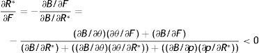
Compared to the standard equilibrium with p as a parameter of the model, in the equilibrium with endogenous labour productivity EPL reduces even more job destruction, but reduces less job creation.
The economic intuition of this result is that, as we have seen before (28), the presence of a more stringent protection legislation reduces the role of the production effect and amplifies that of the disutility-wage effect, leading to a lower labour productivity which decreases wages and, in turn, the optimal reservation productivity. Consequently, lower job destruction increases the expected duration of job and partially attenuates the loss of the expected profit due to higher firing costs, leading to a smaller reduction of job creation. The equilibrium impact on R and θ with endogenous labour productivity is illustrated in Fig. 7.
.")
In conclusion, regarding p as the endogenous component of productivity changes quantitatively the equilibrium impact of F on job creation and job destruction, but not the direction. However, firstly the extension of the model with endogenous labour productivity should be important per se, especially in the light of the recent empirical evidence on the impact of EPL on labour productivity. Moreover, as will be clear in the next section, considering p an endogenous object of the model turns out to be very much important for the quantitative exercise and, in particular, for the welfare analysis and consequent policy implications concerning EPL.
5Quantitative analysisIn this section we attempt a rough calibration of the model to evaluate quantitatively the impact of firing costs not only on labour market performance, but also on some measure of aggregate welfare. As standard in this literature, we adopt the following Cobb-Douglas matching function with constant returns to scale, usually the specification most appropriate to match the data on job creation (see e.g. Layard et al., 1991, for the UK; Blanchard and Diamond, 1989, for the US)
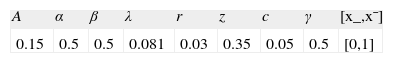
Furthermore, the distribution of the idiosyncratic component of productivity is taken uniform over the support [0,1],7 i.e. G(x)=(x−x_)/(x¯−x_)=x. Following the previous literature, the baseline parameters reported in Table 1 are set so as to match some typical features of the empirical data (e.g. Davis and Haltiwanger, 1992). To this extent, the parameters of the matching function are set as usual at A=0.15 and α=0.5. The workers’ bargaining power is set at β=0.5 equal to the elasticity of the matching function, so as to get constrained efficiency at least in the economy without firing costs (e.g. Hosios, 1990). To generate in the simulation reasonable job flows, the arrival rate of the idiosyncratic productivity shock is set λ=0.081 (see Mortensen and Pissarides, 1994). Similarly, the worker preference parameter governing the disutility of effort is set at γ=0.5, which induces an increasing disutility of effort but indeed generates reasonable values of labour productivity. Finally, in our simulation we consider a semester as the unit of time and, accordingly, we set the interest rate at r=0.03 (see e.g. Cahuc and Postel-Vinay, 2002).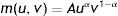
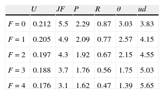
In order to assess the impact of firing costs on labour market performance, we compute8 different equilibriums of the model with F varying from 0 to 4. This should cover a significant range, from the laissez–faire case (F=0) to the substantial firing restrictions case (F=4), where firing costs are more than three times the semester wage (see e.g. for Italy Garibaldi, 2006). In Table 2 we report the equilibrium values of unemployment rate, job flows, labour productivity, reservation productivity, market tightness and unemployment spell duration for different levels of firing restrictions.
First, we can see that more stringent firing restrictions reduce significantly the equilibrium labour productivity. In particular, a level of firing costs equal to two times the semester wage (F=2) is enough to reduce labour productivity more than 10% respect to the laissez–faire case, whereas in the substantial firing restrictions case the reduction is even of the 30%. Similarly, firing costs reduce both reservation productivity and market tightness and, in turn, job flows. As we can see, job flows in the substantial firing restrictions case are less than 60% of those in the laissez–faire case. Nonetheless, as standard in these models (e.g. Mortensen and Pissarides, 1999a), the overall impact on unemployment is positive, because the impact on job destruction overcomes that on job creation. Interestingly, the difference in the level of job flows between the economy with low firing costs (5.5−4.9) and that with high firing costs (3.7−3.1), seems to match reasonably the real data in the U.S., the quintessential frictionless country, and the European countries, where notoriously firing restrictions are consistent. Finally, because of the decrease on job creation, higher firing costs increase significantly the unemployment spell duration. In particular, in the substantial firing restrictions case the unemployment duration increases more than 50% respect to the laissez–faire case.
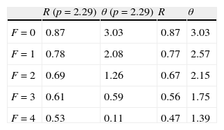
In Table 3 we show the equilibrium values of reservation productivity and market tightness in the model with p exogenous, along with their values for the complete specification. In particular, we set the exogenous productivity p at the equilibrium level get in the laissez–faire case (p=2.29) and we keep p fixed, regardless of the value of F. In this way we make clear what happen to job creation and job destruction when we allow labour productivity to adjust optimally to change in firing costs. As we can see, this numerical exercise confirms exactly the result of the qualitative analysis (see (29), (30) and Fig. 7). In particular, when we allow p to respond optimally to change in F, this leads to an even stronger reduction of the equilibrium reservation productivity, but to a smaller reduction of the equilibrium market tightness.
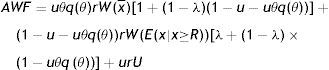
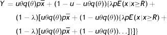
Finally, to assess the impact of firing costs on the well-being of the economy, we compute the value of different measures of aggregate welfare from the laissez–faire to the substantial firing restrictions case. In particular, we consider two main measures of aggregate welfare, the first concerning the production net of recruiting costs (Y−RC), the second the utility of agents (AWF). Our consistent measures of aggregate welfare in the economy are (see Appendix A)
where E(x|x≥R) indicates the conditional expectation of the idiosyncratic productivity x over the truncated distribution of the active units [R, x¯], that is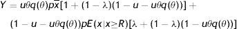
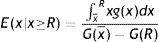
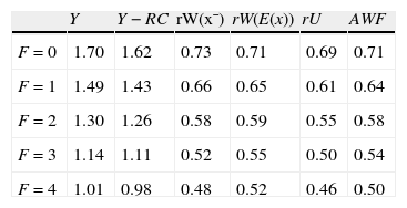
In Table 4 we report the equilibrium values of these two measures of aggregate welfare for different levels of firing restrictions. Along with these main measures of welfare, we report some other index of well-being in the economy, as the permanent income of unemployed and employed worker in different conditions.
As standard in the matching literature, firing restrictions reduce unambiguously all measures of aggregate welfare, regardless we think the well-being of the economy in terms of production or utility of agents.9 This is not surprising, since we know that under the restriction α=β the laissez–faire economy gets the constrained efficiency. More interesting is the size of the reduction of production. In particular, a middle level of firing restrictions is sufficient to yield a production 25% lower respect to the laissez–faire case, whereas in the substantial firing restrictions case the production is even 40% lower. Indeed, despite the negative impact of EPL on aggregate welfare being well known (see e.g. Cahuc and Postel-Vinay, 2002), such worrying reduction in production is not standard:Proposition 3 Compared to the standard matching model with p exogenous, in the equilibrium with endogenous labour productivity EPL reduces even more the aggregate welfare, regardless we consider the well-being of the economy in terms of production or aggregate utility.
Nonetheless, hidden under this result there is exactly the negative impact of firing restrictions on labour productivity, which not only reduces the total production of the economy, but also the surplus from job matches and, therefore, the utility of agents. Unsurprisingly, the inclusion in the analysis of this element enriches the picture of our model and, certainly, tells us an alarming result we should worry about.
6ConclusionThe matching model studied in this paper revealed that, indeed, the level of labour productivity in the economy can be influenced by labour market policies usually implemented by governments. Stimulated by the recent empirical evidence, we focused on EPL and showed that a higher level of firing restrictions partially substitute high labour productivity in reducing job destruction and this, consequently, brings down the optimal level of productivity. Furthermore, the response of productivity to EPL reasonably affects the level of production and, in fact, numerical simulation of the model showed that a higher level of firing costs should induce a consistent reduction on production, beyond the standard reduction found in the literature. Moreover, despite the reduction on the disutility of effort, higher EPL reduces unambiguously our measures of aggregate welfare (AWF), inducing a worsening on the well-being of both employed and unemployed workers. Therefore, in the light of the predominant role of labour productivity growth in driving the income growth in the last twenty years (OECD, 2003, 2007), the results of this paper bring a further element in support of the consolidated voice of the literature for a reduction of EPL especially in European countries.
To conclude, the extension of the endogenous labour productivity pursued in this paper allows us to rationalize within the already fruitful matching approach the well-established empirical evidence on the impact on EPL on labour productivity, which indeed assumes the appearance of a macro-stylized fact in the European economies and, thus, should be explained in a macro model of the labour market. On the other hand, the inclusion of the optimal workers’ response to political tools should represent a positive element for any other policy evaluation. In particular, including both optimal agents’ responses and market outcomes, the matching approach might turn out to be the ideal framework to address crucial questions usually analyzed in microeconomic contexts, but that certainly present significant macro implications.
The author would like to thank Robert Shimer, Roberto Cellini, Jeremy Lise, an anonymous referee and participants in various conferences and seminars for helpful comments and suggestions. The usual disclaimer applies.
There are different ways in which the permanent income equation (17) can be derived using the equilibrium conditions; we show one of these which allow us to establish different interesting relations.
First from the asset value of unemployed worker (4) we have that
From the asset value of employed worker (5) we have that
Evaluating (34) at the upper support of the price distribution and at the reservation productivity
Now subtracting (36) from (35) and using the reservation property W(R)=U we get
Substituting (33) in (37) we obtain
Similarly, subtract (36) from (34) to get
and now substitute (33) and use (38) to obtain
This expression interestingly says that when firing costs are low the permanent income of a generic worker is always lower than that of a new worker, the difference being due to the different level of the idiosyncratic productivity. However, when firing costs are high the advantage of being already inside a match, leading to a higher wage, overturns the relation in favour of the generic worker (see Table 4).
Finally, inserting (39) in the integral expression of the asset value of a new worker we get

and now using (37) and substituting the outside wage equation (7) gives us (17)
Similarly, inserting (39) in the asset value of the generic worker gives his permanent income.
In equilibrium there are (1−u) producing workers, who differ only for the level of the idiosyncratic productivity x. Among these uθq(θ) workers are in the first period of employment, therefore produce at the upper support of the price distribution x¯. Instead, the other (1−u−uθq(θ)) workers were employed already the previous period and indeed their level of x is not the same for all of them. In particular, a fraction λ faced a productivity shock and changed the level of x in a new value between x¯ and R, whereas the complement (1−λ) maintained the same level of the previous period. In turn, among these old workers maintaining the level of x, a fraction uθq(θ) entered two period ago and therefore produce at the upper support of the price distribution x¯, whereas the others (1−uθq(θ)) entered more than two period ago and indeed we should distinguish again between those who faced a productivity shock and those who not and so forth. Therefore, the total production is
As intuitive, the precise computation of the level of idiosyncratic productivity of producing workers in steady state is troubling, due to the recursive computation. Nonetheless, given that our aim is to evaluate the impact of firing restrictions on total production, it would be harmless to make an assumption to simplify the computation which affects in the same way the value of production between the laissez–faire and the substantial firing restriction case. Obviously, more an employed worker is old higher is the probability that he faced a productivity shock and changed his level of x. For simplicity, in (31) we assume that all workers older than two periods faced a productivity shock. Therefore, our measure of total production is
which after some easy algebra gives us (31).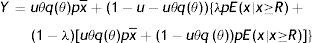
Moreover, to check if our assumption is really harmless for our purpose, we repeated a similar numerical exercise of Table 4 assuming that all workers older than three periods faced a productivity shock. As expected, we did not get any sizable difference on the impact of firing restrictions on output.
Similarly, the aggregate welfare function is the weighted sum of utility of the different workers in steady state, knowing that the utility of worker depends on the idiosyncratic component of productivity. Following the identical argument mentioned before, in equilibrium the aggregate welfare function is
which after some easy algebra gives us (32).
In particular, Dolado et al. (2011) work in a partial equilibrium environment with certainty, implying exogenous vacancy filling and job destruction rates. Moreover, they assume a linear disutility of effort (whereas here we work with an increasing disutility), which represents the unique component of productivity (that is, without any stochastic idiosyncratic component). Therefore, in their framework neither job destruction nor labour productivity of regular workers is affected by EPL.
Notice that this specification is without loss of generality, given that for the utility function below an additional parameter on the relation p=φe would not be identified, but only γ/φ2 would be identified.
The derivation of the inside and outside wage equations can be found in the working paper version (Lisi, 2010), which can be downloaded from http://www.demq.unict.it/db/Allegati/wp_2010_08_c1_merged.pdf.
At first sight, the S.O.C. for this maximization problem would depend on the value of parameters
However, for a very large set of values, indeed all the plausible ones, numerical computations unequivocally show that the condition ∂2rW(x¯)/∂p2<0 is respected.
A much more rigorous analysis of the transitional dynamics in this kind of models has been pursued in Pissarides (1985 or 1990) and can be found also in Pissarides (1990). However, here we follow the same line and arguments of Pissarides (2000).
At first sight, there might be an ambiguity on the denominator of (27). However, both graphical analysis and numerical computations with a large set of values, indeed the most plausible ones, unequivocally show that (27) is negative.
Usually, in the literature the idiosyncratic component of productivity x is an additive component of total price (p+x) and the distribution is taken uniform over [x_,x¯], with x_ being a negative number. However, the exogenous level of labour productivity p is fixed so that the total price is fairly everywhere positive (see e.g. Mortensen and Pissarides, 1994, 1999a,b). Differently, in our model we make a preference for the interpretation of the idiosyncratic component as a multiplicative component of total price (px), thus we need to adopt a positive support for the distribution (see Lilien, 1982; Blanchard and Diamond, 1989; Pissarides, 2000). Nonetheless, it is clear that both interpretations maintain the same mechanism underpinning the reservation productivity.
Fix point algorithm written in Matlab available under request by the author.
For what concern the welfare measure in terms of utility we should remember that we assumed risk neutral and impatient workers, which implies zero saving and full consumption. This is usually done in this literature in order to avoid to solving the consumption problem, so that we can work with the maximized Bellman equation to derive the steady-state of the model. Nonetheless, such limitation should be somewhat taken in mind when we think about the policy implications of our results.