


Mathematical models are often used to predict microbial growth in food products. An important class of these models involves the adaptation of classical sigmoid functions, such as the Gompertz and logistic functions. This study aimed to validate the use of the modified Richards model in various situations, which have not previously been tested. The model was obtained through solving a system of two differential equations and could be applied to both isothermal and non-isothermal environments. To test and validate this model, we used published datasets containing data for the growth of Pseudomonas spp. in fish products. The results obtained after fitting the model showed that it could be effectively used to describe and predict the Pseudomonas growth curves under various temperature regimens. However, the influence of the shape parameter on the growth curve is an issue that needs further evaluation.
The control of the processing, packaging, distribution, and storage conditions of many food products is of major importance for the assurance of food safety. The microbial stability of food is affected by several environmental factors such as temperature, pH, and water activity. These factors can undergo significant changes throughout the production chain, and food may become potentially unsafe due to the presence of spoilage and/or growth of pathogenic microorganisms.1,2 Consequently, the concentration of microorganisms should be continuously monitored during the transportation of raw products, until they reach their final destination. However, this task is virtually impossible to accomplish because enumerating microorganisms during different stages of food processing using traditional approaches is slow and expensive.3,4 Therefore, classical microbial evaluation, especially that of perishable foods, is of limited value for predictive purposes since these foods are consumed or sold before the results of microbiological tests become available.
The use of equations and mathematical models to predict microbial growth has been adopted in predictive microbiology. This quantitative area enables users to objectively estimate the effect of processing and storage operations on the microbiological safety and quality of food.5 The main models commonly applied in the above-mentioned field are the modified Gompertz model and the Baranyi model.6–10 The Baranyi model is thought to provide a better goodness-of-fit than the modified Gompertz equation.10,11 It should also be mentioned that the modified Gompertz model lacks a mechanistic basis and that the Baranyi model provides a biological interpretation for the duration of the lag phase.12
In addition to the above-mentioned issues, when one addresses quantitative microbial risk assessment, it is important to develop microbial growth models that take into account the influence of environmental changes on the behavior of selected pathogens along the food production and supply chain. In this respect, temperature changes during different stages of the production chain process are determinant factors affecting pathogen growth. Thus, the predictive models able to take into account the influence of temperature changes on microbial growth may contribute to the prediction of a food's shelf life and/or risk assessment when dealing with spoilage or pathogenic microorganisms.4,9,13
The main purpose of this study was to validate a mathematical model describing microbial growth in food products under conditions that had not been previously tested. To test the ability of the model to correlate with experimental data, six different isothermal datasets and four non-isothermal datasets pertaining to Pseudomonas spp. growth in fish products were selected from the literature. The adjustable parameters obtained were used to estimate the kinetic properties, such as the maximum specific growth rate and the duration of the lag phase of the microorganism under investigation.
Materials and methodsModel descriptionIn this study, the modified Richards model was tested for temperature profiles that had not been previously evaluated. It has already been shown that the model can be derived from a system of two differential equations.14 The first equation consists of the most elementary model building block describing microbial evolution15 and can be written as follows:
where N(t) represents the microbial load and μ(N) corresponds to the specific growth rate of the microorganism.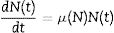
The second differential equation is related to the density dependence of the specific growth rate. The model is based on the usual assumption that μ(N) must be a decreasing function of the population, due to the accumulation of waste metabolites within the food environment. It is assumed, as represented by Eq. (2), that this decrease follows a power law:
where α is a positive parameter, which is assumed to depend on only the environmental conditions and not on the particular microorganism under study. The parameter m is a shape parameter and has no biological meaning.Isothermal environment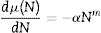
The analytical solution of the system of equations composed of Eqs. (1) and (2) at the initial conditions of N(0)=N0 and μ(N0)=μ0 in an isothermal environment is given by the following equation14:
Eq. (3) expresses the microbial load, N(t), as a function of the initial population, N0, the initial specific growth rate, μ0, the shape parameter, m, and the final population, Nf. It should be noted that, if m=−1, the equation is similar to a reparameterized version of the Gompertz model and if m=0, it is similar to a reparameterized version of the logistic equation. In this study, the population, N(t), was replaced by logN(t), which is similar to the modified Gompertz equation. Eq. (3) with m≠−1 is a reparameterized version of the Richards growth model,19 and for predictive microbiology purposes, it is known as a modified Richards model.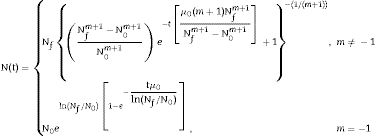
The application of Eq. (3) is useful for static environmental conditions (e.g., constant temperature). To obtain Eq. (3), the parameter α was replaced by a function of the other parameters of the model,14 as can be observed in Eq. (4). This procedure holds only for an isothermal environment. Therefore, this parameter is not used to fit the model to bacterial growth in an isothermal environment.
Non-isothermal environment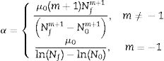
For situations that do not correspond to isothermal growth, Eqs. (1) and (2) should be used. Dynamic conditions, such as an increase or decrease of the temperature, require that a secondary model expressing the dependence of the growth rate on the temperature be used. In the current study, it was selected the Ratkowsky's square root model because it is largely adopted and validated in the field of predictive microbiology.16,17 Because the other parameters (μ0 and α) are not found in other models, another empirical secondary models for these parameters were included, and the resulting differential equation was numerically solved.
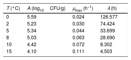
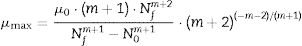
Biological parametersIn the present study, the following biological parameters were evaluated: the net logarithmic growth, A, the maximum specific growth rate, μmax, and the duration of the lag phase, λ. The parameters A and μmax can be obtained using Eqs. (5) and (6). It should be mentioned that μmax is estimated through the calculation of the inflection point of the growth curve. The duration of the lag phase was estimated using the procedure adopted by Buchanan and Cygnarowicz.18
Experimental data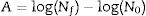
The bacterial growth data were collected from the literature20 and extracted from published curves using GetData Graph Digitizer 2.24 software (www.getdata-graph-digitizer.com). Six isothermal (0, 2, 5, 8, 10, and 15°C) and four non-isothermal datasets containing Pseudomonas spp. growth data in fish meat were selected. The non-isothermal temperature profiles used in this study correspond to sudden shifts in temperature and can be expressed by functions with if-statements, as follows:
Numerical methods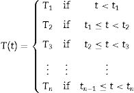
Fitting of the primary and secondary models to the experimental microbial growth data was performed using the fit function of the curve fitting toolbox available in the Matlab R2011b software, version 7.13 (MathWorks, Natick, MA, USA). This toolbox uses the nonlinear least squares method and the trust-region reflective of Newton's method. The initial estimate for each parameter of the model was obtained through a visual inspection of the curves.
The numerical solution of the differential equations for the non-isothermal growth curves was obtained with the ode23 function available in Matlab. The ode23 function is a general-purpose algorithm based on the Runge–Kutta method. This method can automatically adjust the computational step size to achieve a desired accuracy when numerically solving ordinary differential equations.
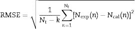
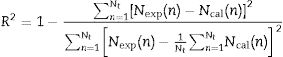
Statistical analysisThe performance of the model was evaluated using root mean square error, RMSE (Eq. (8)), and the coefficient of determination, R2 (Eq. (9)). In these expressions, Nexp stands for the experimental data, Ncal stands for the result predicted by the model, Nt represents the total number of experimental points, and k corresponds to the number of parameters in the model.
A comparison between the experimental values and the responses predicted by the non-isothermal mathematical model was carried out using the RMSE and the bias (BF) and accuracy factors (AF), which are given by Eqs. (10) and (11), respectively21:
ResultsIsothermal growth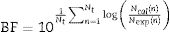
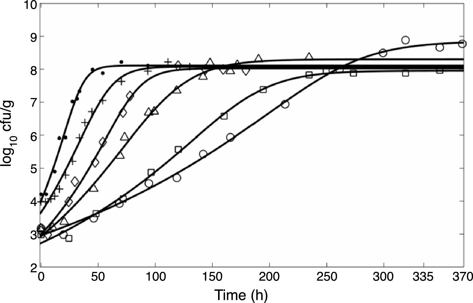
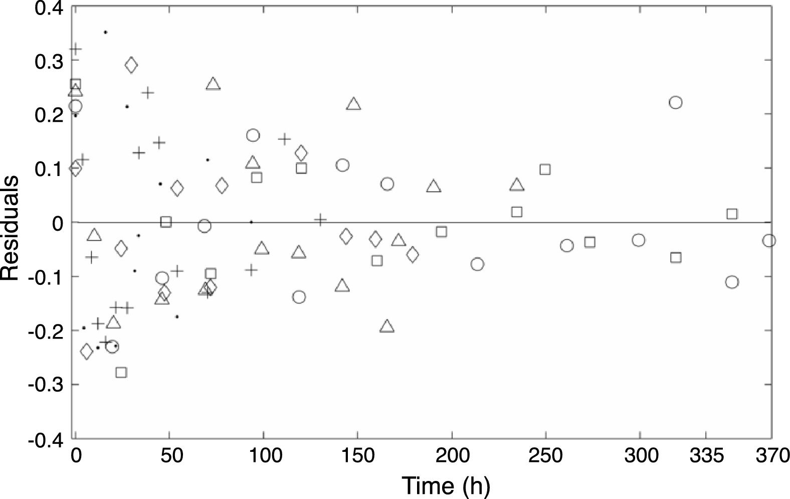
In the present study, the primary model given by Eq. (3) was fitted to the experimental data obtained at six different temperatures. The curves obtained are shown in Fig. 1. The residuals obtained after fitting the model are plotted in Fig. 2 and are shown to be approximately independent and normally distributed. However, it was observed for most of the temperatures studied that the initial log count was slightly underestimated relative to the experimental results.
 to the data for Pseudomonas spp. growth in fish obtained at (○) 0°C, (□) 2°C, (▵) 5°C, (♢) 8°C, (+) 10°C, and (●) 15°C.")
Fit of Eq. (5) to the data for Pseudomonas spp. growth in fish obtained at (○) 0°C, (□) 2°C, (▵) 5°C, (♢) 8°C, (+) 10°C, and (●) 15°C.
 to the experimental data generated at (○) 0°C, (□) 2°C, (▵) 5°C, (♢) 8°C, (+) 10°C, and (●) 15°C.")
Plot of the residuals obtained after the fit of Eq. (3) to the experimental data generated at (○) 0°C, (□) 2°C, (▵) 5°C, (♢) 8°C, (+) 10°C, and (●) 15°C.
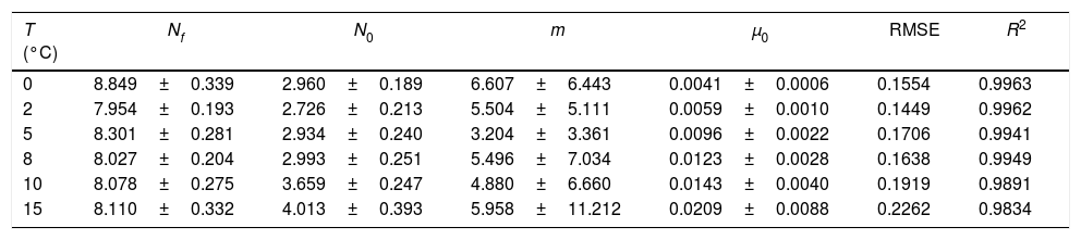
Table 1 shows the numerical values estimated for the model parameters within the 95% confidence limit, as well as the RMSE and R2 values. These values were obtained after fitting the mathematical model to the experimental data for the six temperatures investigated. The fit of the modified Richards model to the Pseudomonas spp. experimental data provided as good a performance as that of the four-parameter logistic model used in the original research,20 with an R2 greater than 0.983 and an RMSE lower than 0.226 log of colony forming units (CFU)/g, as shown in Table 1.
Summary of the model parameters and statistical indices obtained for isothermal growth for each temperature studied.
| T (°C) | Nf | N0 | m | μ0 | RMSE | R2 |
|---|---|---|---|---|---|---|
| 0 | 8.849±0.339 | 2.960±0.189 | 6.607±6.443 | 0.0041±0.0006 | 0.1554 | 0.9963 |
| 2 | 7.954±0.193 | 2.726±0.213 | 5.504±5.111 | 0.0059±0.0010 | 0.1449 | 0.9962 |
| 5 | 8.301±0.281 | 2.934±0.240 | 3.204±3.361 | 0.0096±0.0022 | 0.1706 | 0.9941 |
| 8 | 8.027±0.204 | 2.993±0.251 | 5.496±7.034 | 0.0123±0.0028 | 0.1638 | 0.9949 |
| 10 | 8.078±0.275 | 3.659±0.247 | 4.880±6.660 | 0.0143±0.0040 | 0.1919 | 0.9891 |
| 15 | 8.110±0.332 | 4.013±0.393 | 5.958±11.212 | 0.0209±0.0088 | 0.2262 | 0.9834 |
Some authors have reported the use of other empirical and semi-mechanistic models to fit the data obtained for Pseudomonas spp. growing in fish. Corradini and Peleg22 used a modified version of the logistic equation to model the same experimental datasets that were used here. They considered Y(t)=log[N(t)/N0] and included in the logistic equation a constant that satisfies the following conditions: at t=0, Y(t)=0 and as t→∞, Y(t)=constant. The empirical growth models adopted in the studies of Koutsoumanis20 and Corradini and Peleg22 were different modifications of the classical Verhulst model. Lee23 showed that the semi-mechanistic Baranyi model and the Huang model also provided an adequate description of Pseudomonas spp. growth. Both models include an adaptation function that describes the duration of the lag phase in the elementary differential equation (Eq. (1)). In the Baranyi model, the adaptation function quantifies the physiological state of the microbial cells,12 while in the Huang model the adaptation function is only an empirical expression (logistic function).24 Robazza et al.25 also used a semi-mechanistic model based on the Central Limit Theorem to model the same experimental data. This model provides a link between the physiological state of individual cells and the specific growth rate of the population.
Some other authors have also modeled the growth of Pseudomonas spp. in poultry9,26 and pork meat.2 The Baranyi and modified Gompertz models were fitted to the growth data of Pseudomonas spp. in poultry meat obtained under five isothermal conditions.9 Both models showed goodness-of-fit results close to what was expected for all of the datasets adopted, with the RMSE values lower than 0.1477 and the pseudo-R2 values greater than 0.9779. Li et al.2 studied Pseudomonas spp. growth in pork meat at six isothermal conditions and evaluated three primary models for data fitting to select the best one. The modified Gompertz, Baranyi and Huang models were used in the study, but no single model could provide a consistently preferable goodness-of-fit measure for all the growth data. Li et al.26 showed that the Baranyi model was more suitable than the Gompertz and Huang models for fitting the data for Pseudomonas spp. growth in chicken products under five different storage temperatures.
As shown in Table 1, the shape parameter m is statistically less stable than the other parameters. The results suggest that this parameter should be fixed prior to fitting the model to the data. Table 2 summarizes the results obtained for these parameters for each temperature adopted.
From the results presented in Table 2, it can be observed that the values obtained for the parameters, mainly μmax and λ, are different from those obtained in previous research using the same datasets.20 This result is not surprising, since the two studies used different mathematical models and different procedures for evaluation of the parameters. These results can also explain the overestimation of the duration of the lag phase. It can be confirmed by visual inspection of Fig. 1 that the results presented in Table 2 do not reproduce the actual values of the lag phase duration. However, the major drawback of the model is the m parameter. Since it cannot be estimated with confidence, small variations in this parameter can significantly change the values of the remaining parameters. Despite the good performance of the model, which is reflected in the coefficient of determination values presented in Table 1, there may be many combinations of the model parameters that can provide similar fits. As can be seen from Table 1, even for the small range of temperatures adopted (from 0°C to 15°C) in the present study, it was obtained a large variation in the values of the parameter m (over 100%, ranging from 3.204 to 6.607). Thus, it is difficult to establish a single value a priori to this parameter. Some commonly used models, like the Baranyi model, arbitrarily fixes this value as being equal to 1.7,8 However, from the results presented in Table 1, it hardly can be said that this value is the best option for the data sets analyzed. Therefore, it was opted not to establish a single value to m and fit the resulting equation to experimental data. Instead, the focus consisted in evaluating the behavior of m in a range of conditions as a case study for a systematic use of the model in future studies.
Non-isothermal growthTo evaluate non-isothermal growth, it was considered that α and μ0 could be expressed as functions of the temperature in Eq. (2). Thus, the solution of this equation provides the following result:
Insertion of Eq. (12) into Eq. (1), with the temperature profile considered in terms of α(T) and μ0(T), provides a differential equation that must be numerically solved to generate predictions for non-isothermal growth. The temperature dependence of these parameters was obtained by fitting linear (μ0) and square-root (α) models to the data from Table 1. These expressions were empirically selected and have no special meaning. The results can be expressed by Eqs. (13) and (14):


The other parameters of the model (m and Nf) did not significantly change with temperature. Thus, the mean values of m and Nf were determined to be 5.275 and 8.220, respectively. Since these results were included in the confidence intervals of these parameters for all the temperatures studied, it was assumed that they could be safely used for the fitting process. In other words, the assumption is that under non-isothermal conditions the momentary growth rate coincides with the isothermal growth rate at the same temperature at a time that corresponds to the momentary growth level, as discussed by Corradini and Peleg.22
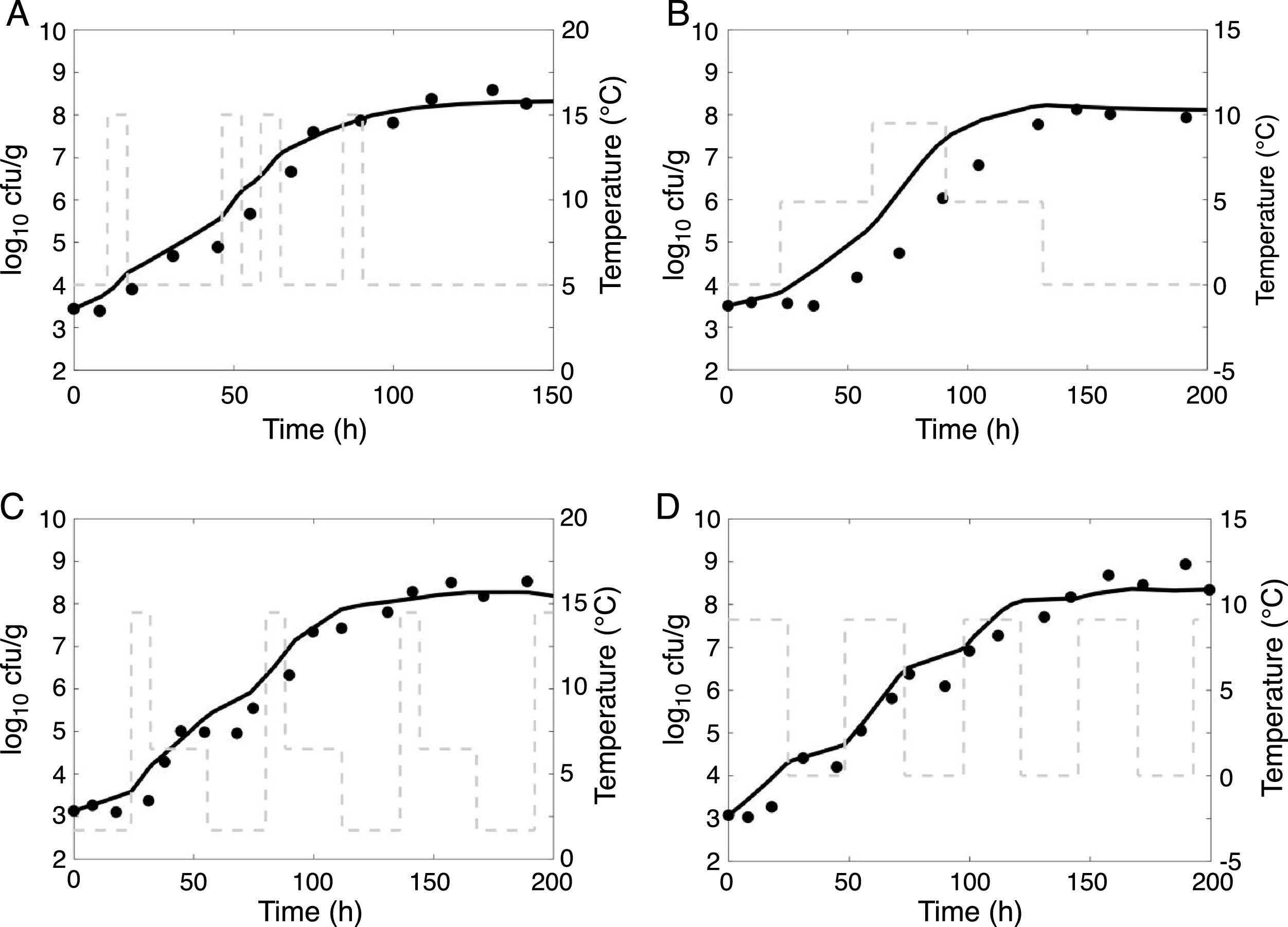
Fig. 3 shows the predictions supplied by the model for the non-isothermal conditions. The dots represent experimental data, the curves represent the fits obtained by the model, and the gray lines correspond to the temperature profiles.
 temperature profile 1, (B) temperature profile 2, (C) temperature profile 3 and (D) temperature profile 4.")
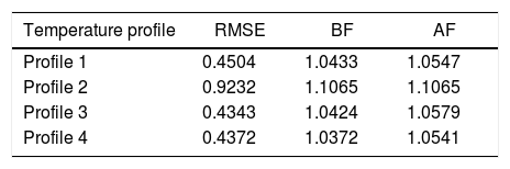
Table 3 presents the results obtained for the statistical indices adopted in the present study.
DiscussionGospavic et al.9 observed a good agreement in the maximum specific growth rates between the modified Gompertz and Baranyi models, but the duration of the lag phase did not agree as well. These authors explained the difference based on the confidence intervals computed for the model parameters. For the modified Gompertz model, the confidence intervals for the parameters were larger than those obtained for the Baranyi model, indicating that the lag phase parameters obtained by the Baranyi model were determined with a higher confidence than the ones obtained by the modified Gompertz model. Regarding the model evaluated in the present study, it can be observed from the results presented in Table 1, it can be observed that the parameters with a direct biological interpretation, N0 and Nf are more stable and can be estimated with higher confidence. The parameter μ0 is related to the initial specific growth rate which is close to zero at the lag phase. It can be seen that this parameter is less stable for higher temperatures which can be ascribed to the smaller duration of the lag phase.
From analysis of the data presented in Table 3, it can be concluded that, in general, the modified Richards model showed good agreement with the experimental data, as demonstrated by the BF values ranging from 1.0372 to 1.1065 and the AF values ranging from 1.0541 to 1.1065. Compared to the logistic model used for the same datasets in previous research,20 the performance of the modified Richards model was better,20 since the statistical indices were, in general, closer to those in the present study. Based on the prediction parameters (BF and AF), the performance of the modified Richards model was similar to that of the Baranyi and Huang semi-mechanistic models23 and Central Limit Theorem model.25
The Baranyi model furnished BF values that ranged from 1.023 to 1.083 and AF values from 1.053 to 1.087, while the Huang model showed BF values from 1.009 to 1.081 and AF values that ranged from 1.044 to 1.089. The model based on the Central Limit Theorem furnished BF values that ranged from 0.99 to 1.13 and AF values from 1.04 to 1.13. These ranges of BF and AF values obtained by the non-isothermal models are considered acceptable. It was demonstrated that the modified Richards model had a slight discrepancy compared with the experimental data, but only for Profile 2. Similar results were obtained for other models using the same experimental dataset.20,23,25
Bruckner et al.4 developed a dynamic model by combining the modified Gompertz model as the primary model and the Arrhenius equation as the secondary model to predict the growth of Pseudomonas spp. in fresh pork and fresh poultry meats. For the validation of the model under non-isothermal conditions, nine dynamic temperature scenarios were used. In this study, BF ranged from 0.87 to 1.01 for pork and from 0.89 to 1.04 for poultry, and AF varied between 1.05 and 1.24 for pork and between 1.05 and 1.16 for poultry. Koutsoumanis et al.27 developed and validated a microbial model for Pseudomonas growth in ground meat (beef and pork) under dynamic temperature conditions. The Baranyi model was used to predict food spoilage and the growth of the bacterium under four different fluctuating temperature profiles, with temperature shifts from 0 to 20°C. The performance of the model was evaluated by the percentage of relative errors (% RE) and 93.3% of the pseudomonad predictions fell within the −10 to 10% RE zone for all the scenarios tested, while none fell outside the −20 to 20% RE zone.27
The different predictive abilities of the models for non-isothermal profiles are related to the goodness-of-fit of the model parameters with the temperature and to the behavior of bacteria when subjected to environmental stress.13,27 The lack of understanding of the physiology of bacteria when subjected to stress conditions, such as temperature shifts, is still an obstacle to improving the growth models and obtaining better predictions.
ConclusionsIn the present study, a modified version of the Richards growth model was evaluated for describing microbial growth in food products. The model is composed of four adjustable parameters and provided accurate fits for isothermal environments. In addition, it was validated for non-isothermal environments. It consists in a different approach to describe microbial growth in a non-isothermal environment, since it takes into account the influence of the shape parameter on the growth curve. Since the model can be considered a reparameterization of the Richards growth model that encompasses both logistic and Gompertz growth models, it can be expected that the model, in general, would provide an accurate fit to the experimental data. However, there is a shape parameter included in the mathematical equations that does not have a biological meaning and exhibits an irregular behavior in nonlinear regression. Therefore, further work is needed to study the properties of the model and the behavior of its parameters in order for the model to be applied confidently and safely in predictive microbiology.
Conflicts of interestThe authors declare no conflicts of interest.
We would like to thank the Conselho Nacional de Desenvolvimento Científico e Tecnológico (CNPq) for financial support (Process 484037/2013-7).