

Los productos que proveen estimaciones de lluvia derivadas de satélites son útiles para el monitoreo tanto ambiental como de sequías, y permiten además afrontar el problema de las observaciones derivadas de estaciones pluviométricas mal distribuidas, siempre y cuando su precisión sea conocida. Venezuela es altamente vulnerable a eventos climáticos extremos como sequías extensivas y crecientes rápidas, por lo tanto conocer las debilidades y fortalezas de las estimaciones de lluvias derivadas de satélites resulta útil para la planificación de los recursos hídricos. Las estimaciones mensuales de lluvia derivadas del producto Climate Hazards Group InfraRed Precipitation with Stations (CHIRPS v.2) son contrastadas con los registros proveniente de estaciones climáticas (1981-2007), empleando métricas numéricas para evaluar su desempeño en la estimación de la cantidad de lluvia, y métricas categóricas para evaluar su capacidad de detección de eventos de lluvia. Los análisis aplicados consideran diferentes categorías de lluvia, la estacionalidad y el contexto espacial. Los resultados muestran que el producto CHIRPS v.2 sobreestima (subestima) los valores más bajos (altos) de lluvia, aunque en la mayoría de las métricas de habilidad muestra un buen desempeño. Este producto consigue un mejor desempeño durante la estación lluviosa (abril-septiembre), pero sobreestima significativamente la frecuencia de los eventos de lluvias. También muestra mejor desempeño global en regiones planas abiertas (p. ej., Los Llanos), donde la precipitación es influida por la actividad de la zona de convergencia intertropical y los sistemas convectivos locales.
Satellite-derived rainfall products are useful for both drought and environmental monitoring, and they also allow for tackling the problem of sparse, unevenly distributed and erratic rain gauge observations provided. their accuracy is well known. Venezuela is a country highly vulnerable to extreme weather events such as extensive droughts and flash floods; therefore, an understanding of the strengths and weaknesses of satellite-based rainfall products is useful for the planning of water resources. Using numerical metrics in order to evaluate performance, monthly rainfall estimates, from the Climate Hazards Group InfraRed Precipitation and Stations (CHIRPS v.2) product, are compared to gauge data from the 1981-2007 interval and categorical metrics for assessing rain-detection skills. The analysis was performed considering different rainfall categories, seasonality, and spatial context. The results show that the satellite product CHIRPS v.2 overestimates (underestimates) low (high) monthly rainfall values; although on the majority of numerical metrics of skill shows a good performance. This product, on the other hand, achieves better performance during the rainy season (April-September), significantly overestimating, however, the rainfall-events frequency. The product also shows best overall performance over flat and open regions (e.g., Los Llanos), where precipitation is influenced by the Intertropical Convergence Zone activity and local convective systems.
Venezuela is a tropical country located in northern South America with a total area of 916 445 km2; about 96% of this area is land. Although most of Venezuelan economy is based on the petroleum market, about 25% of the Venezuelan land area is dedicated to rain-fed farming (Betancourt, 2001; Weyland, 2002). Rain-fed agriculture is the dominant farming system in the Central Plains of Venezuela. This region also contains the largest reservoirs in the country, which supply water to the biggest and industrialized cities, which are located mainly in the northern region (Berroterán and Zinck, 2000; Sanso and Guenni, 2000; Mora and Rojas, 2007; Paredes et al., 2014).
The Caroni river hydropower reservoirs system (known as the Guri dam) is the most important energy source nationwide. Situated in the southeast region, it provides nearly 70% of the national hydropower demand (Bartle, 2002; Bautista, 2012). Both the central and southeast regions are characterized by high rainfall variability (Paredes and Guevara, 2000; Paredes et al., 2014). This climatological feature favors the occurrence of prolonged droughts whose impacts can negatively affect the agricultural and electrical sectors (Easterling et al., 2000; Blunden and Arndt, 2015). For instance, the rainfall deficit during 2010 (Millano and Paredes, 2013) and 2015 revealed that the hydropower and agriculture sectors are highly sensitive to extreme drought conditions in Venezuela (Grimm and Tedeschi, 2009); consequently, rainfall measurement and monitoring play an important role in rainfall-linked risk management.
Rainfall monitoring is of remarkable importance for drought-prone and flood-prone regions (Xie and Arkin, 1997; Kogan, 1998; Hong et al., 2007). Therefore, there is an increasing need for accurate rainfall-based products for different applications, such as agricultural monitoring and water resources management in remote areas (Boken et al., 2005; Toté et al., 2015). In Venezuela, conventional rain gauges have been the main source of rainfall data (Paredes and Guevara, 2010). However, most of the rain gauge networks currently available are inadequate to produce reliable rainfall analysis, largely due to their scarce spatial coverage, the high-proportion of missing data, and short-length records (Guenni et al., 2008; Vila et al., 2009; Rozante et al., 2010).
Satellite-based rainfall estimates may provide plentiful information with spatio-temporal high-resolution over widespread regions where conventional rainfall data are scarce or absent (Su et al., 2008; Li et al., 2010). However, these estimates have several limitations (e.g., significant uncertainty), because none of the satellite sensors detect rainfall as such and the relationship between observations and precipitation is based on one or several proxy variables (Wu et al., 2012; Toté et al., 2015).
Algorithms to estimate rainfall from satellite observations are based either on thermal infrared (TIR) bands (from which cloud-top temperature can be inferred), or on passive microwave (PMW) sensors. The TIR-based approach takes into account the cold cloud duration (CCD), which is the time interval that a temperature pixel is below a certain threshold. This technique assumes that rainfall and CCD are linearly correlated (Kidd et al., 2003; Joyce et al., 2004). The PMW-based approach takes advantage of the fact that microwaves can penetrate clouds to explore their internal properties through the interaction of raindrops with the radiation field. In fact, the pattern of absorption/scattering of incident radiation provides information about atmospheric liquid water content and rainfall intensity (Kummerow et al., 2001).
Several studies show that TIR-based rainfall estimates may have a large uncertainty when some types of cold or warm clouds are present. This is the case of cirrus clouds, which are frequently confused with convective clouds such as cumulonimbus that have similar brightness; only cumulonimbus may produce rain (Grimes, 2008; Thiemig et al., 2013). Similarly, the PM-based rainfall estimates have a marked bias in the presence of warm orographic rains, and of very cold surfaces like those found in mountain-tops covered by ice, which can be interpreted as precipitation (Toté et al., 2015). In general, PMW-based algorithms show better performance than TIR-based techniques for instantaneous rain over well-defined geographic regions while for estimates, over longer periods, the TIR outperforms PMW algorithms (Kidd, 2001). To deal with these technical limitations, the more recent satellite-based rainfall products combine multiple data sources as TIR/PMW-based rainfall data sets coupled with in situ precipitation observations and/ or numerical model rainfall fields in order to improve the accuracy of these products (Joyce et al., 2004). TIR-PMW combined rainfall products from satellites are the latest in the series of rain products that have evolved over four decades.
At present, there is a wide variety of satellite-based rainfall products derived from multiple data sources. Climate Hazards Group InfraRed Precipitation with Stations (CHIRPS) is a relatively new rainfall product with high temporal and spatial resolution, and is based on multiple data sources. The CHIRPS product was developed by the U.S. Geological Survey Earth Resources Observation and Science Center in association with the Santa Barbara Climate Hazards Group at the University of California.
The CHIRPS product requires two steps for its operational production: (i) Pentadal rainfall estimates (five-day rainfall) are created from Cold Cloud Duration-based satellite data, which are obtained from regression models, and calibrated by using TMPA 3B42 pentadal precipitation; these estimates are expressed as a percentage of normal precipitation by dividing the estimated values for regression models by their long-term averages (this outcome is named CHIRP). (ii) In-situ observations from stations are blended with the CHIRP data in order to produce CHIRPS (Toté et al., 2015).
Monthly precipitation climatology used in the first step (named CHPclim) is obtained from the Agromet Group of the Food and Agriculture Organization of the United Nations (FAO) and the Global Historical Climate Network (GHCN); both are re-sampled to a common 0.05° grid by applying a moving window regression at local level and by considering several predictors drawn from the satellite fields and elevation and slope. The CHIRPS station stream processing incorporates data from public data streams (such as the GHCN monthly, GHCN daily, among others), and several private archives. The CHIRPS station blending procedure is a modified inverse-distance weighting algorithm. At this point, the CHIRP defines a local de-correlation distance, which is the distance where the estimated point-to-point correlation is zero. To generate these values, time series of CHIRP data are used to calculate the average correlation at a distance of 1.5° for each grid cell. This correlation combined with the assumption that the expected correlation is 1 when distance is 0, allows for estimation of a de-correlation slope, which is used in turn to estimate the zero-correlation distance. The correlation structure evolves in space and time tending to be stronger in areas of heavy well-organized convection (Funk et al., 2014)
The satellite-based rainfall estimates adjustment vs. rain gauge observations can increase the accuracy of estimated rainfall values. This operational procedure requires a rain gauge network with an appropriate spatial coverage and records of high quality to perform an adequate calibration and validation (Ebert et al., 2007). The assessment of satellite-based rainfall data is a key aspect; several performance indexes support the choice of most adequate rainfall-based products for certain applications; e.g., drought early warning, environmental monitoring or flood forecasting (Sorooshian et al., 2000). Most validation studies have been carried out in the African Sahel (Laurent et al., 1998; Nicholson et al., 2003), southeastern Africa (Toté et al., 2015), Brazil (Negri et al., 2002; Franchito et al., 2009), and Colombia (Dinku et al., 2010), among others countries. Despite its great potential for large-scale environmental monitoring, the CHIRPS product reliability has not been analyzed in detail in the case of the Venezuelan territory.
The aim of this article is to evaluate satellite-derived monthly rainfall estimates from the CHIRPS product for Venezuela, by comparing the CHIRPS-based rainfall estimates against rain gauge observations supplied by the Venezuelan meteorological and hydrological institute. The rainfall estimates for different rainfall categories and their variations within a temporal and spatial context is emphasized in this study. The CHIRPS product was chosen for its high spatial and temporal resolution and its free access. Specific questions are addressed here as to how the CHIRPS-based rainfall estimates can be compared to the gauge data for different rainfall categories, over the seasonal and spatial context.
This article is organized as follows: section 2 gives a short description of the study area; the data sets used are briefly described in section 3; the more relevant statistical methods are detailed in section 4; and section 5 comprises a discussion of the more notable results. Finally, conclusions are summarized in section 6.
2Study areaVenezuela is located between 73-60° W, 1-12° N with a tropical climate characterized by a warm and hot rainy season from April to September and a relatively cool and dry season from October to March. Annual mean rainfall varies from north to south and from the Caribbean coast to the highlands due mainly to orographic factors, which induce a spatial pattern with a wetter region in the southeast and a semiarid region along the northwest coast (Pulwarty et al., 1992; Peterson and Haug, 2006).
The synoptic-scale weather system over most of the country is controlled by the Intertropical Convergence Zone (ITCZ), except for the production of rainfall along the Venezuelan coastal region, which is influenced primarily by the tropical disturbances occurring off the coast of northwestern Africa. Furthermore, subtropical fronts and tropical temperate troughs may favor the occurrence of heavy inland rainfall at any time of the year (Pulwarty et al., 1992; Lyon, 2003; Guenni et al., 2008).
The rainfall regime can be affected by El Niño-Southern Oscillation (ENSO). Generally, the cool phase of ENSO is linked to wetter conditions above the average, whereas the warm phase of ENSO is related to drought conditions (Acevedo et al., 2001; Paredes and Guevara, 2010; Pérez, 2012; Peñaloza-Murillo, 2014). Recently, most significant climate events have been severe droughts, such as those of 2009/10, 2013/14 and early 2015 in large parts of central-northern Venezuela, and heavy rainfall in early June 2015, which induced flash floods and landslides in the Venezuelan Andes.
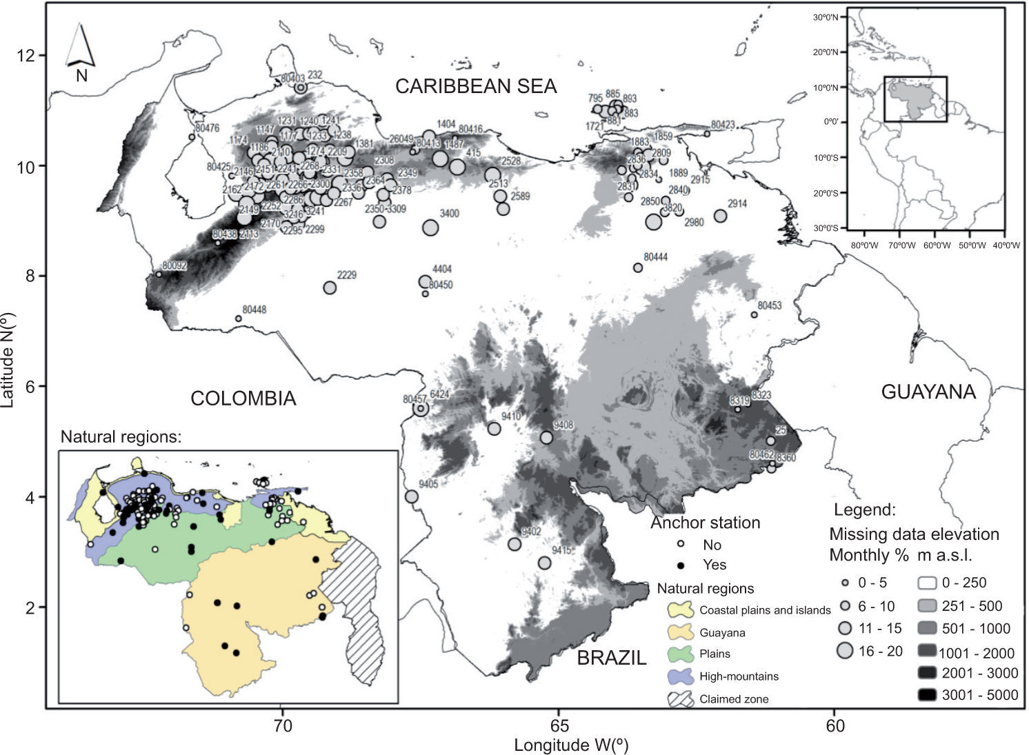
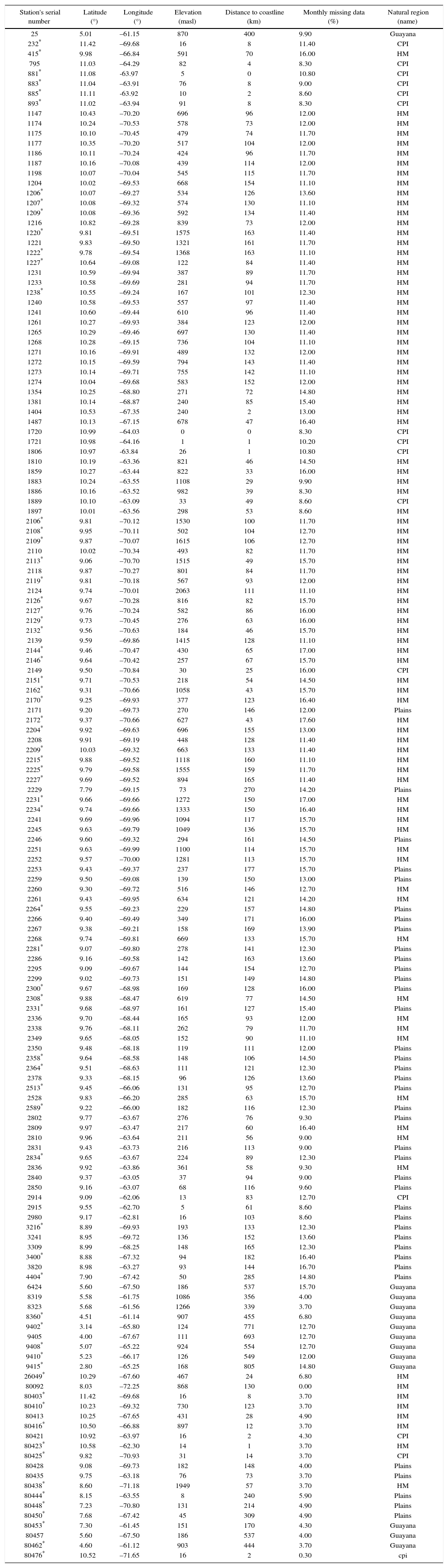
3Data3.1Gauge-based rainfall dataMonthly rain gauge observations were provided by the Instituto Nacional de Meteorología e Hidrología (INAMEH; available online at http://www.inameh.gob.ve/mensual/) and the Servicio de Meteorología de la Aviación Militar Venezolana (SEMETAVIA). The quality of this data, at each station and month, was previously verified based on the criterion of monthly mean ±3.5 standard deviations. Values outside this threshold and duplicated values of adjacent months were coded as missing data (Chapman, 2000). The monthly rainfall time series with more than 20% missing data were also omitted. A number of 154 stations were selected with these criterions whose monthly rainfall time series covered the period form 1981-2007 (Fig. 1, Table I).
 and by Venezuela's natural regions. Circles denote the location of selected rain gauges with sizes indicating the monthly percentage of missing data per station for the period 1981-2007. Numbers indicate the station ID.")
Terrain elevation in Venezuela. Top-right panel shows the location of Venezuela in South America. Bottom-left panel shows selected rain gauges location classified by station type (anchor or non-anchor) and by Venezuela's natural regions. Circles denote the location of selected rain gauges with sizes indicating the monthly percentage of missing data per station for the period 1981-2007. Numbers indicate the station ID.
Geographical and other information of selected rain gauges for the period 1981-2007.
| Station's serial number | Latitude (°) | Longitude (°) | Elevation (masl) | Distance to coastline (km) | Monthly missing data (%) | Natural region (name) |
|---|---|---|---|---|---|---|
| 25 | 5.01 | –61.15 | 870 | 400 | 9.90 | Guayana |
| 232* | 11.42 | –69.68 | 16 | 8 | 11.40 | CPI |
| 415* | 9.98 | –66.84 | 591 | 70 | 16.00 | HM |
| 795 | 11.03 | –64.29 | 82 | 4 | 8.30 | CPI |
| 881* | 11.08 | -63.97 | 5 | 0 | 10.80 | CPI |
| 883* | 11.04 | –63.91 | 76 | 8 | 9.00 | CPI |
| 885* | 11.11 | -63.92 | 10 | 2 | 8.60 | CPI |
| 893* | 11.02 | –63.94 | 91 | 8 | 8.30 | CPI |
| 1147 | 10.43 | –70.20 | 696 | 96 | 12.00 | HM |
| 1174 | 10.24 | –70.53 | 578 | 73 | 12.00 | HM |
| 1175 | 10.10 | –70.45 | 479 | 74 | 11.70 | HM |
| 1177 | 10.35 | –70.20 | 517 | 104 | 12.00 | HM |
| 1186 | 10.11 | –70.24 | 424 | 96 | 11.70 | HM |
| 1187 | 10.16 | –70.08 | 439 | 114 | 12.00 | HM |
| 1198 | 10.07 | –70.04 | 545 | 115 | 11.70 | HM |
| 1204 | 10.02 | –69.53 | 668 | 154 | 11.10 | HM |
| 1206* | 10.07 | –69.27 | 534 | 126 | 13.60 | HM |
| 1207* | 10.08 | –69.32 | 574 | 130 | 11.10 | HM |
| 1209* | 10.08 | –69.36 | 592 | 134 | 11.40 | HM |
| 1216 | 10.82 | –69.28 | 839 | 73 | 12.00 | HM |
| 1220* | 9.81 | –69.51 | 1575 | 163 | 11.40 | HM |
| 1221 | 9.83 | –69.50 | 1321 | 161 | 11.70 | HM |
| 1222* | 9.78 | –69.54 | 1368 | 163 | 11.10 | HM |
| 1227* | 10.64 | –69.08 | 122 | 84 | 11.40 | HM |
| 1231 | 10.59 | –69.94 | 387 | 89 | 11.70 | HM |
| 1233 | 10.58 | –69.69 | 281 | 94 | 11.70 | HM |
| 1238* | 10.55 | –69.24 | 167 | 101 | 12.30 | HM |
| 1240 | 10.58 | –69.53 | 557 | 97 | 11.40 | HM |
| 1241 | 10.60 | –69.44 | 610 | 96 | 11.40 | HM |
| 1261 | 10.27 | –69.93 | 384 | 123 | 12.00 | HM |
| 1265 | 10.29 | –69.46 | 697 | 130 | 11.40 | HM |
| 1268 | 10.28 | –69.15 | 736 | 104 | 11.10 | HM |
| 1271 | 10.16 | –69.91 | 489 | 132 | 12.00 | HM |
| 1272 | 10.15 | –69.59 | 794 | 143 | 11.40 | HM |
| 1273 | 10.14 | –69.71 | 755 | 142 | 11.10 | HM |
| 1274 | 10.04 | –69.68 | 583 | 152 | 12.00 | HM |
| 1354 | 10.25 | –68.80 | 271 | 72 | 14.80 | HM |
| 1381 | 10.14 | –68.87 | 240 | 85 | 15.40 | HM |
| 1404 | 10.53 | –67.35 | 240 | 2 | 13.00 | HM |
| 1487 | 10.13 | –67.15 | 678 | 47 | 16.40 | HM |
| 1720 | 10.99 | –64.03 | 0 | 0 | 8.30 | CPI |
| 1721 | 10.98 | –64.16 | 1 | 1 | 10.20 | CPI |
| 1806 | 10.97 | -63.84 | 26 | 1 | 10.80 | CPI |
| 1810 | 10.19 | –63.36 | 821 | 46 | 14.50 | HM |
| 1859 | 10.27 | –63.44 | 822 | 33 | 16.00 | HM |
| 1883 | 10.24 | –63.55 | 1108 | 29 | 9.90 | HM |
| 1886 | 10.16 | –63.52 | 982 | 39 | 8.30 | HM |
| 1889 | 10.10 | –63.09 | 33 | 49 | 8.60 | CPI |
| 1897 | 10.01 | –63.56 | 298 | 53 | 8.60 | HM |
| 2106* | 9.81 | –70.12 | 1530 | 100 | 11.70 | HM |
| 2108* | 9.95 | –70.11 | 502 | 104 | 12.70 | HM |
| 2109* | 9.87 | –70.07 | 1615 | 106 | 12.70 | HM |
| 2110 | 10.02 | –70.34 | 493 | 82 | 11.70 | HM |
| 2113* | 9.06 | –70.70 | 1515 | 49 | 15.70 | HM |
| 2118 | 9.87 | –70.27 | 801 | 84 | 11.70 | HM |
| 2119* | 9.81 | –70.18 | 567 | 93 | 12.00 | HM |
| 2124 | 9.74 | –70.01 | 2063 | 111 | 11.10 | HM |
| 2126* | 9.67 | –70.28 | 816 | 82 | 15.70 | HM |
| 2127* | 9.76 | –70.24 | 582 | 86 | 16.00 | HM |
| 2129* | 9.73 | –70.45 | 276 | 63 | 16.00 | HM |
| 2132* | 9.56 | –70.63 | 184 | 46 | 15.70 | HM |
| 2139 | 9.59 | –69.86 | 1415 | 128 | 11.10 | HM |
| 2144* | 9.46 | –70.47 | 430 | 65 | 17.00 | HM |
| 2146* | 9.64 | –70.42 | 257 | 67 | 15.70 | HM |
| 2149 | 9.50 | –70.84 | 30 | 25 | 16.00 | CPI |
| 2151* | 9.71 | –70.53 | 218 | 54 | 14.50 | HM |
| 2162* | 9.31 | –70.66 | 1058 | 43 | 15.70 | HM |
| 2170* | 9.25 | –69.93 | 377 | 123 | 16.40 | HM |
| 2171 | 9.20 | –69.73 | 270 | 146 | 12.00 | Plains |
| 2172* | 9.37 | –70.66 | 627 | 43 | 17.60 | HM |
| 2204* | 9.92 | –69.63 | 696 | 155 | 13.00 | HM |
| 2208 | 9.91 | –69.19 | 448 | 128 | 11.40 | HM |
| 2209* | 10.03 | –69.32 | 663 | 133 | 11.40 | HM |
| 2215* | 9.88 | –69.52 | 1118 | 160 | 11.10 | HM |
| 2225* | 9.79 | –69.58 | 1555 | 159 | 11.70 | HM |
| 2227* | 9.69 | –69.52 | 894 | 165 | 11.40 | HM |
| 2229 | 7.79 | –69.15 | 73 | 270 | 14.20 | Plains |
| 2231* | 9.66 | –69.66 | 1272 | 150 | 17.00 | HM |
| 2234* | 9.74 | –69.66 | 1333 | 150 | 16.40 | HM |
| 2241 | 9.69 | –69.96 | 1094 | 117 | 15.70 | HM |
| 2245 | 9.63 | –69.79 | 1049 | 136 | 15.70 | HM |
| 2246 | 9.60 | –69.32 | 294 | 161 | 14.50 | Plains |
| 2251 | 9.63 | –69.99 | 1100 | 114 | 15.70 | HM |
| 2252 | 9.57 | –70.00 | 1281 | 113 | 15.70 | HM |
| 2253 | 9.43 | –69.37 | 237 | 177 | 15.70 | Plains |
| 2259 | 9.50 | –69.08 | 139 | 150 | 13.00 | Plains |
| 2260 | 9.30 | –69.72 | 516 | 146 | 12.70 | HM |
| 2261 | 9.43 | –69.95 | 634 | 121 | 14.20 | HM |
| 2264* | 9.55 | –69.23 | 229 | 157 | 14.80 | Plains |
| 2266 | 9.40 | –69.49 | 349 | 171 | 16.00 | Plains |
| 2267 | 9.38 | –69.21 | 158 | 169 | 13.90 | Plains |
| 2268 | 9.74 | –69.81 | 669 | 133 | 15.70 | HM |
| 2281* | 9.07 | –69.80 | 278 | 141 | 12.30 | Plains |
| 2286 | 9.16 | –69.58 | 142 | 163 | 13.60 | Plains |
| 2295 | 9.09 | –69.67 | 144 | 154 | 12.70 | Plains |
| 2299 | 9.02 | –69.73 | 151 | 149 | 14.80 | Plains |
| 2300* | 9.67 | –68.98 | 169 | 128 | 16.00 | Plains |
| 2308* | 9.88 | –68.47 | 619 | 77 | 14.50 | HM |
| 2331* | 9.68 | –68.97 | 161 | 127 | 15.40 | Plains |
| 2336 | 9.70 | –68.44 | 165 | 93 | 12.00 | HM |
| 2338 | 9.76 | –68.11 | 262 | 79 | 11.70 | HM |
| 2349 | 9.65 | –68.05 | 152 | 90 | 11.10 | HM |
| 2350 | 9.48 | –68.18 | 119 | 111 | 12.00 | Plains |
| 2358* | 9.64 | –68.58 | 148 | 106 | 14.50 | Plains |
| 2364* | 9.51 | –68.63 | 111 | 121 | 12.30 | Plains |
| 2378 | 9.33 | –68.15 | 96 | 126 | 13.60 | Plains |
| 2513* | 9.45 | –66.06 | 131 | 95 | 12.70 | Plains |
| 2528 | 9.83 | –66.20 | 285 | 63 | 15.70 | HM |
| 2589* | 9.22 | –66.00 | 182 | 116 | 12.30 | Plains |
| 2802 | 9.77 | –63.67 | 276 | 76 | 9.30 | Plains |
| 2809 | 9.97 | –63.47 | 217 | 60 | 16.40 | HM |
| 2810 | 9.96 | –63.64 | 211 | 56 | 9.00 | HM |
| 2831 | 9.43 | –63.73 | 216 | 113 | 9.00 | Plains |
| 2834* | 9.65 | –63.67 | 224 | 89 | 12.30 | Plains |
| 2836 | 9.92 | –63.86 | 361 | 58 | 9.30 | HM |
| 2840 | 9.37 | –63.05 | 37 | 94 | 9.00 | Plains |
| 2850 | 9.16 | –63.07 | 68 | 116 | 9.60 | Plains |
| 2914 | 9.09 | –62.06 | 13 | 83 | 12.70 | CPI |
| 2915 | 9.55 | –62.70 | 5 | 61 | 8.60 | Plains |
| 2980 | 9.17 | –62.81 | 16 | 103 | 8.60 | Plains |
| 3216* | 8.89 | –69.93 | 193 | 133 | 12.30 | Plains |
| 3241 | 8.95 | –69.72 | 136 | 152 | 13.60 | Plains |
| 3309 | 8.99 | –68.25 | 148 | 165 | 12.30 | Plains |
| 3400* | 8.88 | –67.32 | 94 | 182 | 16.40 | Plains |
| 3820 | 8.98 | –63.27 | 93 | 144 | 16.70 | Plains |
| 4404* | 7.90 | –67.42 | 50 | 285 | 14.80 | Plains |
| 6424 | 5.60 | –67.50 | 186 | 537 | 15.70 | Guayana |
| 8319 | 5.58 | –61.75 | 1086 | 356 | 4.00 | Guayana |
| 8323 | 5.68 | –61.56 | 1266 | 339 | 3.70 | Guayana |
| 8360* | 4.51 | –61.14 | 907 | 455 | 6.80 | Guayana |
| 9402* | 3.14 | –65.80 | 124 | 771 | 12.70 | Guayana |
| 9405 | 4.00 | –67.67 | 111 | 693 | 12.70 | Guayana |
| 9408* | 5.07 | –65.22 | 924 | 554 | 12.70 | Guayana |
| 9410* | 5.23 | –66.17 | 126 | 549 | 12.00 | Guayana |
| 9415* | 2.80 | –65.25 | 168 | 805 | 14.80 | Guayana |
| 26049* | 10.29 | –67.60 | 467 | 24 | 6.80 | HM |
| 80092 | 8.03 | –72.25 | 868 | 130 | 0.00 | HM |
| 80403* | 11.42 | –69.68 | 16 | 8 | 3.70 | HM |
| 80410* | 10.23 | –69.32 | 730 | 123 | 3.70 | HM |
| 80413 | 10.25 | –67.65 | 431 | 28 | 4.90 | HM |
| 80416* | 10.50 | –66.88 | 897 | 12 | 3.70 | HM |
| 80421 | 10.92 | –63.97 | 16 | 2 | 4.30 | CPI |
| 80423* | 10.58 | –62.30 | 14 | 1 | 3.70 | HM |
| 80425* | 9.82 | –70.93 | 31 | 14 | 3.70 | CPI |
| 80428 | 9.08 | –69.73 | 182 | 148 | 4.00 | Plains |
| 80435 | 9.75 | –63.18 | 76 | 73 | 3.70 | Plains |
| 80438* | 8.60 | –71.18 | 1949 | 57 | 3.70 | HM |
| 80444* | 8.15 | –63.55 | 8 | 240 | 5.90 | Plains |
| 80448* | 7.23 | –70.80 | 131 | 214 | 4.90 | Plains |
| 80450* | 7.68 | –67.42 | 45 | 309 | 4.90 | Plains |
| 80453* | 7.30 | –61.45 | 151 | 170 | 4.30 | Guayana |
| 80457 | 5.60 | –67.50 | 186 | 537 | 4.00 | Guayana |
| 80462* | 4.60 | –61.12 | 903 | 444 | 3.70 | Guayana |
| 80476* | 10.52 | –71.65 | 16 | 2 | 0.30 | cpi |
CPI: coastal plains and islands; HM: high mountains.
The percentage of missing data per station and month varied between 0 and 17.60% with an average of 11.44%. The mean distance to the coastline is 134 km, and stations are located, on average, at an elevation of 478 masl. Table I lists the natural region where each station is located: coast plains and islands (11%), Guayana (8%), plains (25%) and high-mountains (56%). These natural regions have been defined based on the main climate and topographic features among biophysical and other factors given by the Venezuelan Ministry of Environment and Natural Resources (available online at http://tapiquen-sig.jimdo.com).
3.2CHIRPS-based rainfall dataThe CHIRPS v.2 dataset, a satellite-based monthly rainfall product (available online at http://chg.geogucsb.edu/data/chirps/), was used. The main data sources used in the creation of CHIRPS were: (i) pentadal precipitation climatology at grid scale (six pentads per month); (ii) quasi-global geostationary thermal infrared (IR) satellite observations from the Climate Prediction Center (CPC) and the National Climatic Data Center (NCDC) (B1 IR); (iii) the Tropical Rainfall Measuring Mission (TRMM) 3B42 product from NASA; (iv) atmospheric model rainfall fields from the NOAA Climate Forecast System (CFSv2); and (v) in situ precipitation observations obtained from a variety of sources including national and regional meteorological services. All the data sources were compiled as five-day rainfall accumulations (Funk et al., 2014).
Pentadal rainfall estimates created from the satellite data, based on CCD regression models were calibrated with the TRMM 3B42 product. These pentads were then expressed as a percentage of normal by dividing the estimated values by the long-term infrared-based precipitation averages (i.e., 1981-2012), known as CHIRP. Next, stations were blended with the CHIRP data to produce CHIRPS (Toté et al., 2015). The CHIPRS product, with a spatial resolution of 0.05° (about 5.3 km) and a quasi-global coverage of 50° S-50° N, 180° E-180° W, is available from 1981 to near present at pentadal, decadal, and monthly temporal resolution (Funk et al., 2014).
The CHIRPS product was used with monthly aggregation for the period 1981-2007, which overlaps the period of ground-based rainfall data. The monthly scale was chosen because it is adequate for drought monitoring based on drought indices such as the Standardized Precipitation Index (Seiler et al., 2002; Paredes et al., 2015) and environmental monitoring (Lovett et al., 2007).
4Methods4.1Generation of the validation datasetTo produce the CHIRPS v.2 product several stations should be blended with the CHIRP data. The number of stations that the CHIRPS team uses in the blended phase vary in time because these observations come from a variety of sources such as the Global Surface Summary of the Day (GSOD) dataset provided by the NCDC, WMO's Global Telecommunication System (GTS) daily archive provided by NOAA CPC, and the national and regional meteorological services, among other sources. These stations are known as anchor-stations and have been chosen for their high-quality observations (Funk et al., 2014; Fig. 1).
Approximately 43% of the selected stations have been used as anchor-stations at least once in the study area between 1981 and 2007 (Fig. 1; Table I). All selected stations were used here to validate the overlapping period (1981-2007). The location points of 155 rain gauges were transformed into polygons with 5-km diameter. These polygons were rasterized considering the projection system and resolution of the CHIRPS v.2 product (EPSG 4326 and 0.05°, respectively). Finally, the monthly satellite estimates for each site and month were extracted throughout the analyzed period.
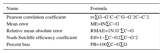
4.2Performance measures based on numerical metricsIn the present study, five numerical metrics were used. These metrics are based on a pair-wise comparison to evaluate the performance of the monthly CHIRPS v.2 product, which estimates the amount of rainfall on each rain gauge listed in Table I as follows: Pearson correlation coefficient (r), mean error (ME), relative mean absolute error (RMAE), Nash-Sutcliffe efficiency coefficient (Eff), and percent bias (PB). These metrics are summarized in Table II.
Pearson coefficient measures the linear relationship strength between estimations and observations, varying from -1 to 1 with a perfect positive correlation being 1. ME and RMAE provide information on the error estimation and the average magnitude of error estimations, respectively. ME can take any negative or positive value [mm.month-1] while RMAE acquires only positive values. Both have a perfect score of 0. Eff quantifies rainfall estimations accuracy in relation to the rainfall observations mean, varying from minus infinity to one with a perfect score equal to 1 (McCuen et al., 2006). PB measures the average tendency of estimated values, which can either be larger or smaller than their observed ones, with an optimal value of 0. RMAE and Eff are non-dimensional while PB has units in percentage (Oreskes et al., 1994; Gleckler et al., 2008). For drought monitoring and hydrological purposes, ME and RMAE values close to 0 and Eff values close to 1 are required along with high values of r in order to minimize both overestimation and underestimation of rainfall amounts (Toté et al., 2015).
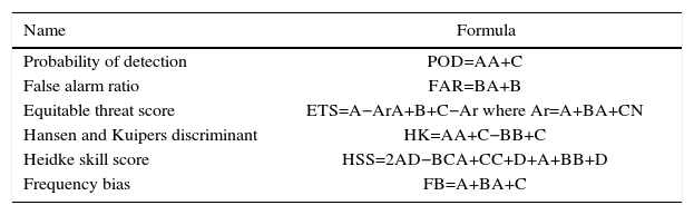
4.3Performance measures based on categorical metricsSix categorical metrics were used in assessing the monthly CHIRPS v.2 product performance for detection of rainfall events on each rain gauge (listed in Table I). These metrics were derived from a contingency table (not shown here) in which letters A, B, C, and D represent, respectively, hits (events forecast to occur which did occur), false alarms (events forecast to occur, but did not occur), missing (events forecast not to occur, but did occur), and correct negatives (event forecast not to occur, and did not occur) with a rainfall threshold of 5 mm (Toté et al., 2015). These metrics are summarized in Table III.
Formulas of performance measures based on categorical metrics.
| Name | Formula |
|---|---|
| Probability of detection | POD=AA+C |
| False alarm ratio | FAR=BA+B |
| Equitable threat score | ETS=A−ArA+B+C−Ar where Ar=A+BA+CN |
| Hansen and Kuipers discriminant | HK=AA+C−BB+C |
| Heidke skill score | HSS=2AD−BCA+CC+D+A+BB+D |
| Frequency bias | FB=A+BA+C |
A: number of hits; B: number of false alarms; C: number of misses; D: number of correct negatives.
The probability of detection (POD) and the false alarm ratio (FAR) indicate the fraction of observed events that were correctly forecasted and the fraction of the predicted events that did not occur, respectively. The equitable threat score (ETS) measures the fraction of observed and/or forecast events that were correctly predicted, adjusted for hits associated with random chance. The Hansen and Kuipers discriminant (HK) shows how well the CHIRPS-based rainfall estimates discriminate between rain and no-rain events. The Heidke Skill Score (HSS) measures the accuracy of estimates accounting for matches due to random chance. The frequency bias (FB) reveals systematic differences between rain events frequency in gauge observations and CHIRPS-based rainfall estimates. POD and FAR vary from 0 to 1; ETS varies from 1/3 to 1; HK and HSS vary from –1 to 1; and FB varies from –∞ to 1. The perfect score for these metrics is 1, except for FAR, which is 0 (Casati et al., 2008; Brill, 2009). For drought monitoring and hydrological purposes, values of FAR and FB close to 0 with ETS and HSS close to 1 are required in order to maximize the detection of rainfall events (Toté et al., 2015).
4.4Identification of spatial patterns based on performance measuresThe results from performance measures were split into categorical and numerical classes; two numerical matrices (154×5 and 154×6 equivalents to stations per metrics) were created subsequently. In order to examine spatial patterns in the performance of CHIRPS-based rainfall estimates, a nonhierarchical cluster analysis, derived from the k-means method, was applied to these numerical matrices (Everitt et al., 2002).
Cluster analysis is a multivariate exploratory data analysis tool used for clustering data into groups using a criterion of similarity (e.g., the Euclidean distance). It has been used as an unsupervised classification technique for verification of precipitation fields derived from numerical models (Marzban and Sandgathe, 2006; Gilleland et al., 2009). In this study, cluster analysis (CA) was used to identify similar stations according to their categorical and numerical performance measures.
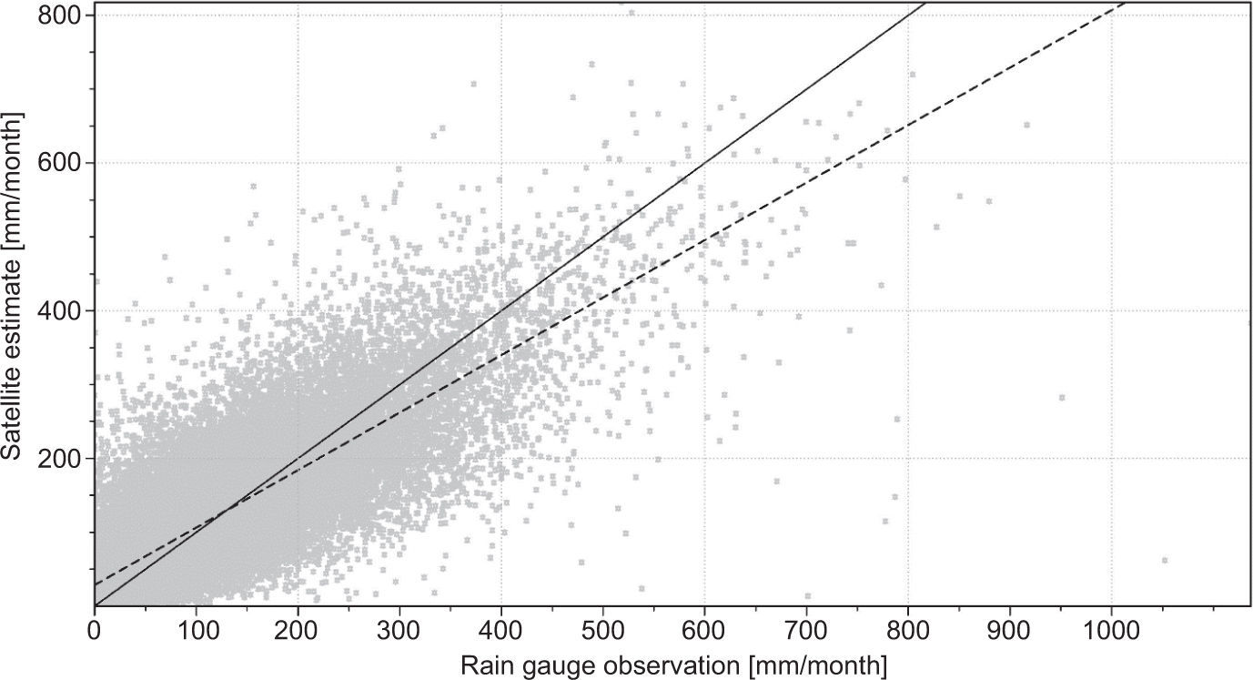
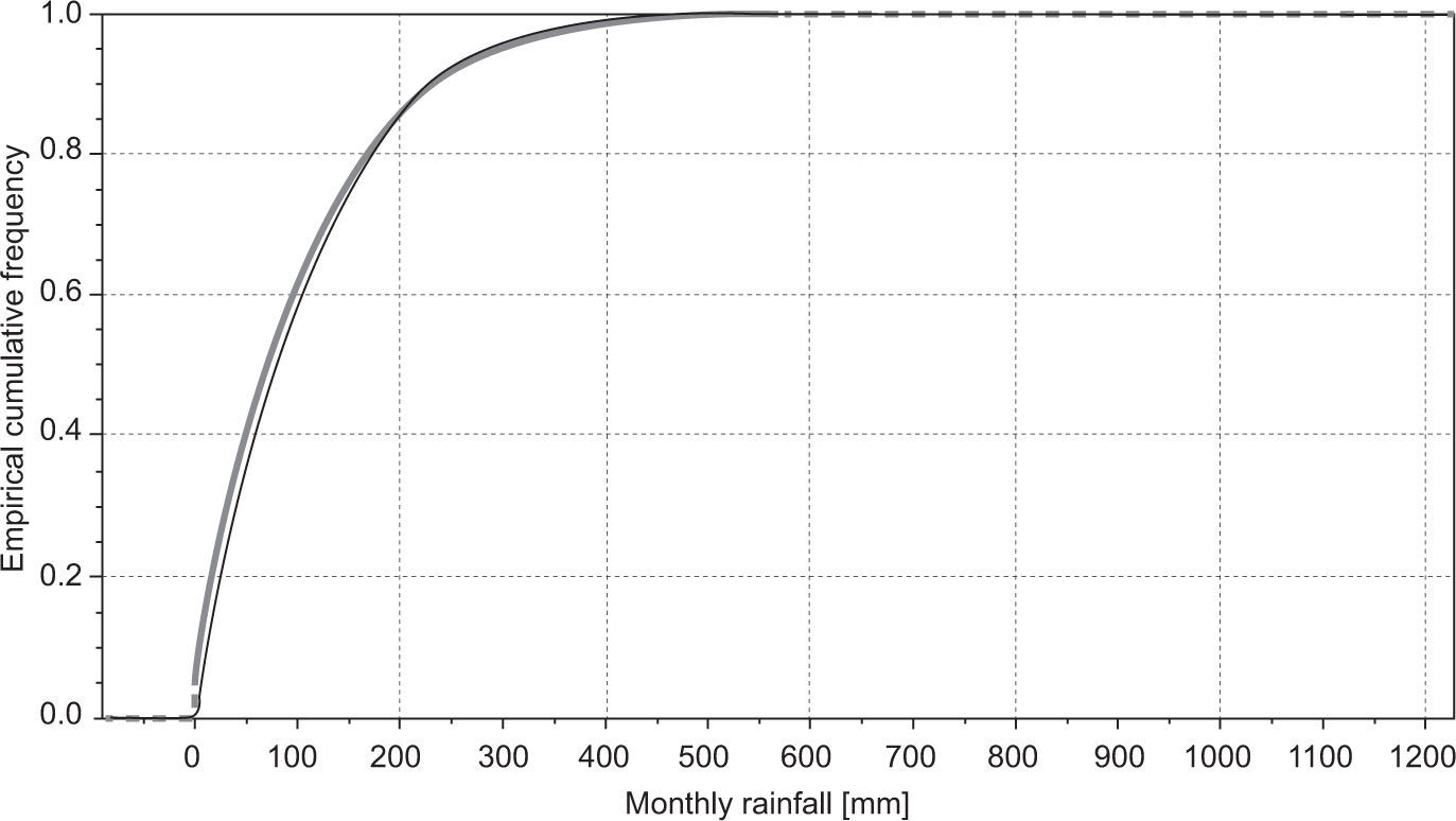
5Results and discussion5.1Overall performance measuresFigure 2 shows rain gauge observations and CHIRPS-based rainfall estimates at monthly scale for the period 1981-2007. Note that the CHIRPS v.2 product exhibits an overestimation of low rainfall values and an underestimation of high values. These features are also evident in their respective cumulative density plots (Fig. 3). In general, Figures 2 and 3 reveal an overestimation in the values of observed rainfall between 0 and about 200 mm/month, whereas for values outside this range the amount of rainfall tends to be underestimated by the CHIRPS v.2 product. One implication of this result is that low rainfall estimates could mask drought conditions (particularly absent rainfall), which is a feature highly unfavorable in drought-prone regions (e.g., the Caroni river hydropower reservoirs system).
. Black line indicates 1:1 correspondence and dashed line gives the linear regression best fit.")

Cumulative density curves for variables shown in Figure 2. The gray and black lines depict ground-based rainfall observations and CHIRPS-based rainfall estimates, respectively.
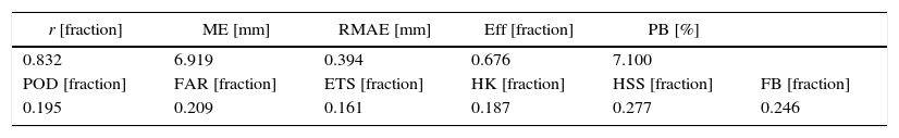
Table IV summarizes performance metrics considering all stations listed in Table I. In general, ME indicates that the CHIRPS v.2 product tends to overestimate rainfall with positive mean errors, which is consistent with the small values of RMAE and PB. On the other hand, the r and Eff metrics are moderately high, suggesting an adequate correspondence between observed and estimated rainfall values. In terms of detection of rainfall events, the CHIRPS v.2 product shows low values of POD, ETS, HK and HSS, and moderately high values of FAR and FB (Table IV), revealing deficient performance. These results warn that the detection of a rainfall event based on the CHIRPS v.2 product is associated to high uncertainty.
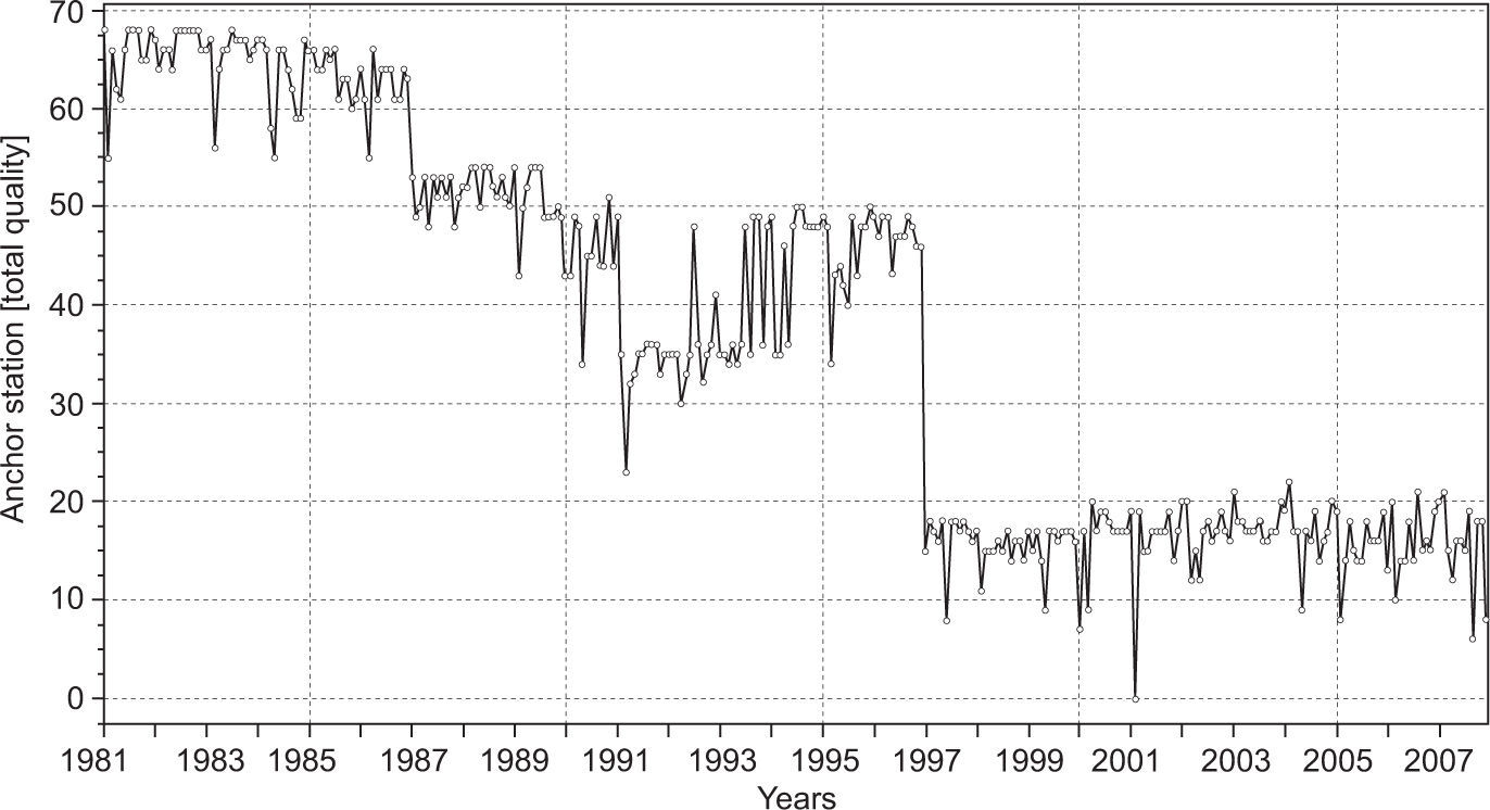
In general, the results from Table IV suggest that CHIRPS-based rainfall estimates might be useful for flood monitoring, but deficient for drought monitoring in the study area. The number of anchor stations used in the creation of CHIRPS in time could help to explain this discrepancy. For example, Figure 4 shows that for the period 1981-1987, between 48 and 68 anchor-stations were used; for the period 1988-1996, between 23 and 54 anchors-stations were used; and for the period 1997-2007, a maximum of 22 anchor-stations were used in the study area. The gradual decrease in number of ground-based observations might have affected the correction stage of the CHIRPS v.2 product, which is reflected as rainfall estimates with low-accuracy (Toté et al., 2015).
5.2Performance measures per rainfall category.")
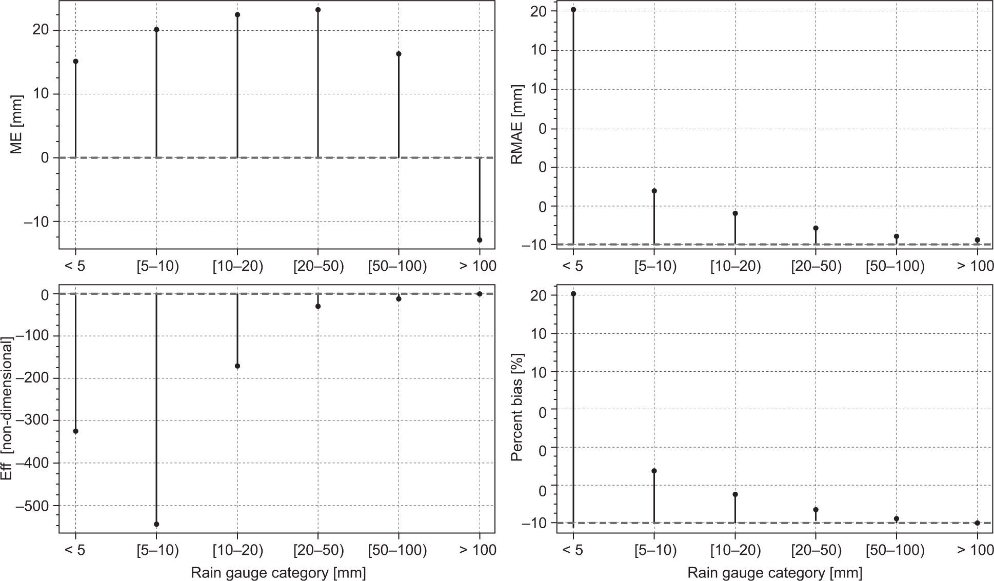
In examining the variability of the measurement performance, according to the observed rainfall amount, all metrics listed in Table IV were calculated for different rainfall categories supported by monthly rainfall observations: < 5 mm, N=5331; [5-10) mm, N=2,096; [10-20) mm, N=3,389; [20-50) mm, N=7,548; [50-100) mm, N=9,002; and > 100 mm, N=16,789 (N indicates the number of pair-wise cases analyzed by category). Figure 5 displays these results. On the whole, higher RMAE, lower Eff, and higher PB can be seen in this figure for low rainfall observations, situation similar and consistent with the inferences made from Figures 2 and 3. Also, it can be noted that rainfall observations less than 100 mm show negative ME values; this means a large overestimation.

The above results support the hypothesis proposed in the previous sections that rainfall estimates from CHIRPS v.2 could be inadequate for drought monitoring applications, although they are suitable for flood monitoring applications given that uncertainty tends to decrease for high rainfall observations.
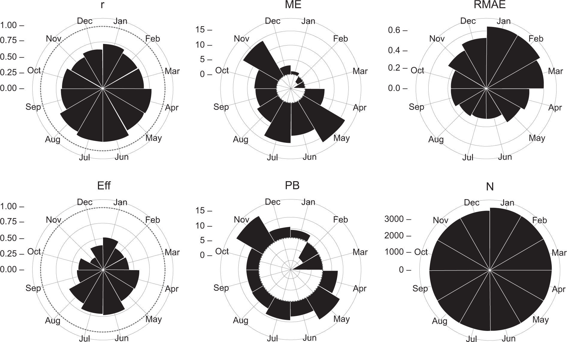
5.3Performance measures in the temporal domainTo zoom in on the performance features of the CHIRPS v.2 rainfall product, this section will focus on the numerical and categorical metrics in the seasonal context. Figure 6 provides the values of the numerical metrics by month for the period 19812007. A difference between the dry and rainy season is evident. During the dry season (October-March), r is lower (mean=0.653), RMAE is worse (mean=0.538), and Eff is lower (mean=0.397). In contrast, for the rainy season (April-September), most metrics perform better. In fact, the correspondence between rainfall estimates and station observations is higher (based on r, mean=0.791), RMAE is lower (mean=0.363), and Eff is higher (mean=0.607).

As Figure 5, but grouped by month. N and r depict the number of pair-wise cases analyzed, as well as the Pearson correlation coefficient by month.
Note that the PB shows an interesting feature in Figure 6. During the rainy season this metric discloses a widespread overestimation with two peaks on May and July (12.2 and 8.9%, respectively). The dry season exhibits an abrupt shift between January and February that the ME metric also depicts. This means that CHIRPS-based rainfall estimates tend to be underestimated throughout January and February, coinciding with the driest period in Venezuela, when high-intensity and spatially isolated convective storms of short duration are frequent, particularly in the plains region (Pulwarty et al., 1992; Sanso and Guenni, 1999).
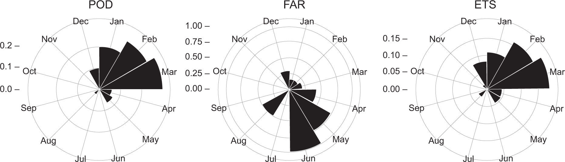
Figure 7 summarizes categorical performance metrics for both seasons. In general, the detection of rainfall events shows its best performance during the dry season (October-March), with higher POD and ETS and lower FAR. Also, note that the CHIRPS v.2 product obtains the highest values of POD and ETS and the lowest ones for FAR from January to March, when rainfall events, linked to the activity of the ITCZ are uncommon in the study area (Williams et al., 2005).

As in Fig. 6, but for POD, FAR, and ETS metrics.
Results from this analysis suggest that the ability to discriminate rainfall events and non-rainfall events from the CHIRPS v.2 product is very deficient; in particular, when the rainy season is taken into account. Therefore, this product cannot be seen as a reliable tool for drought monitoring based on the wet season onset. Toté et al. (2015) suggested that the uncertainty of this product is caused largely by its dependency on 0.25° TRMM training data, which may contribute to its tendency to over-predict in view of the fact that averaging over larger areas increases the frequency of rainfall events. To overcome this limitation, drought indices based on cumulative rainfall in time (such as the Standardized Precipitation Index, which can use a wide range of time scale) could be used (Seiler et al., 2002; Paredes et al., 2015).
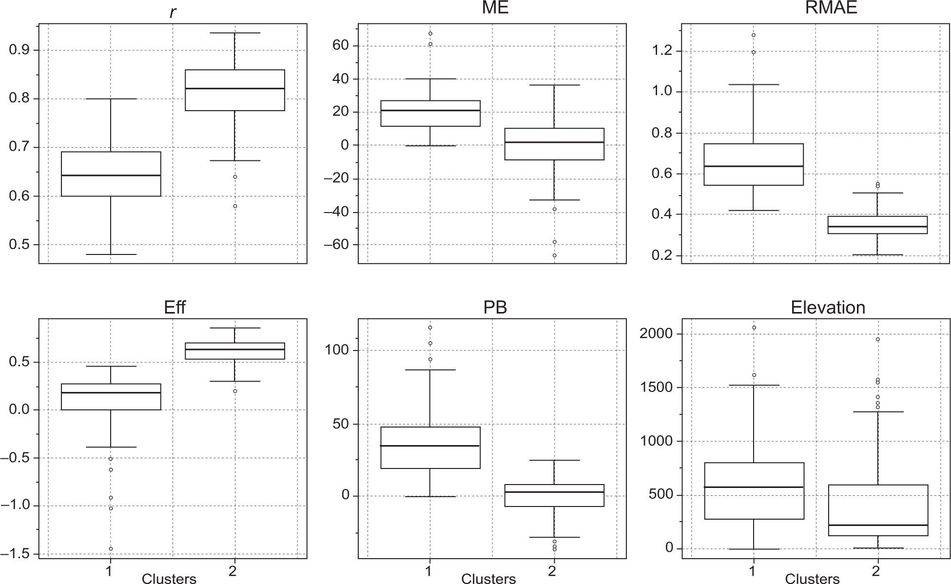
5.4Performance measures in the spatial domainIn order to examine spatial patterns in the performance of CHIRPS-derived rainfall estimates, the performance metrics from each rain gauge shown in Table I were partitioned into numerical and categorical metrics. Next, a cluster analysis was applied to both matrices to identify homogeneous stations according to the similarity of performance metrics. Two clusters were identified for both groups. For comparison purposes, the numerical and categorical performance metrics for each cluster were assessed through boxplots.
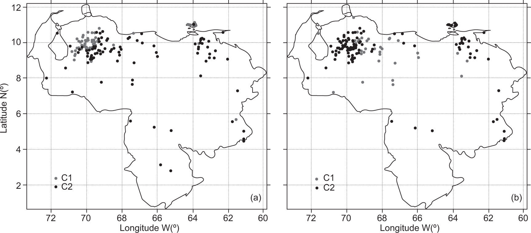
Figure 8 presents a comparison between numerical metrics, while Figure 9a displays the spatial distribution of the clustered stations. For all numerical metrics, the C1 cluster shows the worse performance. Note that the stations that belong to the C1 cluster are mainly concentrated in the northwest region of Venezuela and Margarita Island. Furthermore, most of the stations clustered in C1 are located in the leeward part of the Andes (Figs. 1 and 9a). This feature is interesting because it is well known that these mountains induce prevailing dry climate in several regions of South America (Giovannettone and Barros, 2009). In this latter region, orientation and topographic features facilitate the blocking of the east trade winds and their channeling off this region. Thus, most rainfall events are induced by an isolated convective activity (Insel et al., 2010). At the same time, unlike the rest of the country where a unimodal pattern is dominant, the rainfall regime in this region shows a bimodal pattern (Pulwarty et al., 1992). In contrast, the stations clustered in C2 are largely located in flat open areas where there is a prevalence of convective rainfall driven by the location and activity of the ITCZ and other tropical disturbances (Sanso and Guenni, 2000).
. Eff and r, as non-dimensional fraction; ME and RMAE in mm; PB in percentage; elevation in masl.")
Numerical performance metrics grouped by cluster. Clustered stations are statistically different at the 95% confidence level for r, RMAE, Eff and elevation (based on the Welch two sample test applied to each numerical metric). Eff and r, as non-dimensional fraction; ME and RMAE in mm; PB in percentage; elevation in masl.
 numerical metrics, and (b) categorical metrics. Clustered stations displayed in (a) and (b) correspond to clusters displayed in Figs. 8 and 10, respectively.")
A factor less evident that could influence the numerical performance of the CHIRPS product is the station distances in relation to coastline (not shown in Fig. 8). In fact, the results highlight the importance of this factor in Margarita Island (north of the western coastline; see Fig. 1), where the stations near the coastline show a better numerical performance than those located more inland (statistic evidence at the 95% confidence level).
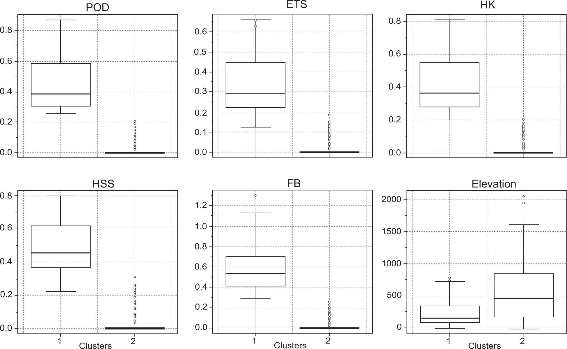
Figure 10 shows a comparison between categorical metrics, while Figure 9b displays the spatial distribution of the clustered stations. For all numerical metrics, the C1 cluster shows the best performance. The contrast found in Fig. 9 indicates that most stations clustered in C2 during the validation procedure based on numerical metrics, show poor performance in the detection of rainfall events (also clustered in C2). These results suggest that the CHIRPS v.2 product tends to show best overall performance in flat open regions. This hypothesis is consistent with the one found by Toté et al. (2015) for Mozambique, which is a tropical country whose topographic features are similar to those of Venezuela. In addition, previous studies have shown that the accuracy of high-resolution satellite rainfall products tends to decrease over complex terrains (Vicente et al., 2002; Dinku et al., 2008, 2011).
. All as none-dimensional fractions, except RMAE in mm and elevation in masl.")
As in Fig. 8, but for categorical performance metrics. Clustered stations are statistically different at the 95% confidence level (based on the Welch two sample test applied to each numerical metric). All as none-dimensional fractions, except RMAE in mm and elevation in masl.
The satellite-based rainfall dataset derived from the CHIRPS v.2 product was analyzed against a rain gauge dataset provided largely by the Instituto Nacional de Meteorología e Hidrología of Venezuela. The CHIRPS v.2 product has a high spatial and temporal resolution which makes it potentially useful for drought and flood monitoring. Rain gauges in Venezuela are sparse, poorly distributed, and often have a high percentage of gaps in their observations. On the other hand, satellite rainfall estimates have random errors and bias due to the indirect relation between observations and precipitation, along with inadequate sampling and algorithm imperfections (Toté et al., 2015). In this study, the analyses were focused on numerical indicators for evaluating the performance of the CHIRPS v.2 product to estimate the amount of rainfall, and categorical indicators to assess its rain-detection capabilities.
Overall, the CHIRPS v.2 product shows an overestimation of lower monthly rainfall values and an underestimation of higher values (≥ 100 mm/month). The coherence between rainfall estimates and station observations is moderately high along the rainy season, but shows a marked underestimation during the driest period, in particular from January to February. Due to its tendency to misclassify rainfall events, especially along the rainy season, the CHIRPS v.2 product has a low skill of rain detection. This high uncertainty in rain detection indicates that it should not be used for drought monitoring in Venezuela; however, this limitation can be partially overcome by using drought indices such as the Standardized Precipitation Index, which is based on cumulative rainfall instead of the presence or non-presence of precipitation.
Estimates of rainfall were also analyzed under a spatial context. Our results indicate that the CHIRPS v.2 product tends to show best performance in flat open regions (e.g., Los Llanos), where the synoptic-scale weather system is mainly dominated by ITCZ activity and local convective systems.
As a whole, the CHIRPS v.2 product may show an acceptable performance when it is used for hydrological applications based on monthly rainfall amounts (e.g., reservoir systems monitoring), but caution must be taken when trying to identify the onset of rainfall for agricultural purposes (e.g., irrigation management in drought-prone regions).
This research was funded by CAPES/CEMADEN/ MTCI Edital Pro-Alertas No. 24/2014 under the projects “Análise e Previsão dos Fenômenos Hidrometeorológicos Intensos do Leste do Nordeste Brasileiro”, and 26001012005P5 PNPD-UFAL/ Meteorology.