Changes in GDP's measurement error volatility and response of the monetary policy rate: Two approaches

Abstract

Using a stylized model in which output is measured with error, we derive the optimal policy response to the demand shock signal and to changes in the measurement error volatility from two different perspectives: the minimization of the expected loss (from which we derive the ‘standard’ policy) and the minimization of the maximum possible loss across all potential scenarios (from which we derive the ‘prudent’ or ‘robust’ policy). We find that (1) the prudent policymaker reacts more aggressively to the shock signal than the standard one and (2) while the standard policymaker always mitigates her reaction if the measurement error volatility rises, the prudent one may even increase her response if her risk aversion is very high. When we incorporate forward-looking expectations, the second result is preserved but, in this case, the prudent policymaker is less aggressive than the standard one in responding to the shock signal.

Resumen

Usando un modelo estilizado en el que el producto se mide con error, determinamos la respuesta de política óptima a la señal del choque de demanda y a los cambios en la volatilidad del error de medición desde dos perspectivas diferentes: la minimización de la pérdida esperada (de la que derivamos la política “estándar”) y la minimización de la pérdida máxima en todos los escenarios posibles (de la que derivamos la política “prudente” o “robusta”). Observamos que: (1) el tomador de decisiones de política prudente reacciona de manera más agresiva a la señal de choque que el decisor estándar y (2) mientras que el decisor estándar siempre atenúa su reacción si aumenta la volatilidad del error de medición, el decisor prudente puede aumentar incluso su respuesta si su aversión al riesgo es muy alta. Cuando incorporamos las expectativas futuras, el segundo resultado se mantiene, pero, en este caso, el decisor prudente es menos agresivo que el estándar en su respuesta a la señal de choque.

1

Introduction

In general, increments in the volatility of an estimated variable could be attributed to an increase in the volatility of the actual variable or to an increase in the volatility of its measurement error.

In practice, increments in the error volatility of estimated macroeconomic variables hinder the process of taking the appropriate economic policy measures. In the decision-making process, the first step is to try to determine what proportion of the observed increase in volatility is the result of measurement error and, once this is established, the second step is to determine what is the optimal policy reaction given these circumstances.

This paper focuses on the analysis of the second step assuming that the increase in volatility corresponds exclusively to measurement error. Specifically, the paper analyzes from two different perspectives how monetary-policy actions should change when there is higher volatility in the measurement error of the aggregate economic activity.

The first perspective corresponds to the standard problem of loss minimization by the monetary policymaker. The second perspective has had good reception recently in economics and corresponds to the concept of “robustness” in which the policymaker seeks to minimize the maximum possible loss across all potential conditional¹ scenarios as a form of prudence to avoid huge losses.

Previous literature has explored the effect of uncertainty on optimal decision making in the framework of optimizing models. Aoki (2003), in a model with nominal price stickiness and asymmetric information, concludes that a central bank that seeks to minimize its expected loss but that faces uncertainty about the actual state of the economy, would exhibit some degree of cautiousness, that is, the central bank would not respond too strongly to noisy indicators of the economy. In the context of a model with symmetric information, Svenson and Woodford (2003) conclude that the optimal response to the imperfect observation of output depends on the noise contained in its indicator.²Orphanides (2003) shows that inefficient policy rules are followed if the noise in signals of economic variables is not taken into account, resulting in excessively activist policy. In that sense, policy reactions should be cautious and less sensitive to unfiltered data.

A general result in this literature is that policymakers should recognize the existence of measurement errors in the information at their disposal, and therefore they should act cautiously in the sense of avoiding overreaction. This result is found assuming that the policymaker knows the distribution function of all possible events and minimizes the expected loss of those events, that is, all the above-mentioned papers study the problem of noisy indicators from what we call the standard perspective.

With regard to the second perspective, attention has being brought to the fact that in most instances policymakers do not know the probabilities of all relevant scenarios and therefore it is not possible to calculate the expected loss of a given policy. One alternative solution for taking policy decisions in this environment is robust control or prudence. This approach looks for the policy that avoids large losses in all possible events, regardless of how likely they are. In the words of Barlevy (2009), “the robust control approach argues for picking the policy… under which the largest possible loss across all potential outcomes is smaller than the largest possible loss under any alternative policy” (p. 40).

This criterion has been considered for the design of optimal policies under uncertainty and it is widely discussed in Hansen and Sargent (2007) and Barlevy (2009). A prudent central bank seeks to minimize the social loss in the worst scenario and though its average performance is, by construction, lower than that of the central bank that minimizes the expected loss, following the prudent policy allows the policymaker to avoid scenarios that have low probability but are very costly. More intuitively, as in an example given by Feldstein (2003), a prudent man is the one who carries an umbrella even when the weather forecast says the probability of rain is low because the small inconvenience of doing so avoids the larger trouble of being caught in a downpour.

In some frameworks, like in Sargent (1999), Giannoni (2002), and Onatski and Stock (2002), the conclusion is that policymakers facing uncertainty should respond more aggressively than policymakers facing no uncertainty. However, aggressiveness is not a general feature of prudence. In other examples, as Barlevy (2009, 2011) show, cautiousness is recommended. The different results under robust controls come from the particular features of the economic environments studied in each case.

In the present paper, we set up a stylized model which incorporates two features: first, the output gap exhibits some degree of persistence; and second, a lag in the effect of monetary policy such that it affects the output gap more rapidly than inflation. The output gap is measured with error (i.e. there is a noisy signal of the demand shock), and therefore monetary policy faces uncertainty.

We derive both the optimal standard policy and the optimal prudent policy responses to the demand shock signal and to an increase in the measurement error volatility. We find that in both cases the central bank reduces (increases) the interest rate when it receives a signal of a negative (positive) demand shock. However, for the same value of the signal, the prudent policymaker reduces (increases) the interest rate more than the standard one.

Furthermore, when there is an increase in the volatility of the measurement error, the standard central bank attenuates its response, that is, when facing a signal of a negative (positive) demand shock but under higher volatility of the measurement error, a standard central bank does not reduce (increase) the interest rate as much. The result is not as straightforward for the case of a prudent central bank. For this type of bank, an increase in the volatility of the measurement error could lead to either an attenuation of its reaction (as in the standard case) or an even stronger response in the interest rate. It depends on which of the following two effects dominate when the volatility increases: the signal's weight in agents’ expectations, or the bank's risk aversion. If the first, then the prudent policymaker attenuates its policy.

In the final part of the paper we extend the model to incorporate forward-looking expectations. The model becomes more complex and for the analysis of prudence we derive conclusions from numerical solutions for a specific set of parameters. In this case we find that the second result is preserved, i.e. while the standard central bank always mitigates its reaction if the measurement error volatility rises, the prudent one may even increase its response if its risk aversion is very high. However, the first result is different; the prudent policymaker is less aggressive than the standard one in responding to the shock signal.

To our knowledge, the closest work to ours is by van der Ploeg (2009). He studies, from a prudent perspective, the optimal response when there is a measurement error of the output gap and there are monetary policy lags and finds that a prudent central bank makes more use of faulty data and hence adopts a more aggressive policy response. van der Ploeg (2009) analyzes the problem using the accelerationist Phillips curve, in which expectations are adaptive. Instead we analyze the problem of measurement errors using rational expectations in two different forms: one, as in the traditional Lucas supply curve, where the relevant expectations are those formed with information up to the previous period (the results in this case are similar to those found by van der Ploeg, 2009) and the other with forward-looking expectations.

In the following section, we describe the model and its equilibria under both criteria. In Section 3, we do the same for the model with forward-looking expectations. Section 4 contains our conclusions.

2

The model and two possible solutions

In a simple model we intend to capture some stylized monetary-policy facts. In particular, it incorporates two features: first, some degree of persistence for the output gap and second, a lag such that monetary policy affects output more rapidly than inflation.

The period loss function for the central bank is

where π is inflation, y is the output gap and λ>0 represents the relative weight given to output stabilization. The Phillips curve (PC) and the IS curve are:

where Et−1 is the expectations operator, conditional on information available at time t−1,³ρ∈(0,1) represents the output's degree of persistence, η∈(0,1), δ and α are positive constants, i is the nominal interest rate and d is the demand shock, which we assume is uncorrelated over time and normally distributed with zero mean and variance σd2 (i.e. dt∼iidN(0,σd2)).⁴ In this setup, changes in the real interest rate have effects on the output gap with a one-period lag and on inflation with a two-period lag.

This economy also has a statistics office whose purpose is to measure the output gap with the highest precision. In any period t, this office releases a provisional estimation of the output gap for the same period (ytˆ) and the final estimation of the same variable for the previous period (yt−1). The former estimation contains a measurement error (i.e. ytˆ≡yt+εt, εt∼iidN(0,σε2)) and the latter estimation contains no error.

The timing is as follows: (1) the statistics office releases ytˆ and yt−1. (2) Private agents form rational expectations. (3) The central bank picks it. (4) Shocks dt and εt are realized but they are unobserved.

Taking into account this timing and the fact that we assume that neither the central bank nor private agents have private information, the information set of the latter when forming expectations in t is

where Θ represents all the constant parameters in the model, including σd2 and σε2. Since the central bank sets the interest rate after observing expectations, its information set in t is

2.1

Solutions

2.1.1

Criterion 1: minimization of the expected loss

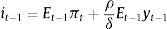
The central bank picks it−1 so as to minimize the expected loss. This is the standard approach to solve the model described above. In this case the uncertainty problem can be reduced to a signal extraction problem. The central bank can construct a signal of the demand shock using the available information in period t−1, dˆt−1≡yˆt−1−ρ⁡yt−2+δ(it−2−Et−2πt−1). Using the IS equation and the definition for yˆt−1:

Since εt−1 is unobserved, it cannot be separated from the signal and therefore dˆt−1 is a noisy signal of the demand shock. Following Harvey and De Rossi (2006, chap. 27), the demand shock forecast can be expressed as:

where γ≡σd2/(σd2+σε2) can be interpreted as a signal-to-noise ratio. The higher the relative amount of noise (σε2/σd2), the lower the weight given to the signal. In the extreme, when the relative amount of noise is infinite, the signal is completely useless and the best forecast for dt−1 becomes its unconditional expected value (zero).

The model is solved by backward induction. The central bank sets it−1 in order to minimize⁵

The solution to this problem yields⁶

where Et−1yt−1=ρ⁡yt−2−δ(it−2−Et−2πt−1)+γ⁡dˆt−1. Since Et−1yt=ρ⁡Et−1yt−1−δ(it−1−Et−1πt) the central bank is setting it−1 in order to set Et−1yt=0 (due to the policy lag, Et−1πt is not relevant as it cannot be affected by it−1).

Using the Phillips curve, we can find the following expression for expectations

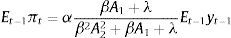
Then, from Eqs. (1) and (2) we obtain

The reduced-form representation of an optimal policy depends, as pointed out by Aoki (2003), on the information structure and the stochastic processes of the economic shocks. From Eq. (3) and the expression for Et−1yt−1 one can see that the optimal policy in our model depends on the lagged nominal interest rate, the lagged inflation expectations, the past output and the shock signal. The fact that a policy rule involves the lagged interest rate may lie on different reasons; for instance, due to the incorporation of interest-rate stabilization as one of the central bank's objectives. In the case of Aoki's (2003) model where inflation and output are subject to measurement errors and shocks are persistent, the central bank needs to use the past interest rate (among other lagged variables) to identify the economic shocks. In our model, by cause of the uncertainty about the exact value of the output gap, the central bank needs to estimate its value, which in turn involves the past output gap (due to output persistence), the lagged real interest rate (due to the monetary policy lag) and the signal of the demand shock.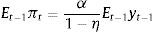

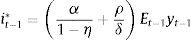
The change of this policy reaction to changes in the demand shock signal is (taking into account that ∂Et−1yt−1/∂dˆt−1=γ)

As it is standard, a higher demand-shock signal increases the policy response of the central bank. This response is mitigated by the coefficient γ which acts as a filter of the noisy signal. As explained above, if the amount of noise is infinite the signal is completely useless, i.e. γ→0. In this case, the monetary policymaker does not react to such signal.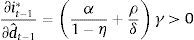

Since γ depends on the measurement error volatility σε2, when such volatility changes the effect on the policy response can be expressed as

This is also a standard result. An increase in the measurement error volatility implies a higher proportion of noise in the signal, and therefore the central bank's optimal response to changes in the signal is reduced.

2.1.2

Criterion 2: robustness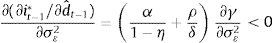

In this scenario we assume that the central bank plays a min–max game against a ‘cruel’ nature. The latter observes what the former does and then acts with the purpose of maximizing the loss. Following van der Ploeg (2009), we construct the stress function which is based on the loss function and the prudence degree of the policymaker:

where θ>0 is inversely related to the central bank's risk aversion and the last term in the equation incorporates the fact that there is a finite level of prudence, and therefore nature cannot impose an infinite cost on the central bank.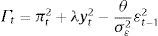

Since the model is solved by backward induction we start at the last stage in which nature sets εt−1 so as to maximize

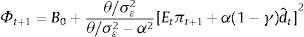
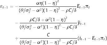
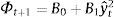
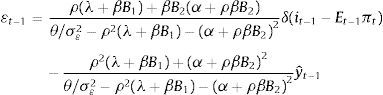
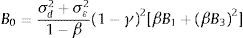
where β∈(0,1) is the discount factor and Φt+1 corresponds to the value function of the problem. It can be verified that such function takes the following form:

where B0 is a constant term. By maximizing (7) we find that nature picks εt−1 following⁷

where yˆt−1=ρyt−2−δ(it−2−Et−2πt−1)+dˆt−1, C≡δρλ(1−η)2+δα2βθ/σε2[ρ/(θ/σε2−α2)]>0.

Taking into account Eq. (8) we proceed to solve the central bank's problem, i.e. to minimize (7) with respect to it−1, which yields⁸

where D1≡(ηρα+δ(θ/σε2−α2))/(δ(θ/σε2−α2))>1 and D2≡((θ/σε2)/(θ/σε2−α2))>1.

Agents expectations are obtained from the Phillips curve and the final expression is equal to that obtained for the standard case (i.e. Eq. (2)). Then the final expression for the monetary instrument is

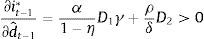
The change of this policy reaction to changes in the demand shock signal is (taking into account that ∂Et−1yt−1/∂dˆt−1=γ)

As in the standard case, a higher demand-shock signal increases the policy response of the central bank. However, since D1>1 and D2>1, the response of the prudent central bank to changes in the signal is greater than that of the standard one (compare (10) with (4)).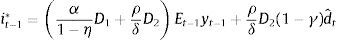

When the measurement error volatility σε2 changes, the effect on the policy response is

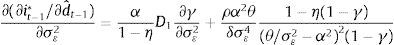
The right-hand side has two opposite effects and, as a result, the total effect can be positive or negative. The first factor corresponds to the impact on the signal's weight in agents’ expectations. When the measurement error volatility increases, the signal has less weight when forming expectations (∂γ/∂σε2<0) and, through this channel, it is less relevant for the central bank. The second factor corresponds to the impact on prudence. Increases in σε2 raise the central bank's relative prudence, as can be seen in its loss function.

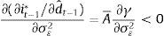
It can be shown that the derivative of the left-hand side with respect to θ is negative. For small-enough values of θ (θ→α2σε2), the prudence factor prevails, and the central bank responds more strongly to the signal when there is a perceived increase in the measurement error volatility (∂(∂it−1∗/∂dˆt−1)/∂σε2>0). On the other hand, when θ is big enough (θ→∞), the factor associated to the signal's relevance prevails. In this case, a prudent central bank attenuates the response to shocks, similar to the standard central bank; however, the former attenuates less⁹ than the latter.

3

Extension: forward-looking expectations

In this section we provide the model's solution when the relevant expectations are forward looking. In this case, the model becomes more complex and for the analysis of robustness we derive conclusions from numerical solutions for a specific set of parameters.

In particular, with respect to the original model (Section 2) we only change the Phillips curve:

where we have assumed that, as in the standard New Keynesian Phillips curve, the coefficient on forward-looking expectations is equal to the discount factor, β. The timing of the model remains the same.

3.1

Solutions

3.1.1

Criterion 1: minimization of the expected loss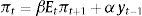

The model is solved by backward induction. The central bank sets it−1 in order to minimize:

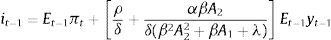
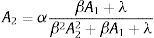
where Vt+1 corresponds to the value function of the problem. Given the monetary policy lag, Lt−1 is irrelevant for the decision about it−1. To obtain a solution for the central bank's problem we postulate the following forms for the value function and expectations:

It should be the case that A1>0 as Vt+1 is the expected discounted value of future losses (all of which must be nonnegative). The optimal interest rate in t−1 is¹⁰

Using the foregoing equation, as well as (PC′) and (13), we can find the following expression for expectations

which is consistent with the postulated form (13) as long as

Then, using the obtained results (Eqs. (14) and (15)) we can verify that

which is consistent with the postulated form (12) as long as A1=αA2.¹¹ From (14), (15) and (16):

where A¯≡A2+(ρ/δ)+((α−A2)/(δβA2))>0 (from Eq. (16), A2<α).

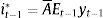
The change of this policy reaction to changes in the demand shock signal is

Since γ depends on the measurement error volatility σε2, when such volatility changes the effect on the policy response can be expressed as

As in the original model: (1) an increment in the value of the demand shock signal increases the policy response of the central bank and such response is mitigated by the coefficient γ; and (2) an increase in the measurement error volatility implies a higher proportion of noise in the signal, and therefore the central bank's optimal response to changes in the signal is mitigated.

3.1.2

Criterion 2: robustness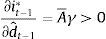

The stress function is equal to that of the original model (Eq. (6)). The model is solved by backward induction. In the last stage nature sets εt−1 so as to maximize

where Φt+1 corresponds to the value function of the problem. To obtain a solution for the central bank's problem we postulate the following forms for the value function and expectations:

Nature picks εt−1 following¹²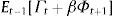

Taking into account the foregoing equation we proceed to solve the central bank's problem, i.e. to minimize (20) with respect to it−1, which yields¹³

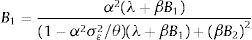
Using equations (PC′), (22), (23) and the fact that yˆt−1=Et−1yt−1+(1−γ)dˆt−1 we can find the following expression for expectations

which is consistent with the postulated form (22) as long as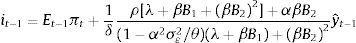

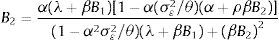
and

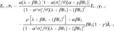
Then, using the obtained results we can verify that

which is consistent with the postulated form (21) as long as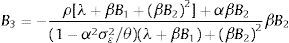

and

From (23), (24) and yˆt−1=Et−1yt−1+(1−γ)dˆt−1:

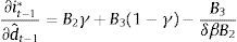
The change of this policy reaction to changes in the demand-shock signal is:

We verify that, for a large set of parameter values,¹⁴ this expression is positive as it was under the criterion of minimization of the expected loss, in Section 3.1.1, and in both cases for the original model in Section 2. However, while in the original model we find that it is always the case that the prudent central bank reacts more aggressively to a higher demand-shock signal, in the present model (with forward-looking expectations) it only happens (for the set of parameters analyzed) when the measurement error volatility is large (and therefore the ratio θ/σε2 is very small). In general, for the present model, the prudent central bank reacts less aggressively to the demand shock signal. The influence of forward-looking expectations on the transmission mechanism reduces the damage that nature can cause and hence, as Barlevy (2009) remarks, the robustness criterion does not necessarily imply that policy should be always more aggressive in the face of uncertainty.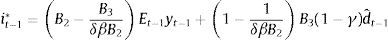

Since γ, B2 and B3 depend on the measurement error volatility σε2, when such volatility changes the effect on the policy response can be expressed as

In this case the value of this derivative may be either positive, as in the case under the criterion of minimization of the expected loss, or negative. Whether it is positive or negative, as in the original model and for the set of parameters analyzed, depends on the value of the ratio θ⁡/σε2. When this ratio is very small, risk aversion prevails in the final effect and a prudent central bank is willing to be more aggressive when it perceives an increase in the measurement error volatility. In contrast, if the ratio θ/σε2 is not small, the dominant effect is that related to the fact that the signal is becoming noisier, and therefore the central bank's optimal response to changes in the signal is reduced. However, such reduction is lower (i.e. when it is negative, the value of (29) is smaller in absolute value) than the one that occurs under the criterion of minimization of the expected loss.

4

Conclusions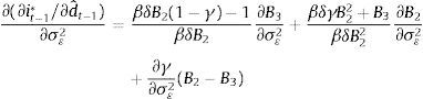

We set up a stylized model which incorporates two features; first, the output gap exhibits some degree of persistence and second, a lag in the effect of monetary policy such that it affects the output gap more rapidly than inflation. The output gap is measured with error and therefore monetary policy faces uncertainty.

We derive the optimal policy response to a noisy signal of the demand shock and to changes in the measurement error volatility from two different perspectives: the minimization of the expected loss (which we refer to as the ‘standard’ perspective) and the minimization of the maximum possible loss across all potential scenarios (which we refer to as the ‘prudent’ perspective).

We find that (1) the prudent policymaker reacts more aggressively to the shock signal than the standard one and (2) while the standard policymaker always mitigates her reaction if the measurement error volatility rises, the prudent one may even increase her response if her risk aversion is very high. The second result is preserved when we incorporate forward-looking expectations but, with regard to the first one, the prudent policymaker is less aggressive than the standard one in responding to the shock signal. The influence of forward-looking expectations on the transmission mechanism reduces the damage that nature can cause and hence, as Barlevy (2009) remarks, the robustness criterion does not necessarily imply that policy should be always more aggressive in the face of uncertainty.

Conflicts of interest

The authors have no conflicts of interest to declare.