Optimal bank credit financing and cost-reducing knowledge for a supplier under different channel structures

Abstract

This study examines a supply chain consisting of a capital-constrained supplier and a retailer. The supplier sells wholesale products to consumers through the retailer and may also sell directly to consumers via an online channel. Given that the supplier’s initial working capital may be insufficient to cover production, investment, or online channel expenses, they have the option to borrow funds from a bank—a practice referred to as bank credit financing (BCF). We develop models with and without direct selling and BCF to analyze the supplier’s optimal decisions regarding cost-reducing investments and the BCF policy. Our findings indicate that, in the absence of direct selling, the supplier’s optimal BCF decision depends on its initial working capital and the investment cost factor. Notably, BCF can enable the supplier to shift from forgoing cost-reducing investments to actively engaging in them when the initial working capital falls within a certain range. Furthermore, under the direct selling model, the supplier’s optimal decision is influenced by a combination of factors, including its initial working capital, investment cost factor, and direct selling cost.

Introduction

Global supply chains have faced unprecedented disruptions in recent years due to macroeconomic volatility, geopolitical tensions, and structural shifts in trade and production networks. Among the most pressing challenges are the financing constraints and rising cost pressures confronting suppliers, which threaten their operational stability and, by extension, the overall resilience of supply chains. The post-pandemic economic landscape has been marked by tightened credit conditions, inflationary pressures, and elevated borrowing costs, making it increasingly difficult for suppliers—particularly small and medium-sized enterprises (SMEs)—to secure affordable financing. Meanwhile, soaring input costs (e.g., raw materials, energy, and labor), coupled with logistical bottlenecks and regulatory compliance burdens, have squeezed profit margins, forcing many suppliers to cut back on critical investments in innovation and capacity expansion. These financial and operational strains have far-reaching implications for supply chain competitiveness. Suppliers struggling with liquidity shortages are more prone to production delays, quality issues, or even insolvency, which can ripple through entire supply networks. Moreover, the consolidation of suppliers due to financial distress reduces market diversity, potentially leading to higher costs and reduced flexibility for downstream buyers. Despite growing recognition of these challenges, there remains a need for deeper analysis on how financing constraints and cost pressures interact to shape suppliers’ optimal decisions, such as direct channel opening strategy, cost-reduction investment strategy, and bank credit financing (BCF) decision.

The rapid development of information technology has increased the popularity of online shopping. According to the “E-Commerce in China” report compiled by the Ministry of Commerce of China, online retail sales reached 15.42 trillion yuan in 2023, marking an 11 % increase. As a result, China has maintained its position as the world’s largest online retail market for the 11th consecutive year. This trend highlights the strong profit potential of China’s online retail sector, which has attracted numerous suppliers to establish online channels in recent years. Consequently, the retail market is no longer solely dominated by traditional retailers. However, it is important to recognize that suppliers’ competitive advantage lies in product design, and engaging directly with customers may pose a disadvantage compared to traditional retailers.

Once an online retail channel is established, the supplier’s responsibilities extend beyond product design and production to include the management of online retail activities. This expansion can place a significant strain on the supplier’s financial resources, particularly for those facing capital constraints. During peak sales seasons, the supplier must not only fulfill orders from downstream retailers but also ensure sufficient stock for their direct online sales channels. This dual demand can considerably increase production pressure, necessitating additional funding to support operations. In such cases, suppliers may resort to BCF, a traditional external funding source, to address capital shortfalls. According to the China Daily website, China has implemented an action plan to strengthen financing credit service platforms and facilitate access to capital for SMEs. When these SMEs encounter financial difficulties that hinder their production and sales activities, BCF can provide a solution.

Recently, an increasing number of banks have been offering financing services to manufacturers with favorable credit conditions. However, the supplier’s ability to repay the loan remains a key concern for these banks. Previous studies have shown that demand risk can affect the supplier’s sales and profits (Ji et al., 2017; Li et al., 2016), which in turn influences their ability to repay debt—a factor frequently addressed in the literature on operations-financing interfaces (Zhao et al., 2021a, 2021b). Additionally, the interest rate set by the bank plays a critical role in the debt-repayment capacity of a capital-constrained supplier, often regarded as an exogenous credit risk in supply chain transactions. In practice, the bank typically determines the interest rate based on the borrower’s credit rating. Generally, firms with higher credit ratings can secure lower interest rates, thus benefiting from a reduced cost of capital. In this study, we treat the interest rate as a decision variable for the bank.

Additionally, with the advancement of technology and the intensifying market competition, the need for continual updates to production processes has become more critical than ever. For many operations and technical managers, a key concern is how to achieve cost advantages to remain competitive in the market. Investments in production processes are often considered a means to reduce production costs and gain a competitive edge (Feng & Gu, 2018; Lugovoi et al., 2022). Typically, process investments encompass expenditures on professional technologies, advanced equipment, and human resources, all aimed at cost reduction and efficiency improvement, thereby significantly influencing the competitiveness of firms (Ge et al., 2014). In practice, many companies have adopted investment strategies to lower production costs. For example, Xiaomi has maintained a low-cost business model for its high-performance smartphones by developing proprietary chip processors, which help reduce production costs. Similarly, Apple and Huawei have invested in the development of their own CPUs to minimize the costs of new product lines.

Given the varying levels of working capital available to suppliers and the complexity of the supply chain environments in which they operate, investment methods and objectives differ. After borrowing funds from a bank, how does the supplier allocate the loan? Is it directed toward enhancing cost reduction or expanding online channels? Furthermore, does the supplier’s initial working capital influence its bank financing decisions and the intended purposes for borrowing? This study explores the following research questions:

• (1) How should suppliers with different levels of initial working capital make optimal bank financing decisions under both the “No Direct Selling” and “Direct Selling” settings? Specifically, should the supplier borrow from the bank, and if so, should the loan be used for cost-reduction investments or for expanding online channels?

• (2) What is the impact of investment costs and direct selling costs on the supplier’s optimal decision-making?

• (3) How are the bank’s optimal interest rates influenced by investment costs and direct selling costs?

To address these issues, we consider a supply chain consisting of a capital-constrained supplier and a retailer. The supplier sells wholesale products to consumers through the retailer and may also sell directly to consumers via an online channel. Given that the supplier’s initial working capital may not be sufficient to meet the needs of production, investment, or online operations, the supplier has the option to borrow funds from a bank, which we refer to as “Bank Credit Financing” (BCF). In our study, we develop models with and without direct selling to examine the supplier’s optimal decisions regarding cost-reduction investments and BCF policies under different initial working capital scenarios. We find that, under the no direct selling model, the supplier’s optimal BCF decision is influenced by both the initial working capital level and the investment cost factor. Notably, BCF can enable the supplier to shift from forgoing cost-reduction investments to engaging in such investments when the initial working capital falls within a certain threshold. Additionally, under the direct selling model, the supplier’s optimal decision is affected by a combination of initial working capital, investment cost factors, and direct selling cost.

The remainder of this paper is structured as follows. Section 2 reviews the relevant literature. Section 3 introduces the model setup, including the notation and assumptions. Section 4 examines the supplier’s optimal financing and investment strategies under both the “no direct selling” and direct selling models. Section 5 analyzes the equilibrium outcomes to gain further insights. Section 6 examines how shifts in working capital influence the optimal BCF strategies through empirical investigation. Finally, Section 7 concludes the paper and discusses potential directions for future research. All proofs are presented in the Appendix.

Literature review

This study is closely related to two streams of literature: (i) investment in process improvement for cost reduction and (ii) BCF for firms with capital constraints. We review each stream and highlight our study’s main contribution.

Numerous studies have explored investment in process improvement across various domains. In the field of supply chain and operations management, the issue of process investment has been examined from several perspectives, including investment efficiency (Li & Rajagopalan, 2008), investment decisions under different channel structures (Gupta & Loulou, 1998), and investment decisions in a multi-cycle game context (Bernstein & Kök, 2009). Generally, the focus of this body of literature has been on supply chain coordination. Some scholars have investigated cooperative efforts for cost reduction (Cho & Gerchak, 2005; Chao et al., 2009; Iida, 2012). Many studies have also incorporated competition among supply chain members and analyzed coordination contracts. For example, Dobson and Chakraborty (2020) argue that competition can provide organizational advantages, thereby driving investments in process innovation aimed at cost reduction. Arya et al., 2015 show that simple cost-based contracts, when coupled with the presence of an intermediary, can lead to integrated outcomes, thus reducing production costs. Ha et al. (2017) explored information sharing in competing supply chains in the context of production cost reduction and found that cost-efficient manufacturers benefit from information sharing, while inefficient ones may suffer as it enables wholesale prices to respond to demand signals. In addition, some studies examine spillover effects in competitive environments and optimal process investment strategies (Capuano & Grassi, 2019; Hinloopen & Vandekerckhove, 2009; López & Vives, 2019; Veldman & Gaalman, 2015). More recently, Niu and Shen (2022) examined investment strategies for competitive manufacturers with different absorptive capacities in the context of knowledge spillovers, incorporating innovation uncertainty. Xu and Sun (2019) investigated how manufacturers’ cost reduction and pricing decisions are influenced by strategic customer behavior and found that both cost reduction and initial production costs affect the first-period price under dynamic pricing and price commitment strategies.

The second stream of literature focuses on credit financing for firms facing capital constraints. Bank credit is a traditional external source of funding for firms with capital shortages. Regarding retailer bank financing, Dada & Hu, 2008 suggest that if borrowing costs are not excessively high, a capital-constrained newsvendor will borrow funds, and the lender’s interest rate will decrease as the newsvendor’s equity increases. Kouvelis and Zhao (2011) examined a scenario where a retailer borrows funds from a bank to place orders, with the bank offering loans at an appropriate interest rate based on associated risks and noted that failure to repay the loan can lead to costly bankruptcy. Zhang et al. (2016) explored the impact of loss aversion on the ordering policies of capital-constrained retailers and found that loss aversion can shift the retailer from a capital-constrained to a capital-sufficient position. Some studies have incorporated trade credit financing and compared it with BCF to determine the optimal financing strategy for capital-constrained retailers (Chod, 2017; Hua et al., 2019; Jing et al., 2012; Kouvelis & Zhao, 2012). Shi et al. (2020) examined the effect of bankruptcy costs on a capital-constrained retailer's decision to choose between bank credit financing and trade credit financing. Cheng et al., 2021 analyzed the impacts of preferential credit policies on capital-constrained retailers and found that financing from a risk-seeking bank or the manufacturer can improve the retailer’s optimal order quantity in a coordinated supply chain. Xie et al. (2022) found that dual-channel financing increases the retailer’s order quantity, creating additional value for all participants. Jiang et al. (2022) concluded that a retailer in a supply chain with a well-funded supplier and a small, capital-constrained retailer always benefits from BCF. While these studies focus on credit financing strategies for retailers, the present study investigates the credit financing decisions of capital-constrained suppliers, as well as the cost-reduction investment strategies they adopt.

Specifically, we consider a supplier with an initial amount of working capital and explore how suppliers can make optimal BCF and cost-reduction investment decisions at different levels of initial working capital, with and without direct selling. We demonstrate that the supplier will borrow from the bank if its initial working capital is insufficient, and the loan will be used for production; whether the loan is used for cost reduction depends on the investment factor. Once the supplier establishes an online channel to sell directly to consumers, the optimal BCF decision depends not only on initial working capital and the investment factor but also on direct selling cost. The present study aims to explore the interaction between the investment factor and direct selling cost in determining the supplier’s optimal BCF and cost-reduction strategies under different levels of initial working capital.

Model setup

We consider a traditional retail channel in which a supplier (denoted as S) sells products to the market through a retailer (denoted as R). Besides this retail channel, the supplier may also sell to the consumer directly by operating its direct selling. A supplier focuses on production and its sales process is less efficient than that of a retailer because the retailer has extensive experience in dealing with consumers. Specifically, suppliers’ grasp of market information and information accuracy is not as strong as that of retailers; in other words, compared with retailers, suppliers’ sales efficiency is lower, and they incur a certain sales cost when selling products directly to consumers through online channels. In this study, we normalize the retailer’s unit selling cost to zero and let cs denote the supplier’s unit cost of selling directly to consumers (Arya et al., 2007).¹

In addition, the supplier can engage in cost-reduction investment to gain a cost advantage in the fierce market. Assuming that the production cost can be improved from the initial cost c to c−e after the supplier invests an effort level e. Correspondingly, the effort cost the supplier must bear is k+12ϕe2, where ϕ>0 is the variable cost of the investment, representing investment efficiency.² A higher ϕ indicates lower investment efficiency, as it reflects greater costs required to achieve a specific level of cost reduction. In practice, k captures the factors influencing the cost of process improvement, including the supplier’s production technology and R&D capability. It should be noted that decisions regarding the process improvement level e precede pricing decisions, as component wholesale prices are heavily influenced by cost reduction targets, requiring longer-term planning (Jin et al., 2019). For a capital-constrained supplier, we consider the BCF to fund the supplier’s cost reduction and production.

This study aims to address the following research questions. When should the supplier operate direct sales and how should the dual-channel be managed? What are the optimal cost-reduction strategies for suppliers under different channel structures; should they borrow from the bank? What is the interaction between direct selling and cost reduction, that is, are they strategically complementary or substituted?

Consumer demand for the products is represented by an inverse demand function p=a−bQ, where b represents strictly positive constants and Q=qR+qS is the total quantity consisting the retail quantity qR ordered by the retailer plus the direct sales quantity qS determined by the supplier when it operates direct selling (if the supplier does not operate direct selling, Q=qR). a is the base demand that is known to both firms. To avoid triviality, we assume that the base demand value a is sufficiently large to ensure a non-negative order quantity.

The sequence of events is as follows. First, the supplier decides whether to operate a direct selling channel. Second, the supplier decides whether to engage in cost reduction; if so, selects the BCF to fund cost reduction or invest only by itself. Third, the bank sets an interest rate rB. Fourth, the supplier sets an effort level e after receiving funding from the bank. After the demand is realized, we assume that both the supplier and the retailer can capture the demand information, the supplier charges a wholesale price w for each unit of product from the retailer, then, the retailer chooses its profit-maximizing retail output qR. Finally, the supplier determines the number of units qS of the homogeneous product it will sell to consumers via the direct selling channel. Backward induction is employed to get the equilibrium in each scenario.

The model

In this section, we consider a capital-constrained supplier borrowing from a monopoly bank to finance its production and cost-reduction investment. Assuming that the supplier has an initial working capital y, it would not engage in cost reduction with a minimal initial working capital (y≤k). After borrowing from the bank, the supplier then decides whether to engage in cost reduction. If the initial working capital is higher than the fixed cost of cost-reduction (y>k), the supplier needs to decide whether to engage in cost reduction; if so, whether using the initial working capital or borrowing from the bank?

Model without direct selling or BCF

First, we consider a no-direct-selling setting in which the supplier only sells products to consumers through the retailer. In this setting, the production quantity Q=qR.

Now, we examine optimal cost reduction without BCF in the case where y>k. First, we assume that the supplier will not engage in cost reduction when its initial working capital cannot meet optimal production. In other words, the supplier’s working capital is prioritized for production. If the supplier does not engage in cost reduction, its profit is affected by the initial working capital. If it engages in cost reduction, its profit is affected by not only the initial working capital but also the cost factor of cost reduction ϕ and k. We assume this in Lemma 1.

Lemma 1. The supplier’s profits without BCF under different initial working capital levels are as follows:

When y<(a−c)c4b, the supplier would not engage in cost reduction and obtain π⌣SNN=(a−c)cy−2by2c2 the profit increases as the initial working capital increases. When y≥(a−c)c4b, the supplier achieves the optimal production and obtains its maximum expected profit π^SNN=(a−c)28b.

When y

To avoid triviality, we assume that the supplier would not engage in cost reduction when it cannot achieve the optimal effort level. From Lemme 1, we can see that under the no-direct-selling setting, the supplier engages in cost reduction without BCF only when k

Model without direct selling under BCF

In this setting, the production quantity Q=qR. Then, we investigate the optimal cost reduction with BCF. If the borrowing is only used to expand production, the loan size is LNN=cqR−y. If the purpose of the supplier’s borrowing from the bank is both the expansion of production quantity and higher effort level, the loan size is LNC=(c−e)qR+k+12ϕe2−y. Establishing the decision model of a no-cost-reduction setting and a cost-reduction setting, the equilibriums of these two cases are denoted as “NN”and “NC,”respectively.

Case NN

In this setting, the retailer chooses its order quantity qR to maximize its monopoly profit from retail sales, taking the unit wholesale price w as given. The retailer’s problem is:

Performing the optimization in Eq. (4.1) provides qR(w), the retailer’s order quantity in the no-direct-selling setting given unit wholesale price w:

Assuming that the order quantity decision made after the demand is realized, there is no market risk undertaken by the bank or the supplier. Given an optimal interest rate r, and the retailer’s anticipated response to the wholesale price it sets, the supplier chooses w to maximize its profit,

Substituting LNN and qR(w) into Eq. (4.3) yields the supplier’s profit-maximization wholesale price as a function of the bank’s interest rate r,

Substituting w(r) into Eq. (4.2) yields qRN(r).The monopolistic bank determines an interest rate r to maximize its expected profit by lending to the supplier.

Performing the optimization in Eq. (4.5) yields the bank’s optimal interest rate rNN under a no-cost-reduction setting. The equilibrium in a no-cost-reduction setting is:

rNN=−4by+c(a−c)2c2, wNN=3a+c4−byc, qRNN=c(a−c)+4by8bc,

πSNN=c2(a−c)2+8c(3a+c)by−48b2y232bc2, πRNN=[c(a−c)+4by]264bc2πBNN=(a−c)c8b−y2

To ensure rNN>0, we have y0. Compared the supplier’s profit with and without BCF, πSNN−π⌣SNN=(a−c)2c2−8(a−5c)cby+16b2y232bc2>0.

Thus, the supplier would borrow from the bank to expand its production only when its initial working capital is below c(a−c)4b. The supplier’s expected profit without cost reduction can be written as

the bank’s expected profit without cost reduction can be written as

Case NC

When the supplier engages in cost reduction by borrowing from the bank, substituting LNC and qR(w) into Eq. (4.3) yields the supplier’s profit-maximization wholesale price as a function of its effort level e:

The supplier adjusts the wholesale price according to the effort level of cost reduction, a higher effort level leads to a lower production cost and, subsequently, a lower wholesale price. Substituting wNC(e) from Eq. (4.6) into (4.3) yields the supplier’s expected profit-maximization effort level eNC(r),

Substituting eNC(r) into Eqs. (4.6) and (4.2) yields qRNC(r), where qRNC(r)=[a−c(1+r)]ϕ−1−r+4bϕ. Then, the monopolistic bank determines an interest rate r to maximize its expected profits by lending to the supplier,

The profit function of the bank guides in the first order of r is as follows:

Let M1=(a−4cbϕ)ϕ2(k−y)+ϕc2,M2=33(−1+4bϕ), where y

Solving this equation obtains rC=(1−5N2+N4)(−1+4bϕ)1+N2+N4, where N=M1−M2+M12+M223 .

Substituting rC into Eq. (4.7) yields the optimal effort level in BCF without direct selling eNC, where eNC=c+3N(1+N2+N4)N6−1c2+2(k−y)ϕ. To ensure the existence, uniqueness, and stability of effort-level equilibria, we assume that the cost of effort is large enough. This assumption is not restrictive for most industrial situations (Gupta & Loulou, 1998; Gupta, 2008). Then, we have M1〈0,M2〉0,N<−1. To ensure that the interest is positive, we have 1−5N2+N4>0, which yields N<−5+212. There exists ϕ0N>a4cb, when ϕ>ϕ0N, N<−5+212. In this case, the supplier sets an effort level less than c, and the equilibrium in a cost-reduction setting is as follows:

rNC=(1−5N2+N4)(−1+4bϕ)1+N2+N4, eNC=c+3N(1+N2+N4)N6−1c2+2(k−y)ϕ,

wNC=a2−3N[3N2+2bϕ(1−5N2+N4)]N6−1c2+2(k−y)ϕ,

qRNC=ϕe, πRNC=bϕ2e2, πSNC=3N2(−1+4bϕ)ϕ(1+N2+N4)e2−(1+r)(k−y)

Model with direct selling but no BCF

In this setting, the supplier operates the direct channel to sell products to consumers directly, and the production quantity is Q=qR+qS. If the supplier does not engage in cost reduction, its profit is affected by the initial working capital and the direct selling cost. If it engages in cost reduction, its profit is affected by not only the initial working capital and direct selling cost but also the cost factor of cost reduction. We assume this in Lemma 2.

Lemma 2. The supplier’s optimal profits under different levels of initial working capital without BCF are as follows:

When c(3a+c−26ac−2c2)12b

When y

Assuming that the supplier would not engage in cost reduction when it cannot achieve the optimal effort level, the supplier would engage in cost reduction based on its initial working capital if y≥y0 and k<(a−c−cs)24b(−1+2bϕ); otherwise, it would not engage in cost reduction. Detailed proof of Lemma 2 is shown in the Appendix.

Model with direct selling and BCF

Now, we investigate the optimal cost reduction with BCF. In this setting, the supplier not only operates the direct channel to sell products to consumers directly but also borrows from the bank. The production quantity is Q=qR+qS. If the borrowing is only used to expand the production, the loan size is LDN=c(qR+qS)−y. If the purpose of the supplier’s borrowing from the bank is both the expansion of production quantity and higher effort level, the loan size is LDC=(c−e)(qR+qS)+k+12ϕe2−y. Establishing the decision model of a no-cost-reduction setting and a cost-reduction setting, the equilibriums of these two cases are denoted as “DN” and “DC,”respectively.

Case DN

Given a retail channel quantity qR ordered by the retailer, the supplier chooses its direct selling quantity qS as follows:

The supplier’s revenue is (p−cs)qS+wqR; the first term is the revenue from direct selling, the second term is the payment from the retailer in the retail channel after products are produced. At the end of the period, the supplier’s revenue is used to repay its debt L(1+r). Substituting LDN into Equation (4.8) and performing the optimization yields qSDN(qR),

Anticipating the supplier’s response in direct sales, the retailer determines qR to:

Substituting qSDN(qR) from Eq. (4.9) into Eq. (4.10) and performing the maximization in Eq. (4.10) yields qRDN(w), the retailer’s profit-maximizing order quantity as a function of the supplier’s wholesale price:

Given an optimal interest rate r, and the retailer’s anticipated response to the wholesale price it sets, the supplier chooses w to maximize its profit. Substituting LDN and qRDN(w) into Equation (4.8) yields the supplier’s profit-maximization wholesale price as a function of the bank’s interest rate r:

wDN(r)=3a−cs+3c(1+r)6 (4.12)

Substituting wDN(r) into Eqs. (4.11) and (4.9) yields qRDN(r) and qSDN(r); the monopolistic bank determines an interest r to maximize its expected profit by lending to the supplier:

Performing optimization in Eq. (4.13) yields the bank’s optimal interest rate rDN. The equilibrium in a no-cost-reduction setting is:

rDN=c[3(a−c)−cs]−6by6c2, wDN=c(3a+c−cs)−2by4c, qSDN=2by+c(a−c−3cs)4bc, qRDN=2cs3b, πSDN=c2[9(a−c)2−30(a−c)cs+73cs2]+12c(9a+3c−7cs)by−108b2y2144bc2, πRDN=2cs29b.

To ensure rDN>0, we have y

Therefore, the supplier would borrow from the bank to expand its production when its initial working capital is below c[3(a−c)−cs]6b.

The supplier’s profit without cost reduction can be written as follows:

the bank’s profit without cost reduction can be written as

Case DC

When the supplier engages in cost reduction by borrowing from the bank, substituting LDC into Equation (4.8) yields qSDC(qR); substituting qSDC(qR) into Eq. (4.10) yields qRDC(w); substituting qRDC(w) and qSDC(w) into Equation (4.8) yields the supplier’s profit-maximization wholesale price as a function of its effort level e; and substituting wDC(e) into Equation (4.8) yields the supplier’s expected profit-maximization effort level eDC(r):

Then, we can obtain qSDC(r)=3[a−(1+r)c]bϕ+(1+r−5bϕ)cs3b(−1−r+2bϕ), and qRDC=2cs3b. The monopolistic bank also determines an interest rate r to maximize its profits by lending to the supplier:

When cs>0, the equilibrium in this case can be written as follows:

eDC(r)=a−(1+r)c−cs(−1−r+2bϕ), wDC(r)=[a+c(1+r)]bϕ−a(1+r)−1−r+2bϕ+(2(1+r)−bϕ)cs3(−1−r+2bϕ),

qSDC(r)=[a−c(1+r)]ϕ−1−r+2bϕ+cs(1+r−5bϕ)3b(−1−r+2bϕ),

πSDC(r)=−(k−y)(1+r)+[a−c(1+r)]2ϕ2(−1−r+2bϕ)+(−2−2r+7bϕ)cs2−6[a−c(1+r)]bϕcs6b(−1−r+2bϕ)

πBDC(r)=r{k−y−[a−c(1+r)−cs]2ϕ2(−1−r+2bϕ)2−(a−2cbϕ−cs)[(3a−3c(1+r)−cs)bϕ−cs(1+r)]3b(−1−r+2bϕ)2}

Results analysis

This section analyzes the model’s equilibrium outcomes under various scenarios, examines the supplier’s optimal BCF policy and cost-reduction investment strategy, and explores the impact of direct selling cost on the bank’s optimal interest rate.

The optimal decisions of the supplier without direct selling

We begin by analyzing the supplier’s optimal BCF and cost-reduction decisions without direct selling. The supplier would borrow from the bank to expand its production when its initial working capital is too low (i.e., 0ϕ0N. Due to the complexity of expressions, we use numerical experiments to investigate the impact of ϕ on the bank’s interest rate and the supplier’s effort level of cost reduction, as well as the supplier’s profit changes with the value of ϕ and k. Let a=24,b=1,c=2,y=10,k=1.Figs. 1 and 2 show the impact of ϕ on the bank’s interest rate and the supplier’s effort level.

Fig. 1.

The trend of the bank’s interest rate with ϕ under Case NC.

Fig. 2.

The trend of the supplier’s effort level with ϕ under Case NC.

According to Figs. 1 and 2, ∂rNC∂ϕ>0, ∂eNC∂ϕ<0; as ϕ increases, the supplier interest rate increases, and the supplier reduces its effort level. Then, let a=24,b=1,c=2,ϕ=8,y=10. Fig. 3 shows the supplier’s profit with cost reduction and no cost reduction under BCF. The supplier would engage in cost reduction when the fixed cost is below the threshold k˜. According to Fig. 4, as ϕ increases, k˜ decreases. k˜

Fig. 3.

The trend of the supplier’s profit with k under Cases NN and NC.

Fig. 4.

The optimal decision of the supplier under different k and ϕ values.

When the supplier can achieve the optimal production using its initial working capital (i.e., y≥c(a−c)4b), there is no need to borrow from the bank for production. We investigate whether the supplier would borrow for cost reduction. Consistent with the previous section, mark the suppliers’ profit with cost reduction under BCF as πSNC (see Section 4.2.2 for the expression), engage or forgo cost reduction before BCF as π^SNCand π^SNN(the expressions are shown in Lemma 1). Let a=24,b=1,c=2,ϕ=6,y=12.Fig. 5 shows the trend of the supplier’s profit in different settings. If ϕ is relatively low and the fixed cost is below k0, we have π^SNC>π^SNN>πSNC; that is, the supplier engages in cost reduction using its initial working capital only, and is reluctant to borrow from the bank. If the fixed cost exceeds k0 but is below k1, we have πSNC>π^SNC>π^SNN; the supplier still engages in cost reduction using its initial working capital; however, it would strengthen its effort level by borrowing from the bank. When k1π^SNN>π^SNC; the supplier would not engage in cost reduction using its initial working capital, but it would borrow from the bank. When k2Fig. 6 shows that the supplier will borrow from the bank when the fixed cost of the investment is below k2, and forgo the cost reduction once k>k2.

Fig. 5.

The trend of the supplier’s profit under different Cases (ϕ=6).

Fig. 6.

The trend of the supplier’s profit under different Cases (ϕ=10).

In summary, the optimal decision of the supplier with different levels of initial working capital is summarized as Theorem 1.

Theorem 1. The optimal decisions of the supplier with different levels of initial working capital y in the no direct selling setting are as follows:

If 0

If y≥c(a−c)4b, the supplier can meet the optimal production by itself, the cost-reduction decision using its initial working capital or borrowing from the bank is determined by the fixed cost k and the marginal cost ϕ of the investment for cost reduction:

• a) When ϕ<ϕ0N,kπ^SNN>πSNC.

• b) When k0π^SNC>π^SNN, and the supplier would borrow from the bank to strengthen its effort level.

• c) When k1π^SNN>π^SNC.

• d) When k>k2, the supplier would always abandon cost reduction.

Theorem 1 provides a comprehensive framework for understanding how suppliers with varying levels of initial working capital should approach cost reduction and BCF decisions within a single-channel structure. The theorem highlights the critical role of the supplier’s financial position in determining whether to invest in cost-reduction efforts and whether to seek external financing to support these efforts. This analysis can be expanded to explore the broader implications of financial constraints, cost structures, and market conditions on supplier decision-making, as well as the strategic interplay between internal resources and external financing. The first part of the theorem emphasizes that when a supplier’s initial working capital is insufficient, it may forgo cost-reduction initiatives altogether. In such cases, even if the supplier secures a bank loan, the funds are primarily allocated to expanding production capacity rather than improving cost efficiency. This behavior stems from the supplier’s immediate need to meet production demands and maintain operational viability. The production quantity in this scenario satisfies cqR≤y, meaning the supplier’s working capital is only sufficient to cover basic production costs, leaving no room for additional investments in cost reduction. However, once the supplier achieves optimal production levels using its own resources, the cost-reduction decision to use its initial working capital or borrow from the bank is determined by the cost-reduction factor: If the fixed cost k and the marginal cost ϕ of cost reduction are relatively low, the supplier may choose to fund these cost-reduction efforts internally without resorting to external borrowing. This decision reflects a preference for financial independence and avoidance of additional debt obligations. Conversely, when the fixed cost exceeds a certain threshold (k0

The theorem further explores the transformative role of BCF in enabling cost-reduction initiatives. When the supplier’s initial working capital is below a critical level (i.e.,y≤k), BCF can serve as a catalyst for cost-reduction efforts that would otherwise be unattainable. Specifically, if the fixed cost of cost reduction is within the range k1

The analysis also highlights the need for suppliers to make informed decisions about cost reduction before seeking bank loans. When the supplier’s initial working capital is only sufficient to cover production costs, it must carefully assess whether cost reduction is financially viable. If the cost-reduction factor suggests that such efforts are feasible, the supplier may choose to allocate borrowed funds to both cost reduction and production expansion. This dual approach helps alleviate financial pressure by reducing marginal costs and improving overall efficiency. However, if the supplier initially decides against cost reduction, the availability of BCF may still influence its decision-making. The supplier must weigh the interest rate charged by the bank against the potential savings from cost reduction. If the cost of investment is sufficiently low, BCF may incentivize the supplier to pursue cost reduction. Otherwise, the supplier may opt to maintain its current operations without additional investment in cost efficiency.

The impact of the direct selling cost on the bank

In this section, we analyze the bank’s optimal interest rate under a direct selling setting. First, as shown in Eq. (4.15), the profit function of the bank guides the second order of r as follows:

If ϕ>a−cs2cb, then ∂2πB∂r2<0, the bank’s profit function is concave in r. The profit function of the bank guides the first order of r as follows:

∂πB∂r=2(k−y)+ϕc22+ϕ(r−1+2bϕ)(a−2cbϕ)22(r+1−2bϕ)3+f(r,cs)

Let h(r,cs)=∂πB∂r=g(r)+f(r,cs,), where g(r)=2(k−y)+ϕc22+ϕ(r−1+2bϕ)(a−2cbϕ)22(r+1−2bϕ)3,

f(r,cs)=−2cs(a−2cbϕ)[(−1+5bϕ)r+(−1+2bϕ)(1+bϕ)]+cs2[(−1+2bϕ)(2−bϕ)+(−2+7bϕ)r]6b(r+1−2bϕ)3.

h(0,cs)=(−2+bϕ)cs2+2(a−2cbϕ)(1+bϕ)cs−3bϕ(a−2cbϕ)2+3b(−1+2bϕ)2[2(k−y)+ϕc2]6b(−1+2bϕ)2,

∂2h(0,cs)∂cs2=−2+bϕ3b(−1+2bϕ)2, h(0,0)=g(0)=(k−y)+ϕ[c2(−1+2bϕ)2−(a−2cbϕ)2]2(−1+2bϕ)2.

To ensure that the bank’s profit is positive, we assume that ϕ>a2cb. By analyzing the sign of h(0,cs), we can know that if ca2cb>2b, then h(0,0)>0, ∂2h(0,cs)∂cs2>0; therefore, we can obtain Theorem 2.

Theorem 2. There exist c¯s and c˜s when cs∈(0,c¯s)&(c˜s,+∞), h(0,cs)>0. Due to ∂h(r,cs)∂r<0, there exists an rD, subject to h(rD,cs)=0.

Theorem 2 provides a comprehensive framework for understanding how banks can set optimal interest rates to maximize profits while influencing supplier decisions regarding cost-reduction efforts. The theorem highlights the interplay between direct selling cost, fixed cost of cost reduction, and the marginal cost of investment, providing insights into how banks adjust their interest rates in response to varying market conditions and supplier financial constraints. This analysis can be expanded to explore the broader implications of these dynamics on supply chain efficiency, supplier-bank relationships, and the overall economic environment. Theorem 2 demonstrates that the bank can set a maximum-profit interest rate rDwhen the direct selling cost is below c¯s or above c˜s. This finding underscores the bank’s ability to tailor its interest rates to specific market conditions, ensuring profitability while accommodating supplier needs. Notably, when the direct selling cost cs=0, the equilibrium resembles a scenario where direct selling is absent. This suggests that the absence of direct selling costs simplifies the financial dynamics, allowing the bank to adopt a more straightforward interest rate strategy.

A critical threshold k˜ exists, below which the supplier is incentivized to engage in cost-reduction efforts using its initial working capital. This threshold is inversely related to ϕ, indicating that as the investment cost coefficient improves (i.e., ϕ increases), the supplier is less likely to undertake cost-reduction initiatives without BCF. This relationship highlights the importance of investment cost in influencing supplier behavior and shaping the bank’s interest rate policies.

When the supplier borrows from the bank to fund cost-reduction efforts, the bank charges a maximum-profit interest rate rDC. This rate is influenced by two key factors: the direct selling cost and the cost coefficient of cost-reduction investment. Specifically, the bank lowers its interest rate as the direct selling cost increases, reflecting a reduced financial burden on the supplier. Conversely, the bank raises its interest rate when the fixed cost of cost reduction increases, compensating for the higher risk associated with larger investments. The marginal cost of cost reduction also plays a significant role in shaping the bank’s interest rate strategy. Initially, as the marginal cost increases, the bank raises its interest rate to mitigate the heightened financial risk. However, beyond a certain point, the bank lowers its interest rate, likely due to diminishing returns on further cost-reduction investments. This non-linear relationship underscores the complexity of balancing risk and profitability in the bank’s decision-making process.

Due to the complexity of the equilibrium, we use numerical experiments to analyze the impact of factors on the bank’s optimal interest and the supplier’s profit under direct selling. Let a=24,b=1,c=2,ϕ=9,y=16.Fig. 7 shows the impact of the direct selling cost on the interest rate under different settings. Then, let a=24,b=1,c=2,k=2,y=16.Fig. 8 shows the trend of the interest rate with ϕ.

Fig. 7.

The trend of interest rate with the online selling cost under different settings.

Fig. 8.

The trend of interest rate with φ.

Figs. 7 and 8 provide a visual representation of these dynamics, providing valuable insights into the bank’s interest rate strategies. Fig. 7 illustrates that the bank lowers its interest rate in response to a higher direct selling cost, reflecting reduced financial pressure on the supplier. However, the bank increases its interest rate when the fixed cost of cost reduction rises, aligning with the higher risk associated with larger investments. This dual adjustment mechanism ensures that the bank remains profitable while supporting the supplier’s cost-reduction efforts.

Fig. 8 shows a more nuanced relationship between ϕ and the bank’s optimal interest rate. As ϕ increases, the bank’s interest rate initially rises, reflecting the higher profitability of cost-reduction efforts. However, beyond a certain threshold, the interest rate decreases, likely due to the diminishing marginal returns of further efficiency improvements. To ensure positive interest rates, the theorem restricts ϕ>ϕ0D, where ϕ0D decreases with k. This restriction highlights the importance of maintaining a balance between investment cost and financial viability.

The impact of the direct selling cost on the supplier

This section also uses numerical experiments to compare the supplier’s profit with and without cost reduction in a direct-selling setting.

When yFig. 9 shows the supplier’s profit with and without cost reduction in direct selling. According to Fig. 9, we can obtain ∂πSDC∂cs<0, and when cs0, we have an up bound ϕ¯ for ϕ. As stated before, to ensure that r>0, we have ϕ>ϕ0D. Therefore, the range for the marginal cost is ϕ∈(ϕ0D,ϕ¯).

Fig. 9.

The trend of the supplier’s profit under Case DC with different settings.

When y>c[3(a−c)−cs]6b, the supplier would not borrow from the bank for production. If y−k<τ=4c[3(a−c)−cs]b2ϕ2−[3(a−c)+cs](a+c−cs)bϕ+2cs(a−cs)6b(−1+2bϕ)2, the supplier’s working capital cannot meet the optimal effort level; thus, the supplier would not engage in cost reduction using its initial working capital, and it will obtain π^SDN=3(a−c)2−6(a−c)cs+7cs212b. Let a=24,b=1,c=2,ϕ=20. Fig. 10 shows the supplier’s profit with and without BCF. Let a=24,b=1,c=2,ϕ=20. Fig. 11 shows the supplier’s profit with and without BCF. If y−k>τ, the supplier would set an optimal effort level a−c−cs−1+2bϕ and obtain π^SDC=3(a−c)(a−c−2cs)bϕ+cs2(−2+7bϕ)6b(−1+2bϕ)−k.

Fig. 10.

The trend of the supplier’s profit with the online selling cost under diferent settings (φ=20).

Fig. 11.

The trend of the supplier’s profit with the selling cost under different settings (φ=40).

∂πSDC∂cs<0, ∂πSDC∂k<0. In comparison, Figs. 10 and 11 show that ∂πSDC∂ϕ<0. In summary, we can obtain Theorem 3.

Theorem 3. The optimal decisions of the supplier with a different initial working capital y in the direct selling setting are as follows:

If y

If y>c[3(a−c)−cs]6b, there exist θ˜, τ, and c˜s. When θ˜c˜s, the supplier would engage in cost reduction by borrowing from the bank; when y−k>τ, the supplier would engage in cost reduction using its initial working capital. Where τ=4c[3(a−c)−cs]b2ϕ2−[3(a−c)+cs](a+c−cs)bϕ+2cs(a−cs)6b(−1+2bϕ)2, c˜s is positively affected by ϕ, and increases in k;

Theorem 3 provides a detailed framework for understanding how suppliers with varying levels of initial working capital make decisions regarding production expansion and cost-reduction efforts, particularly in relation to borrowing from banks. The theorem highlights the critical role of the supplier’s financial position in determining whether to seek external financing and whether to invest in cost-reduction initiatives. This analysis can be expanded to explore the broader implications of financial constraints, production optimization, and cost-reduction strategies on supplier behavior and supply chain efficiency.

Theorem 3 begins by addressing scenarios where the supplier’s initial working capital is insufficient to meet optimal production levels. In such cases, the supplier is compelled to borrow from the bank to finance production expansion. This decision reflects the supplier’s immediate need to scale operations and meet market demand, even if it means incurring additional debt. The borrowing is primarily directed toward increasing production capacity, ensuring that the supplier can achieve economies of scale and maintain competitiveness in the market. Conversely, when the supplier’s initial working capital is adequate to achieve optimal production levels, there is no need to borrow from the bank for production purposes. This scenario underscores the importance of financial self-sufficiency and the ability to leverage internal resources to meet operational goals. By avoiding external borrowing, the supplier can reduce financial risks and maintain greater control over its operations.

Then, Theorem 3 further explores the supplier’s decision-making process regarding cost-reduction efforts. When the supplier’s initial working capital is insufficient to meet the optimal effort level for cost reduction, it refrains from engaging in such initiatives using its own resources. This behavior is driven by the supplier’s prioritization of immediate production needs over long-term efficiency improvements. However, if the direct selling cost becomes excessively high, the supplier may reconsider its stance and opt to borrow from the bank to fund cost-reduction efforts. This shift reflects the supplier’s recognition of the potential benefits of cost reduction in mitigating high direct selling costs and improving overall profitability.

Moreover, according to Theorem 3, the direct selling cost plays a pivotal role in shaping the supplier’s cost-reduction strategy. When the direct selling cost is low, the supplier may not feel the urgency to invest in cost reduction, as the financial pressure is relatively manageable. However, as the direct selling costs increase, the supplier faces greater financial strain, making cost-reduction initiatives more attractive. In such cases, borrowing from the bank becomes a viable strategy to fund cost-reduction efforts, enabling the supplier to offset high selling costs and enhance its competitive position.

The insights from Theorem 3 have significant implications for both suppliers and banks. For suppliers, the theorem emphasizes the importance of aligning financial strategies with operational goals. Suppliers must carefully assess their working capital levels, production needs, and cost structures to determine whether to seek external financing and whether to invest in cost reduction. By making informed decisions, suppliers can optimize their financial health and operational efficiency. For banks, the theorem highlights the need to offer tailored financing solutions that align with supplier needs and market conditions. Banks can play a crucial role in enabling production expansion and cost-reduction efforts by providing favorable loan terms and flexible repayment options. By supporting supplier initiatives, banks can foster stronger relationships with their clients and contribute to the overall stability and efficiency of the supply chain.

Extensions

When assessing the effects of production expansion and cost reduction initiatives, firms should analyze key financial metrics—such as cash flow and debt ratio—as these reflect the real-time nature of firms’ working capital to the business. In this section, we empirically analyze the supplier’s BCF decisions. We introduce the cash flow and debt ratio to represent a firm’s real-time working capital, corresponding to parameter y in the mathematical model. Utilizing the Auto Regressive Integrated Moving Average (ARIMA) model, we forecast the future cash flow and debt ratio of a capital-constrained supplier. This approach allows us to uncover the temporal dynamics influencing BCF decision-making, thereby enabling the dynamic optimization of the supplier’s BCF strategy.

Case study: SAIC motor corporation limited

SAIC Motor Corporation Limited (hereinafter, SAIC) is a leading automobile manufacturer in China with a diversified portfolio that includes vehicle manufacturing, parts R&D, new energy vehicles, intelligent technologies, logistics, financial services, and mobility solutions. Despite its strong market position, SAIC faced significant challenges in 2022 due to the resurgence of the COVID-19 pandemic, which disrupted its supply chain, reduced sales revenue, and increased costs due to a global chip shortage and rising raw material prices.³

ARIMA model

Data collection and methodology

To analyze SAIC’s real-time working capital and inform its BCF decisions, we collected historical data on the company’s cash flow and gearing ratio from March 2016 to March 2023. Using the ARIMA model, we projected the changes in SAIC’s cash flow and gearing ratio from March 2023 to March 2024. The data source for this analysis is publicly available at the AskCI Financial Analysis Platform.⁴

Data preprocessing

The dataset underwent thorough preprocessing to ensure quality and reliability. First, data cleaning was performed by checking for missing values, and none were found in this dataset. Data consistency was verified to confirm the continuity of the time series, and the date column was converted to the date-time format and set as the index.

For outlier detection, the 3σ principle was applied alongside visual inspection using boxplots, which revealed no anomalies in cash flow or debt ratio—all data points fell within the expected range; therefore, no outliers were removed (Fig. 12).

Fig. 12.

Cash flow boxplot and debt ratio boxplot.

Standardization was deemed unnecessary for ARIMA modeling; therefore, the original units were retained (cash flow in billions of yuan and debt ratio as a percentage).

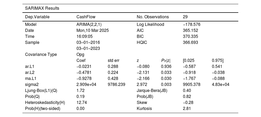
ARIMA model parameter selection

The cash flow model was optimized through systematic testing. Stationarity was assessed using the Augmented Dickey-Fuller (ADF) test: the original series (p = 0.82 > 0.05) and first-order differencing (p = 0.12 > 0.05) were non-stationary; however, second-order differencing achieved stationarity (p = 0.001 < 0.05), indicating d = 2.

The ACF and PACF plots suggested an AR(2) structure, as shown in Fig. 13 (The shaded area shows the confidence interval), the ACF plot showed a trailing pattern, while the PACF shows a second-order cutoff. An AR(2) model was initially attempted; however, further validation via Akaike Information Criterion (AIC) was required.

Fig. 13.

Autocorrelation and partial autocorrelation of cash flow.

The AIC comparisons identified ARIMA(2,2,1) as optimal (AIC=365.15) over alternatives such as ARIMA(2,2,0) (AIC=368.45), ARIMA(0,2,2) (AIC=367.92), and ARIMA(1,2,2) (AIC=366.78).

Residual diagnostics confirmed the model’s validity: the Ljung-Box test (p = 0.19> 0.05) showed no autocorrelation, and the Jarque-Bera test (p = 0.82 > 0.05) confirmed normal residuals. Therefore, we concluded that ARIMA(2,2,1) was optimal for the cash flow time series.

Debt Ratio Model ARIMA(1,1,1) Selection Process. Similar to Cash Flow ARIMA Model Selection, the debt ratio required first-order differencing (ADF p = 0.01 after differencing, d = 1) to attain stationarity (the original series p = 0.32 > 0.05). ACF/PACF plots indicated an AR(1) or MA(1) structure (Fig. 14).

Fig. 14.

Autocorrelation and partial autocorrelation of debt ratio.

The AIC comparisons favored ARIMA(1,1,1) (AIC=91.08) over other candidates (e.g., ARIMA(1,1,0): AIC=92.45, ARIMA(0,1,1): AIC = 93.12, ARIMA(2,1,1): AIC = 92.97).

Residual tests supported this choice, with the Ljung-Box test (p = 0.39 > 0.05) and Jarque-Bera test (p = 0.17 > 0.05) indicating no autocorrelation and near-normal residuals, respectively. Therefore, we concluded that ARIMA(1,1,1) was optimal for the debt ratio time series.

In summary, ARIMA(2,2,1) for cash flow and ARIMA(1,1,1) for debt ratio were rigorously validated, ensuring robust fit and reliable forecasting. The results of the cash flow and debt ratio data test are illustrated in Figs. 15 and 16, respectively. The ARIMA Model Test of the Cash Flow and debt ratio is detailed in the Appendix.

Fig. 15.

The cash flow data test results in ARIMA (2, 2, 1).

Fig. 16.

The debt ratio data test results in ARIMA (1, 1, 1).

Correspondingly, the forecasted cash flow and debt ratio trends are depicted in Figs. 17 and 18.

Fig. 17.

The cash flow forecast.

Fig. 18.

The debt ratio forecast.

Cash flow and debt ratio analysis

As shown in Fig. 17, SAIC’s cash flow experienced a significant decline starting in September 2022, primarily due to the adverse impact of the pandemic on its supply chain. This disruption directly affected the company’s liquidity position. According to the ARIMA(2, 2, 1) model’s forecast, the overall cash flow trend was expected to continue its downward trajectory from March 2023 to March 2024, albeit with occasional fluctuations. The model suggests that it would be challenging for SAIC to restore its cash flow to pre-pandemic levels in the near term.

Fig. 18 presents the forecasted debt ratio based on the ARIMA(1,1,1) model. The results indicate that SAIC’s gearing ratio is expected to stabilize at approximately 64 % over the coming year, with minor fluctuations. A debt ratio of 64 % is generally considered acceptable for capital-intensive industries such as manufacturing, as it provides the company with sufficient financial flexibility and borrowing capacity. At this level, SAIC could explore borrowing options to meet its working capital requirements, invest in new projects, or undertake debt restructuring to optimize its capital structure.

Strategic implications for BCF decision-making

Based on the forecasted trends in cash flow and debt ratio, it is evident that SAIC’s cash flow is likely to remain under pressure, while its debt ratio remains relatively stable. In light of these findings, we recommend that SAIC Motor consider securing a loan from the Bank of China in March 2023. This strategic decision could help mitigate the adverse effects of the pandemic on the company’s cash flow, ensuring the continuity of its day-to-day operations and supporting its long-term development objectives. Furthermore, by leveraging borrowing and financing, SAIC can optimize its capital structure, maintain financial flexibility, and enhance its market competitiveness.

Validation of the model

In March 2023, SAIC Motor entered into a partnership with the Bank of China, securing nearly 1 billion yuan in supplier financing.⁵ This real-world application of the model’s recommendations serves as a strong validation of its accuracy and practical relevance. The successful implementation of this financing strategy underscores the effectiveness of integrating financial indicators and time-series forecasting models in optimizing BCF decisions.

In conclusion, the extension examines how shifts in working capital influence the optimal BCF strategies through empirical investigation. We conducted a case study on SAIC to demonstrate that a firm’s optimal BCF decision is contingent on its current available working capital. In real-world scenarios, firms exhibit varying levels of working capital, and decision-making should not rely solely on the absolute value of operational funds. Instead, firms must evaluate their production capabilities, investment costs and sales costs of direct selling to assess their working capital position. Only then can they determine the most efficient BCF decision and cost-optimization strategy.

Conclusions

This study examines the combined effects of cost-reduction investment factors and direct selling costs on a supplier’s BCF and cost-reduction strategy, considering varying initial working capital levels. We also analyze how these factors influence the bank’s optimal interest rate. Our model incorporates three key elements: the cost-reduction factor, the bank’s interest rate, and direct selling costs. We evaluate equilibrium outcomes under different supply chain structures (i.e., with or without a direct selling channel) to determine the supplier’s optimal cost-reduction and BCF decisions. Additionally, we investigate how critical parameters affect decision-making for both the supplier and the bank.

The insights of this study extend beyond the immediate financial decisions of suppliers and banks. We also shed light on the broader dynamics of supply chain management and the role of financial institutions in supporting operational efficiency. For instance, banks can play a pivotal role in enabling cost-reduction efforts by offering tailored financing solutions that align with supplier needs and market conditions. Additionally, suppliers must consider external factors such as market demand, competition, and technological advancements when evaluating the potential impact of cost-reduction initiatives.

Moreover, the study highlights the importance of aligning cost-reduction strategies with the supplier’s overall financial health and operational goals. Suppliers with limited working capital must prioritize investments that yield the highest returns, whether through cost reduction, production expansion, or other efficiency-enhancing measures. Through a thorough evaluation of cost-reduction potential, fixed costs, and marginal costs, suppliers can determine the viability of investing in efficiency improvements and the need for external funding. Moreover, by showcasing strong cost-reduction prospects, suppliers may secure more favorable financing terms, such as lower interest rates.

In conclusion, our study provides a robust framework for understanding the complex interplay between financial constraints, production optimization, and cost-reduction strategies in supply chain management. By carefully analyzing their working capital levels, production needs, and cost structures, suppliers can make informed decisions on whether to seek external financing and whether to invest in cost reduction. These decisions not only impact the supplier’s financial health but also influence the overall efficiency and competitiveness of the supply chain. The theorem underscores the importance of aligning financial strategies with operational goals and highlights the transformative potential of bank financing in enabling production expansion and cost-reduction efforts.

This study explores cost-reduction investments and BCF decisions under single- and dual-channel structures at different working capital levels, suggesting several future research avenues: First, our analysis focuses on two primary entities: the supplier and the bank. Future research could incorporate the supplier’s Trade Credit Financing (TCF) into the model, allowing for a comparison between BCF and TCF. Second, our study assumes that the supplier is capital-constrained. Future research could introduce the management efficiency factors or more real-world factors, such as credit ratings, collateral, and macroeconomic policies, which affect bank rates, into the model. The demand uncertainties could also be considered so that the model captures the impact of economic cycles or policy changes.

CRediT authorship contribution statement

Jing Xia: Writing – original draft, Methodology, Investigation, Formal analysis. Yujie Xiao: Writing – review & editing, Validation, Supervision, Resources. Ling Yao: Writing – review & editing, Software, Resources, Investigation. Chuanxin Xia: Writing – review & editing, Methodology, Formal analysis.