Determining Parameters for Images Amplification by Pulses Interpolation

Abstract

This paper presents the implementation of a method for image samples interpolation based on a physical scanning model. It uses the theory to take digital image samples and to perform an implementation of such mechanism through software. This allows us to get the appropriate parameters for the images amplification using a truncated sampler arrangement. The shown process copies the physical model of image acquisition in order to incorporate the required samples for the amplification. This process is useful in the reconstruction of details in low resolution images and for images compression. The proposed method studies the conservation of high frequency in the high resolution plane for the generation of the amplification kernel. A new way of direct application of the physical model for scanning images in analytic mode is presented.

Resumen

Este trabajo muestra la aplicación de un método para la interpolación de muestras sobre una imagen basado en un modelo físico de digitalización de las mismas. Se utiliza la fundamentación teórica de muestreo de la imagen digital y se realiza una implementatión de dicho mecanismo a través de un software. Esto permite obtener los parámetros adecuados para amplificar las imágenes utilizando el arreglo de muestreo truncado. Se imita el procedimiento físico de obtención de la imagen y se incorporan las muestras requeridas para la amplificación. Este proceso es útil en la reconstrucción de detalles de imágenes de baja resolución y para la compresión de las mismas. El método propuesto estudia la conservación de las altas frecuencias en el plano de mayor resolución para la generación del núcleo de amplificación y presenta una nueva forma de aplicar directamente el modelo físico de escaneo de la imagen en modo analítico.

Introduction

This paper proposes a method for the construction of a pulse interpolation filter with maximum response amplitude at high spatial frequencies. This allows a better reconstruction of the details including the use of the characteristics of this type of amplification in order to achieve linear phase response in the edge transitions of the high resolution image. The preservation of edge information in an accurate frequency range gives a harmonious visual effect to the image and prevents the formation of blocks. This type of filter is used in the amplification, image reconstruction and simultaneously facilitates the compression process.

In some applications, as an imaging amplifier for Space-Multiplexed Optical Transmission (Ozdur el al., 2012) it is necessary to focus/collimate the light beam to the center of the bulk amplifier from the imaging systems (IS 1 and IS 2) of Figure 1 and then to couple back to the output fiber. The amplification effect of the bulk could be seeing as the electrical output of a more dense and sensible photo detector zone integrated over a period of time. During this period the light beam activates the resolution cells, and then the simulation of a photo detector sampling zone is useful to simulate the amplification effects.

Figure 1.

General schematic of the imaging amplifier. (MCF and MMF are the multicore and multimode fibers; IS is the imaging system

The medical-image analysis requires an understanding of sophisticated scanning modalities, constructing geometric models, building meshes to represent domains, and downstreaming biological applications. These four steps form an image-to-mesh pipeline (Levine et al., 2012).

The proposed method could be used as an edgepreserving interpolation method after the denoise process for noisy images. In some cases the image is first decomposed using the bilateral filter into the detail and base layers which represent the small and large scale features, respectively. The detail layer is adaptively smoothed to suppress the noise before interpolation and an edge-preserving interpolation method is applied to both layers, it is effective to employ denoising prior to the interpolation (Jong el al., 2010).

Some methods of interpolation, like the curvature interpolation method (CIM), study the edge composition of the low resolution image to interpolate the curvature to the high-resolution image domain. The CIM constructs the high-resolution image by solving a linearized curvature equation, incorporating the interpolated curvature as an explicit driving force (Hakran et al., 2011). Other regression-based image interpolation algorithms have been proposed in the literature, in which the objective functions are optimized by ordinary least squares (OLS). However, it has been shown that interpolation with OLS may have some undesirable properties from a robustness point of view: even small amounts of atypical values can dramatically affect the estimates (Liu el al., 2011).

This investigation tries to find the limits of quality in the high resolution image. The curvature content in the high-resolution image domain is studied using classical theory resources. A restricted interpolation system is made with spatial and window filters in order to increase the high frequency content. The proposed method constructs an interpolation kernel using the high frequency content at high-resolution image domain as an explicit driving force for the variation of the amplification kernel parameters. With this process, the optimal low-high resolution pair is found using the amplification kernel given by the Fourier transform of the truncated sampling arrangement (Papoulis, 1966). In the process filters as Butterworth (Pratt, 2001) and Canny (1986) are used in order to guide the construction of the interpolation kernel and to raise the high frequency content in the high resolution image.

Image sampling system

In a physical image sampling system the sampling arrangement should be of finite extent. The sampling pulses are of finite width and the image can be sub sampled with spectral overlap. Because of these, spurious spatial frequency components will be introduced into the reconstruction. This effect is called aliasing error (Brown, 1969; Helms and Thomas, 1962) and therefore it is necessary to explore the consequences of the nonideal sampling.

In the example of Figure 2, a thin beam of light goes through a photographic transparency of an ideal image. Passing light is collected in a condenser lens and is sent directly to a photo detector. The electrical output from the photo detector is integrated over a period of time during which the light beam activates a resolution cell. In this type of system is considered that even lens with perfect focus produces some blurring because of the diffraction limit of its opening (O’Neill, 1963).

Figure 2.

Scheme of the physical model scanning an image, taken from (Pratt, 2001)

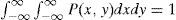
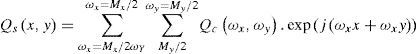
The sampled image is

where the arrangement of samples is

and is comprised of (2J + 1) (2K + 1) identical pulses P(x, y) arranged in a grid spacing (dx, dy). Symmetrical limits of summation are chosen, for notational simplicity, we assume that the sampling points are scaled.

For purposes of analysis it is assumed that the sampling function is generated by a finite array of Dirac deltas D_T(x, y) passing through a linear filter with impulse response P(x, y) then

Taking Equations 1 and 2 yields

The spectrum of the sampled image is given by

where P(w_x, w_y) is the Fourier transform of P(x, y).

The Fourier transform of the truncated sampling arrangement (Papoulis, 1966) is

This function, evaluated at the limit for large values of J and K, is converted into an array of Dirac deltas.

In an image reconstruction system, an image is reconstructed by interpolation of their samples. The interpolation waveforms selected as Sine function or Bessel generally extend over the entire field of the image (Pratt, 2001). If the arrangement is a discontinuous sampling, the reconstructed image will fail near their edges. However, the distance error is negligible in about 8 to 10 samples of Nyquist (Abramatic and Faugeras, 1982).

Modeling the interpolation system

In modeling the system a test image is taken for amplification by pulses interpolation. The aim is to achieve a new higher resolution image containing the highest fidelity with the original image. The process does not cause pixels block effect and maintains the continuity of phase in the Fourier transform of the result. This allows a smooth visual path. It contains the details in low-frequency areas and facilitates the compression. A convolution kernel (Abramatic and Faugeras, 1978; Pratt et al., 1982; Abramatic and Faugeras, 1982) is generated by the Fourier transform of the truncated sampling arrangement (8).

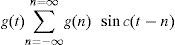
The space of the band limited functions in the frequency range ω ∈ [−π,π] is spanned by the infinite (yet countable) set of sine functions shifted by integers. Thus any such band limited function g(t) can be reconstructed from its samples at integer spacing.

Equations (7) and (9) yield

Now consider a spatial linear operator O{·}that produces an output image array

The term O{δ(t₁, t₂} for t_i = m_i - n_i + 1 is the response, at the output coordinate, to an input of one unit amplitude at coordinate (n₁, n₂). It is called the impulse response function array of the linear operator and is written as

The impulse response array can change form for each point (m₁, m₂) in the processed array Q(m₁, m₂). Following this notation, the finite area superposition operation is defined as

This expresses the finite-area superposition operation in the left-justified form in which the input and output arrays are aligned at their upper left corners. It is often notation-wise convenient to utilize a definition in which the output array is centered with respect to the input array. This definition of centered superposition is given by

The limits of the summation are

In Figure 4 the examination of the indices of the impulse response array at their extreme positions indicates that M = N + L −1, and hence the processed output array Q is of larger dimension than the input array F.

Figure 3.

Scheme of the interpolation function, only one coordinate

Figure 4.

Relationships between input data, output data, and impulse response arrays for finite-area superposition; centered array definition taken from (Pratt, 2001)

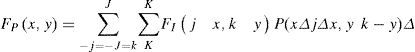
In the interpolation system, the input array F is the low resolution image of (N_x, N_y). Then, using (7), (8) and (13), the output data array Q_c(j₁, j₂) is obtained. Using (10), the samples of D_t(ω_x, ω_y) for the interval in which ω ∈ [-π, π] are inserted. Figure 3 shows how for Δx = 1 and Δy = 1, L_y = 2 • K and L_x = 2 • J.

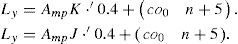
where J’ and K’ are the dimensions of the low resolution image, this is, the input array F.(24)

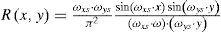
Obtaining the impulse response function array in function of the exploration parameters inc and co.

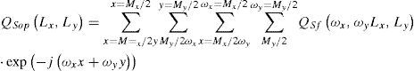
Evaluating the expression for ω_x ∈[-π, π], ω_y ∈ [-π, π] and using (19) we obtain the output array Q_c(j₁, j₂), which has dimensions (M_x, M_y), where

Then the inverse transformation of the output array gives the high resolution image

In order to define the parameters inc and co of equations (15) and (16), the high frequency estimate over Q_s(x, y) is applied. Applying a Butterworth high pass filter (Pratt, 2001) to less than 5 pixel elements

Spatial filters for the edge detection over the high resolution image are used in another case. A Canny type filter is applied (Canny, 1986) in order to estimate the amount of edge content and to restrict the parameters A_mp, inc and co of equations (15) and (16). In this case the implementation of the Canny operator gives

Then the appropriate values of L_y and L_x can be found in both cases by

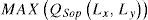
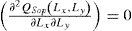
Due to the complexity of the formulation, no analytic solution has been found, but a variational approach has been developed. Defining a fixed value for the large resolution modifier A_mp = 1.1, the maximum responses of high frequencies are found by the output of the filter only for some combination values of the scan parameters inc and co. The high frequencies response of the high resolution image using the Butterworth filter of the equation (20) is shown in Figure 5.

Figure 5.

Graphic parameters scan for the output of the filter type ‘Butterworth’ (Pratt, 2001), order 5 for

Figures 6 or 8 show how a periodicity exists in each row; for example, if inc = 0.4 the best result appears every 5 figures and the resolution of the output image increases according to equation (22). For a good result, if inc = 0.4 then co = co₀+ n • 5 when co₀ = 4, equations (15) and (16) get the exact dimensions. But the best result for the Butterworth guide comes from Table 1, co = 19, inc = 0.4 where this pattern combination gives us the maxim conservation value of the frequency range of the filter (Figure 9).

Figure 6.

Map of parameter selection for high frequency levels of high pass filter type Butterworth (Pratt, 2001) order 5 for less than 5 pixel elements over the results of the interpolation filter

Figure 7.

High resolution image whit co = 19 and inc = 0.4, and the guide of Butterworth (Pratt, 2001), order 5 for less than 5 pixel elements

Figure 8.

Map of high resolution images obtained by the interpolation kernel varying parameters

Table 1.

High frequency magnitudes after the adjustment process of the amplification kernel. Sum of units of least energy change per pixel result of the high pass filter type Butterworth (Pratt, 2001), order 5 for less than 5 pixel elements

CO	inc=0.1	inc=0.2	inc=0.3	inc=0.4	inc=0.5
1	383928567,687645	270095037,508266	169198039,912090	102292472,923475	125127676,957232
2	265336827,105852	94633549,2094335	129772765,750036	90655325,4611820	270138137,174281
3	157399882,781851	126253386,468731	162435251,425276	502431645,964924	802194399,470288
4	78063421,3240791	86932171,0105289	502020648,615752	829747255,982912	514671554,508373
5	105195160,856602	265515683,841707	798848643,137986	513236839,238852	123753730,390564
6	115601427,542619	501701038,483607	733999530,952639	99774761,6931317	269928660,113030
7	100589995,469657	725245838,189243	390671166,003094	90410729,5035506	809589665,431580
8	71483800,9070080	827297391,509886	95648619,2983738	507855576,795838	518622467,896560
9	152354026,996521	734377407,381142	113652216,857252	836032023,851749	123233632,319536
10	260325092,865537	509908457,350087	268612928,958653	516477468,586911	273207463,923044
11	379071451,392629	268192909,414039	628325957,888577	96690369,9074624	815764892,457752
12	500332472,602403	78953076,5124871	836469798,355744	88809521,0980179	521890543,565737
13	622010395,730627	116933760,026838	636913647,263801	513320418,457530	120472385,889034
14	727068317,400424	72255954,4438813	271311592,423545	845105285,844718	274630252,046820
15	802300090,381683	263321971,361200	107661335,427739	521099266,043549	824783465,459286
16	830828568,075156	506052996,661072	73031823,6914790	80953870,6143567	526345829,248504
17	807684329,368176	735114700,534598	387577748,801602	73733511,8314926	110166690,342695
18	734377407,381142	839728077,836381	743205085,474997	517243362,064077	271945387,044346
19	629973217,428392	742412308,021623	824984133,789389	856772169,300154	836016262,233911
20	383928567,687645	270095037,508266	169198039,912090	102292472,923475	125127676,957232

Figure 9.

The original test image has 226 × 182 pixels

In order to obtain a new vertical resolution, from 182 to 1800 pixels

less than 5 pixel elements, increment (inc) differentiated per colors and sample number (co) identify the number of measurements taken for each increment

Figures 7 and 10 show how a loss of the high frequency content occurs. The application of the interpolation kernel with the Butterworth filter guide produces this effect. This filter does not give the maximum values of frequency of contour information.

Figure 10.

High resolution ¡mage using the periodic pattern of Figure 8 for the parameters calculation in a specific amplification from 182 × 226 to 1800 × 2235 pixels

The Canny method finds edges by looking for the local maximum of the image gradient. The gradient is calculated using the derivative of a Gaussian filter. The method uses two thresholds to detect strong and weak edges, and includes the weak edges in the output only if they are connected to strong edges. This method is therefore less likely than the others to be deceived by noise, and more likely to detect true weak edges.

The classical separable sine impulse response function array (Pratt, 2001) is

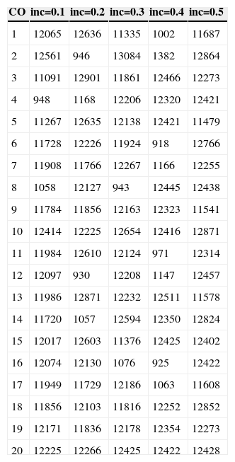
Compare, in Figure 13, the results of the sine separable interpolation (30) and the application of the impulse response function array (20) restricted by the Canny filter over the first column of the high resolution image. Figure 11 shows the periodicity and the peaks useful for the amplification. The map of figure 12 has localized a zone where exist a maximum value obtained from the Table 2, with co = 10 and inc = 0.5. Figure 14 shows how the high resolution image maintains the original contrast. This figure has better conserved contour information than the one obtained with the classic interpolation using the impulse response function array (30).

Figure 11.

Graphic parameters scan for the output of Canny filter (Canny, 1986) increment (inc) differentiated by colors and sample number (co) identify the number of measurements taken for each increment

Figure 12.

Map of parameters selection for high frequency levels of high pass filter type ‘Canny’ (Canny, 1986) applied over the results of the interpolation filter

Figure 13.

Comparison of the sine separable interpolation (30) and the application of the impulse response function array (20) restricted by the Canny filter over the first column of the high resolution image with A_mp = 1.1, inc = 0.5 and co = 18

Table 2.

High frequency magnitudes after the adjustment process of the amplification kernel. Sum of units of least energy change per pixel resulting from high pass filter type ‘Canny’ (Canny, 1986)

CO	inc=0.1	inc=0.2	inc=0.3	inc=0.4	inc=0.5
1	12065	12636	11335	1002	11687
2	12561	946	13084	1382	12864
3	11091	12901	11861	12466	12273
4	948	1168	12206	12320	12421
5	11267	12635	12138	12421	11479
6	11728	12226	11924	918	12766
7	11908	11766	12267	1166	12255
8	1058	12127	943	12445	12438
9	11784	11856	12163	12323	11541
10	12414	12225	12654	12416	12871
11	11984	12610	12124	971	12314
12	12097	930	12208	1147	12457
13	11986	12871	12232	12511	11578
14	11720	1057	12594	12350	12824
15	12017	12603	11376	12425	12402
16	12074	12130	1076	925	12422
17	11949	11729	12186	1063	11608
18	11856	12103	11816	12252	12852
19	12171	11836	12178	12354	12273
20	12225	12266	12425	12422	12428

Figure 14.

High resolution image for co = 10 and inc = 0.5, oriented by ‘Canny’ filter (Canny, 1986)

In Figure 15, an integer number multiplier is used in order to construct a more dense mesh of the interpolation kernel (20). The parameters in Table 2 for the maximum high frequency response in the high resolution image are used.

Figure 15.

Left side, details of the test image using the interpolation filter, there is a 1 550% amplification of the original image detail from 25 × 30 to 387 × 464 pixels taken adequate increase step from the right side of equations (15) and (16), original image detail of 25 × 30 pixels

In the case of Figure 15, from equation (15)

And from equation (16)

Discussion and analysis of results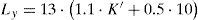

The investigation shows the main aspects of the interpolation with restriction for the amplification. For instance, which is the goal in the amplification process? What filter could be the guide for the parameters in the construction of the response impulse function or amplification kernel? The Butterworth filter takes in consideration a range of high frequencies, in the case for Δx = 5 pixels, but the main trouble in the interpolation is the contour conservation or high frequencies, that are just over π. The results of amplification guide by Butterworth give possible combination of parameters for equations (15) and (16) in a range of frequencies. In order to have better results it is necessary to use a filter directly related with the contour information of the image. The edge detectors are developed with a robust capacity for the detection. One famous detector is the Canny filter (Canny, 1986).Then the high frequencies of the interpolation output are related to the impulse response function array using the Canny filter. We found the adequate parameters inc and co in order to make the interpolation kernel, increase the high frequency content in the high resolution image.

Other aspect is the control of the coordinates of amplification of the filter. It is shown in Figures 6 or 8 how periodicities exist in each inc row. The argument of the sine components of the impulse response function array in function (20) are near π/2 with the exploration parameters inc = 0.4 and co = co₀+ n • 5 for the contour interpolation. The amplification suited under this condition takes the dimensions desired using (15) and (16). Figure 10 is an exact amplification to the precise coordinates. But this process gives losses with the guide of the Butterworth filter. When controlling the amplification it is preferable, for the conservation of high frequency content in the high resolution plane, to find a local maximum using the Canny filter. A whole number is used as multiplier to increase the interpolation kernel dimensions. Another important topic is the comparison applying the classical separable sine impulse response function array (30) and the interpolation results with the impulse response function array (20) constrained by the neighbor detector filter Canny type. It is shown how the restriction increases the range of the pixels values doing a contribution to the high frequency conservation in the high resolution plane. In the last case it is analyzed how the guide of Canny is useful to construct an interpolation kernel in order to obtain a very high resolution image taking only maximum local values in a range. The parameters, when the high frequency content increases, represent the adequate amount of sampler components in the impulse response array S(x, y) of equation (1) for the interpolation. The sampler components are more numerous than the samples of the original image for the interpolation, but the position of these are in the active zone of the resolution cell of the physical scan model and consequently over the valid values of the pixels in the original image and not between. Then the interpolation kernel increases by a whole number multiplier for the adequate parameters A_mp, inc and co giving a high frequency maximum in an initial range. Using this mode we obtained a very high resolution image. The high frequency content in the high resolution plane was retained. Figure 15 shows how this effect occurs over an amplification of the 1550% in each coordinate.

Conclusions

This paper shows an effective way for optimizing a pulse interpolation filter in order to obtain the best visual result for the required amplification rate. The proposed amplification method retains the high frequency content and does not produce pixels block effect. A new way of relationship between the constructions of the interpolation kernel and the guide of classic filters is shown in order to increase the high frequency content in the high resolution image. The restriction of the interpolation process using high pass filters increases the range of the pixels values doing a contribution to the high frequency conservation in the high resolution plane. A Canny detector is more effective than the Butterworth high pass filter for the high frequency conservation in the amplification. The characterization of the filter is necessary for the efficient application in different processes of restoration and reconstruction, preserving the characteristics of the primary image. The proposed method makes adequate amplification filters for specific purposes in the field of digital photo restoration and image and video compression.