


The aims of the present study were to determine the level of sexual dimorphism among two populations, one from Mexico City and the other from Hidalgo, Mexico, as well as the development of discriminant functions for gender assessment using the mandible, for human identification.
Materials and methodsTwo samples of mandibles were analysed morphometrically, one from Mexico City (Colección-UNAM) (MEX), and the other from Santa María Xigui, Alfajayucan, Hidalgo, México (XIG). The sample MEX consisted of 108 mandibles (75 male and 33 female), and XIG sample with 56 mandibles (33 female and 30 male), with a mean age between 49.2 and 55.1 years old. Eighteen measurements were taken to create four discriminant functions for gender estimation for each sample.
ResultsThe differentiation pattern among populations (samples) was the same. Nevertheless, there were differences between them, with a higher degree of sexual difference in XIG.
The discriminant functions, developed for both populations, achieved a correct classification in between 76.4 and 84%, respectively.
ConclusionThe XIG sample showed greater sexual dimorphism than the MEX sample, with longer mandibles and higher and elongated chins.
The discriminant functions generated in this study, present higher classification percentages than the other existing proposals. Furthermore, being developed from the contemporary population, they can be used in forensic contexts for human identification, with complete or fragmented/incomplete remains.
El presente trabajo tuvo como objetivos: conocer el grado de dimorfismo sexual entre una población de la Ciudad de México y otra de Hidalgo, México; y el desarrollo de funciones discriminantes para la estimación de sexo por medio de la mandíbula, para identificación humana.
Material y métodosSe analizaron morfométricamente mandíbulas de dos muestras, una procedente de la Ciudad de México (MEX) (Colección-UNAM) y otra de Santa María Xigui, Alfajayucan, Hidalgo, México (XIG). La muestra MEX consistió en 108 mandíbulas (75 masculinos y 33 femeninos) y en la muestra XIG se utilizaron 56 mandíbulas (33 femeninos y 30 masculinos), con una edad media entre 49,2 y 55,1 años. Se tomaron 18 medidas mandibulares y se desarrollaron cuatro funciones discriminantes para estimar el sexo con cada muestra.
ResultadosSe observó el mismo patrón de diferenciación en ambas poblaciones, no obstante se presentaron diferencias entre estas, ya que se demostró que existe mayor grado de diferencias sexuales en XIG.
Las funciones discriminantes desarrolladas para ambas poblaciones, alcanzaron entre el 76,4 y 84% de clasificación sexual correcta.
ConclusionesLa muestra XIG presentó mayor dimorfismo sexual que la muestra MEX, con mandíbulas más alargadas y mentones altos y alargados.
Las funciones discriminantes del presente trabajo presentan porcentajes de clasificación mayores a los de las demás propuestas existentes. Y al ser desarrolladas a partir de población contemporánea, pueden ser utilizadas en contextos forenses para identificación humana con restos completos o fragmentados y/o incompletos.
Determining gender from human skeletal remains is a procedure of fundamental importance both for human identification in forensic anthropology and in the bioarchaeological context.
The skull and pelvic bones have been considered as the best bone elements for determining gender in an individual.1–3 However, when such structures are not available, the bones of the postcranial skeleton and the mandible can provide valuable information regarding a person's gender.4
For Mexico's contemporary population, different methods have been developed which, based on the analysis of discriminant functions, make it possible to determine an individual's gender from their skeletal remains. Examples are suggestions for long bones,5–9 scapula,10 patella,11,12 pelvis,9,13 carpal bones14 and metacarpals and metatarsals.15 There have also been studies to determine gender from the mandibles of pre-Hispanic16 and indigenous9 Mexican populations.
Previous research suggests that discriminant functions should be population-specific, and recent studies comparing different populations have shown that there are significant differences in mandibular morphology and size between genders,17–19 and even intrapopulation changes in sexual dimorphism.20 Our study therefore has a dual objective: to determine whether or not there are differences in the degree of sexual dimorphism between the populations of Mexico City and Santa María Xigui, Hidalgo; and to develop discriminant functions for determining gender in a population-specific way.
Materials and methodTo perform the study, two samples were analysed, the first one from Mexico City and the second from the State of Hidalgo, Mexico.
The first sample belongs to the Bone Collection of the Department of Anatomy's Physical Anthropology Laboratory in the Faculty of Medicine at UNAM (Universidad Nacional Autónoma de México [National Autonomous University of Mexico]) (Colección-UNAM). The Colección-UNAM (MEX) is made up of the skeletons of unclaimed corpses, used for dissection practice. Most of the corpses have ante-mortem data, such as gender and age, and in some cases the name and cause of death. They come from the Institute of Forensic Sciences (Instituto de Ciencias Forenses, INCIFO), as well as Centres for Assistance and Social Integration (Centros de Asistencia e Integración Social, CAIS) belonging to the Institute of Assistance and Social Integration and Mexico City Health Service hospitals.
The second sample came from the cemetery of the town of Santa María Xigui (XIG) in the Alfajayucan district of the State of Hidalgo, Mexico. This town is of Otomí origin and is one of the nine regions that make up the Mezquital Valley.
The material was obtained on loan with the consent of the relatives during work to relocate the cemetery, carried out in December 2013. Through the information provided by the relatives, the gender of each individual was known; information about age was not obtained for the whole sample, but all cases were adults.
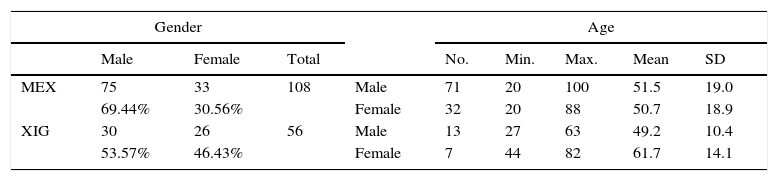
In the first sample, 108 mandibles were analysed (30.56% female and 69.44% male). For the first sample from Mexico City (MEX), the ages of 71 of the total of 75 males were obtained, the minimum age being 20 and the maximum 100, with a mean age of 55.1 and standard deviation of 19.0 years. For the females, the ages of 32 of the 33 analysed were known, the minimum age being 20 and maximum 88, with a mean age of 50.7 and standard deviation of 18.9 years. The dates of death of the individuals were in the period 1990–2010 (Table 1).
Composition of the sample by age and gender.
| Gender | Age | ||||||||
|---|---|---|---|---|---|---|---|---|---|
| Male | Female | Total | No. | Min. | Max. | Mean | SD | ||
| MEX | 75 | 33 | 108 | Male | 71 | 20 | 100 | 51.5 | 19.0 |
| 69.44% | 30.56% | Female | 32 | 20 | 88 | 50.7 | 18.9 | ||
| XIG | 30 | 26 | 56 | Male | 13 | 27 | 63 | 49.2 | 10.4 |
| 53.57% | 46.43% | Female | 7 | 44 | 82 | 61.7 | 14.1 | ||
Colección-UNAM [UNAM Collection] (MEX) and Santa María Xigui (XIG). Max.: maximum; Min.: minimum; No.: sample number; SD: standard deviation.
In the second sample, 56 mandibles were analysed (46.43% female and 53.57% male). In Santa María Xigui (XIG), ages were obtained for 13 of the 30 male individuals analysed, the minimum age being 27 and maximum 63, with a mean of 49.2 and a standard deviation of 10.4 years. For the females, ages were recorded for seven of the 33, the minimum age being 44 and the maximum 82, with a mean of 61.7 and a standard deviation of 14.1 years. The dates of death for this sample were in the period 1960–2010 (Table 1).
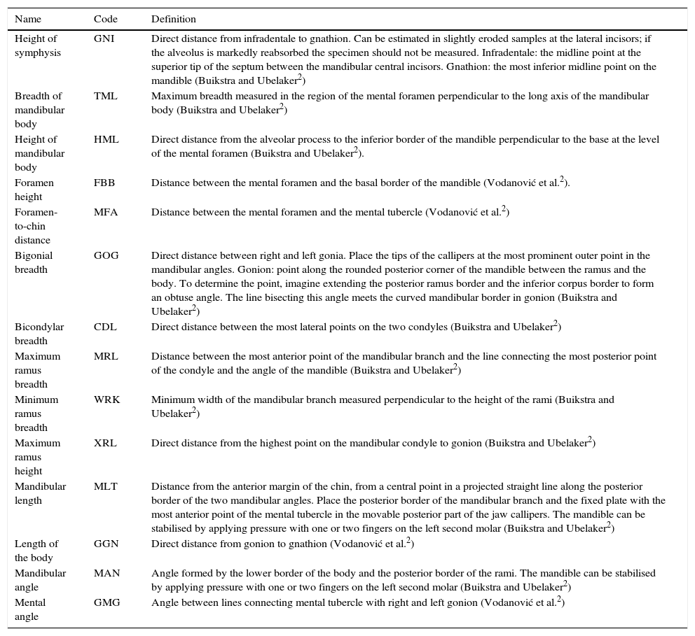
For the morphometric analysis, we selected mandibles of mature subjects, in good condition, with no pathologies (e.g. trauma, degenerative processes and severe periodontal disease) or post-mortem changes. We took 14 mandible measurements in mm, following the Buikstra and Ubelaker criteria2 and four measurements as proposed by Vodanović et al.,21 with digital electronic callipers (Scala©) and jaw callipers (Paleo-Tech concept©) (Fig. 1 and Table 2).

Mandible variables CDL: bicondylar breadth; FBB: foramen height; GGN: length of the body; GMG: mental angle; GNI: height of symphysis; GOG: bigonial breadth; HML: height of mandibular body; MAN: mandibular angle; MFA: foramen-to-chin distance; MLT: mandibular length; MRL: maximum ramus breadth; TML: breadth of mandibular body; WRK: minimum ramus breadth; XRL: maximum ramus height.
Definition of mandibular measurements.
| Name | Code | Definition |
|---|---|---|
| Height of symphysis | GNI | Direct distance from infradentale to gnathion. Can be estimated in slightly eroded samples at the lateral incisors; if the alveolus is markedly reabsorbed the specimen should not be measured. Infradentale: the midline point at the superior tip of the septum between the mandibular central incisors. Gnathion: the most inferior midline point on the mandible (Buikstra and Ubelaker2) |
| Breadth of mandibular body | TML | Maximum breadth measured in the region of the mental foramen perpendicular to the long axis of the mandibular body (Buikstra and Ubelaker2) |
| Height of mandibular body | HML | Direct distance from the alveolar process to the inferior border of the mandible perpendicular to the base at the level of the mental foramen (Buikstra and Ubelaker2). |
| Foramen height | FBB | Distance between the mental foramen and the basal border of the mandible (Vodanović et al.2). |
| Foramen-to-chin distance | MFA | Distance between the mental foramen and the mental tubercle (Vodanović et al.2) |
| Bigonial breadth | GOG | Direct distance between right and left gonia. Place the tips of the callipers at the most prominent outer point in the mandibular angles. Gonion: point along the rounded posterior corner of the mandible between the ramus and the body. To determine the point, imagine extending the posterior ramus border and the inferior corpus border to form an obtuse angle. The line bisecting this angle meets the curved mandibular border in gonion (Buikstra and Ubelaker2) |
| Bicondylar breadth | CDL | Direct distance between the most lateral points on the two condyles (Buikstra and Ubelaker2) |
| Maximum ramus breadth | MRL | Distance between the most anterior point of the mandibular branch and the line connecting the most posterior point of the condyle and the angle of the mandible (Buikstra and Ubelaker2) |
| Minimum ramus breadth | WRK | Minimum width of the mandibular branch measured perpendicular to the height of the rami (Buikstra and Ubelaker2) |
| Maximum ramus height | XRL | Direct distance from the highest point on the mandibular condyle to gonion (Buikstra and Ubelaker2) |
| Mandibular length | MLT | Distance from the anterior margin of the chin, from a central point in a projected straight line along the posterior border of the two mandibular angles. Place the posterior border of the mandibular branch and the fixed plate with the most anterior point of the mental tubercle in the movable posterior part of the jaw callipers. The mandible can be stabilised by applying pressure with one or two fingers on the left second molar (Buikstra and Ubelaker2) |
| Length of the body | GGN | Direct distance from gonion to gnathion (Vodanović et al.2) |
| Mandibular angle | MAN | Angle formed by the lower border of the body and the posterior border of the rami. The mandible can be stabilised by applying pressure with one or two fingers on the left second molar (Buikstra and Ubelaker2) |
| Mental angle | GMG | Angle between lines connecting mental tubercle with right and left gonion (Vodanović et al.2) |
Particular care is recommended with measurements at the alveolar ridge (HML and GNI) as alveolar resorption can be a source of measurement error.
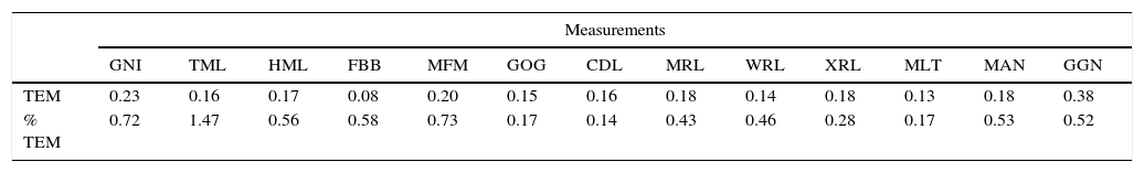
In order to eliminate sources of error, all measurements were performed by a single observer in a continuous session. Additionally, the technical error of measurement (TEM)22 was estimated in a random subsample of 30 individuals.
The univariate statistical analyses performed from the measurements of the mandibles of both samples were: (1) descriptive statistics; (2) Shapiro–Wilk normal distribution test (data not shown in this paper); and (3) Student's-t test to check for significant differences between the measurements for each gender, and Levene's F test for equality of variances.
In order to evaluate differences in the degree of sexual dimorphism between populations, we used the t-test derived by Relethford and Hodges.23
Lastly, the discriminant analysis was performed, obtaining the percentage of variance explained, the eigenvalues acquired, Wilks’ Lambda, the standardised coefficients and the percentage summary of the probability of belonging to a group.
The discriminant analysis was performed considering the step-by-step inclusion method, whereby the discriminant functions were constructed from the variables considered within the analysis as significant and which amassed the highest percentage in the reclassification.
All statistical analyses were performed using SPSS© v.15.0 (https://www.ibm.com) and PAST© v.1.8824 software.
ResultsThe TEM showed minimum values of 0.14% in the bicondylar breadth (CDL) and a maximum of 1.47% for breadth of mandibular body (TML) (Table 3).
Table 4 shows the mean values, variation values and the tests of comparison of means between genders for each of the skeletal series (Colección-UNAM [MEX] and Santa María Xigui [XIG]). The Shapiro–Wilk test showed that each variable had normal distribution (p<0.05).
Mandibular measurement (mm) statistics.
| Mexico (MEX) | |||||||||||||||||
|---|---|---|---|---|---|---|---|---|---|---|---|---|---|---|---|---|---|
| Male | Female | ||||||||||||||||
| No. | Mean | Median | SD | Min. | Max. | No. | Mean | Median | SD | Min. | Max. | Levene's-F | Sig. | Student's-t | df | Sig. | |
| GNI | 75 | 31.97 | 31.81 | 3.89 | 21 | 40 | 33 | 29.97 | 29.93 | 4.76 | 20 | 39 | 2.57 | 0.1116 | 2.30 | 106 | 0.0231 |
| TML | 75 | 11.13 | 11.06 | 1.33 | 8 | 14 | 33 | 10.94 | 10.96 | 1.28 | 9 | 14 | 0.01 | 0.9180 | 0.68 | 106 | 0.5005 |
| HML | 75 | 29.43 | 29.90 | 3.53 | 21 | 35 | 33 | 28.42 | 28.71 | 3.31 | 22 | 34 | 0.16 | 0.6944 | 1.39 | 106 | 0.1679 |
| FBB | 75 | 14.41 | 14.41 | 1.32 | 11 | 19 | 33 | 13.79 | 14.04 | 1.57 | 10 | 17 | 1.55 | 0.2165 | 2.12 | 106 | 0.0367 |
| MFA | 75 | 27.57 | 27.82 | 2.04 | 23 | 32 | 33 | 27.03 | 26.72 | 1.85 | 24 | 30 | 2.12 | 0.1480 | 1.30 | 106 | 0.1953 |
| GOG | 75 | 90.06 | 90.11 | 5.41 | 77 | 103 | 33 | 84.80 | 85.05 | 4.22 | 78 | 93 | 2.85 | 0.0944 | 4.95 | 106 | 0.0000 |
| CDL | 75 | 116.85 | 116.91 | 5.81 | 99 | 129 | 33 | 111.33 | 111.30 | 6.11 | 98 | 127 | 0.16 | 0.6893 | 4.47 | 106 | 0.0000 |
| MRL | 75 | 43.44 | 43.57 | 3.06 | 36 | 51 | 33 | 41.46 | 40.96 | 2.93 | 36 | 49 | 0.44 | 0.5063 | 3.12 | 106 | 0.0023 |
| WRK | 75 | 32.19 | 31.71 | 2.57 | 26 | 37 | 33 | 30.87 | 30.77 | 2.38 | 25 | 35 | 2.05 | 0.1550 | 2.52 | 106 | 0.0132 |
| XRL | 75 | 68.91 | 69.16 | 4.98 | 56 | 81 | 33 | 64.08 | 64.09 | 4.68 | 56 | 75 | 0.01 | 0.9408 | 4.73 | 106 | 0.0000 |
| MLT | 75 | 79.87 | 79.00 | 4.23 | 70 | 90 | 33 | 78.27 | 79.00 | 4.58 | 70 | 88 | 0.88 | 0.3512 | 1.76 | 106 | 0.0817 |
| GGN | 75 | 76.07 | 75.97 | 4.35 | 65 | 85 | 33 | 72.97 | 72.61 | 4.79 | 63 | 85 | 0.49 | 0.4850 | 3.30 | 106 | 0.0013 |
| MAN | 75 | 123.28 | 123.00 | 6.98 | 108 | 141 | 33 | 124.82 | 126.00 | 7.07 | 109 | 139 | 0.00 | 0.9550 | −1.05 | 106 | 0.2956 |
| GMG | 75 | 73.04 | 73.00 | 4.94 | 59 | 85 | 33 | 71.06 | 72.00 | 4.42 | 64 | 81 | 0.04 | 0.8446 | 1.98 | 106 | 0.0506 |
| Xigui (XIG) | |||||||||||||||||
|---|---|---|---|---|---|---|---|---|---|---|---|---|---|---|---|---|---|
| Male | Female | ||||||||||||||||
| No. | Mean | Median | SD | Min. | Max. | No. | Mean | Median | SD | Min. | Max. | Levene's-F | Sig. | Student's-t | df | Sig. | |
| GNI | 30 | 36.54 | 36.33 | 2.81 | 32 | 44 | 26 | 32.70 | 33.84 | 2.55 | 27 | 36 | 0.04 | 0.8459 | 5.33 | 54 | 0.0000 |
| TML | 30 | 12.36 | 11.93 | 1.88 | 8 | 16 | 26 | 11.61 | 11.76 | 1.16 | 9 | 14 | 5.31 | 0.0250 | 1.75 | 54 | 0.0858 |
| HML | 30 | 32.74 | 32.09 | 2.25 | 29 | 37 | 26 | 29.37 | 29.77 | 2.29 | 25 | 33 | 0.13 | 0.7204 | 5.54 | 54 | 0.0000 |
| FBB | 30 | 15.92 | 16.05 | 1.64 | 12 | 20 | 26 | 14.47 | 14.57 | 1.27 | 12 | 16 | 1.01 | 0.3197 | 3.66 | 54 | 0.0006 |
| MFA | 30 | 28.41 | 27.99 | 2.05 | 25 | 34 | 26 | 26.60 | 26.53 | 1.28 | 24 | 30 | 5.72 | 0.0203 | 3.90 | 54 | 0.0003 |
| GOG | 30 | 92.22 | 90.99 | 5.16 | 81 | 104 | 26 | 86.71 | 87.15 | 4.56 | 79 | 95 | 0.19 | 0.6668 | 4.21 | 54 | 0.0001 |
| CDL | 30 | 123.96 | 124.90 | 4.03 | 115 | 132 | 26 | 119.41 | 119.06 | 3.62 | 113 | 126 | 0.29 | 0.5915 | 4.41 | 54 | 0.0000 |
| MRL | 30 | 45.06 | 45.03 | 3.26 | 40 | 51 | 26 | 44.05 | 44.22 | 3.49 | 39 | 52 | 0.19 | 0.6659 | 1.12 | 54 | 0.2668 |
| WRK | 30 | 34.36 | 34.64 | 2.38 | 30 | 39 | 26 | 32.95 | 32.03 | 3.31 | 26 | 41 | 3.24 | 0.0773 | 1.85 | 54 | 0.0704 |
| XRL | 30 | 69.13 | 69.63 | 3.45 | 60 | 77 | 26 | 63.30 | 63.48 | 5.19 | 49 | 73 | 2.97 | 0.0904 | 5.01 | 54 | 0.0000 |
| MLT | 30 | 80.03 | 80.50 | 4.20 | 73 | 89 | 26 | 76.00 | 75.50 | 3.48 | 69 | 83 | 1.77 | 0.1891 | 3.88 | 54 | 0.0003 |
| GGN | 30 | 75.90 | 75.09 | 4.17 | 69 | 86 | 26 | 71.65 | 70.76 | 3.63 | 65 | 79 | 0.81 | 0.3721 | 4.03 | 54 | 0.0002 |
| MAN | 30 | 121.67 | 121.00 | 6.78 | 107 | 135 | 26 | 123.58 | 124.00 | 5.82 | 110 | 136 | 0.34 | 0.5602 | −1.12 | 54 | 0.2669 |
| GMG | 30 | 75.50 | 75.00 | 4.89 | 66 | 87 | 26 | 74.69 | 74.00 | 4.15 | 66 | 82 | 0.50 | 0.4815 | 0.66 | 54 | 0.5118 |
Descriptive statistics for Mexico City, Colección-UNAM [UNAM Collection] (MEX) and Santa María Xigui (XIG). SD: standard deviation; Max.: maximum; Min.: minimum; No.: sample number; Sig.: significance.
Means that are significantly different are shown in bold and italics.
In general terms, the same pattern of differentiation can be seen in both populations, as the male mandibles are larger in breadth, length and height. However, this was not the case with the mandibular angle, where the females had higher values. Contrary to expectations, the angular measurements (MAN and GMG) did not show significant differences between genders (p>0.05).
Although the Student's-t test showed significant differences (p<0.05) in the measurements of the variables GNI, FBB, GOG, CDL, XRL and GGN in both MEX and XIG, the Relethford and Hodges t-test23 showed that there was a greater degree of sexual difference in XIG than in MEX, with XIG, in general, showing greater robustness. It is thus possible to appreciate that the differences in XIG individuals with respect to MEX individuals are mainly located in the chin region and mandible length, i.e., tall, elongated chins and longer mandibular bodies (Fig. 2).
. The variables HML, FBB, MFA and MLT, are statistically significant >0.05, i.e. these measurements show that the chin of the XIG population is longer and taller, and the mandibular body is longer, compared to MEX.")
Graph corresponding to the degree of sexual dimorphism between populations (Relethford and Hodges23). The variables HML, FBB, MFA and MLT, are statistically significant >0.05, i.e. these measurements show that the chin of the XIG population is longer and taller, and the mandibular body is longer, compared to MEX.
From the Relethford and Hodges t-statistic,23 a pattern was observed that showed differences in the degree of sexual dimorphism between groups; as a consequence of which the discriminant analysis was performed independently for each population (MEX and XIG).
Four discriminant functions were obtained, the first including all the variables; the second in which the mandibular angles were omitted; a third that excluded all variables that showed no significant differences between genders in the univariate analysis (p<0.05); and the fourth in which the step-by-step inclusion method was used and which for MEX considered two variables (GOG and XRL) and for XIG three variables (HML, CDL and GGN).
In the first discriminant function (F1) where all variables were considered, a probability of correct classification in relation to the reference group of 78.1% was obtained. For the second discriminant function (F2), 78.7% was obtained in correct gender assignment. Like F1, the second function required an anatomically complete mandible in order to calculate the equation. With the third function (F3), the percentage correctly allocated was 76.4%. The fourth discriminant function (F4) obtained a correct classification percentage of 76.7%. It should be noted that for this function two of the 14 variables were considered. F4 can be used as an alternative in fragmented mandibles, which is of fundamental importance in forensic contexts (Table 5).
Discriminant functions (F) for gender determination from the mandible in the Mestizo population of Mexico City (MEX) and indigenous population (XIG) of Santa María Xigui.
| MEX | XIG | |||||||
|---|---|---|---|---|---|---|---|---|
| Variables | F4 | F3 | F2 | F1 | F4 | F3 | F2 | F1 |
| GNI | 0.3461 | 0.3576 | 0.3612 | 0.4336 | 0.4212 | 0.4582 | ||
| TML | −0.0824 | −0.0876 | 0.0851 | 0.0944 | ||||
| HML | −0.4969 | −0.4939 | −0.4825 | 0.6565 | 0.2804 | 0.2876 | 0.3544 | |
| FBB | 0.2099 | 0.1962 | 0.2020 | 0.0410 | 0.0285 | 0.0186 | ||
| MFA | −0.2355 | −0.2174 | −0.2235 | −0.2827 | −0.2816 | −0.3393 | ||
| GOG | 0.6875 | 0.3319 | 0.3470 | 0.3908 | 0.1552 | 0.1405 | 0.0196 | |
| CDL | 0.2849 | 0.2840 | 0.2803 | 0.4790 | 0.1686 | 0.1747 | 0.1493 | |
| MRL | 0.1836 | 0.1698 | 0.1894 | 0.0300 | 0.0369 | 0.1738 | ||
| WRK | 0.1703 | 0.2097 | 0.1722 | −0.6931 | −0.7444 | −0.8907 | ||
| XRL | 0.6479 | 0.5520 | 0.5535 | 0.5387 | 0.6517 | 0.6386 | 0.5736 | |
| MLT | −0.3101 | −0.3322 | −0.3255 | 0.2791 | 0.2830 | 0.2606 | ||
| GGN | 0.3795 | 0.3660 | 0.3293 | 0.4174 | 0.4746 | 0.5020 | 0.6565 | |
| MAN | −0.0525 | −0.3093 | ||||||
| GMG | −0.0320 | 0.2283 | ||||||
| Male centroid | 106.57 | 111.76 | 110.83 | 102.21 | 112.55 | 133.81 | 133.91 | 107.63 |
| Female centroid | 99.82 | 104.31 | 103.33 | 94.65 | 106.39 | 124.03 | 124.18 | 97.53 |
| Cut-off point | 103.1926 | 108.0344 | 107.0805 | 98.4307 | 109.4704 | 128.9185 | 129.0460 | 102.5796 |
| Wilks’ lambda | 0.7168 | 0.6542 | 0.6530 | 0.6527 | 0.4941 | 0.3832 | 0.3822 | 0.3678 |
| % Male | 76.0 | 81.3 | 81.3 | 81.3 | 83.3 | 83.3 | 83.3 | 90.0 |
| % Female | 78.8 | 84.8 | 84.8 | 84.8 | 84.6 | 96.2 | 96.2 | 96.2 |
| % Total | 77.4 | 83.1 | 83.1 | 83.1 | 84.0 | 89.7 | 89.7 | 93.1 |
| % Male reclassification | 74.7 | 80.0 | 78.7 | 77.3 | 83.3 | 76.7 | 73.3 | 76.7 |
| % Female reclassification | 78.8 | 72.7 | 78.8 | 78.8 | 84.6 | 84.6 | 84.6 | 88.5 |
| % Total reclassification | 76.7 | 76.4 | 78.7 | 78.1 | 84.0 | 80.6 | 79.0 | 82.6 |
The following is an example of the appropriate way in which discriminant functions should be applied for each population. y: score x (Xn)+score and (Yn)+constant. Where: score is the value given in each variable for each function. For F4, GOG is 0.6875 while XRL is 0.6479. Xn is the result of measuring the variable in an individual not classified GOG: 85 and Yn for the second variable of the function XRL: 60. Thus, y: 0.6875 (85)+0.6479 (60)=97.3115. The result was lower than the cut-off point (103.1926) so the individual is classified as female.
The first function (F1) for XIG was also calculated with the 14 variables, obtaining a correct classification of 82.6% (smaller than MEX). In the second function (F2), without the inclusion of the mandibular and mental angles, the total percentage in the reclassification was 79.0%, showing a higher percentage than the MEX F2. The third function (F3) achieved 80.6% correct classification. That means a higher percentage than XIG F2 and MEX F2, F3 and F4; in other words, better results can be obtained by discarding three of the 14 measurements. Lastly, the fourth function (F4), constructed from the step-by-step inclusion method, yielded a total correct classification percentage of 84.0%, surpassing the percentage of all the functions of both XIG and MEX (Table 5).
DiscussionGender determination is the main element in establishing a subject's biological profile. And the skull and pelvis have long been the bones most commonly used for this purpose. However, it has been found that bones such as the mandible, scapula, tibia and several others in the postcranial skeleton also have a high percentage of power to discriminate between the genders.4 This is of great importance, especially in forensic contexts, as it is not always possible to obtain the entire skeleton to identify a subject. It is also necessary to have up-to-date population standards developed from contemporary samples.
In this study, we evaluated the morphometric characteristics of the mandible, both for sexual differentiation and to observe the degree of sexual dimorphism between populations through a comparative analysis, in a contemporary sample from Mexico City (Colección-UNAM, MEX) and in another from the town of Santa María Xigui (Alfajayucan, Hidalgo, Mexico, XIG).
We took 14 mandibular measurements and the univariate analysis showed that the most dimorphic regions of the mandible for both samples were: height of symphysis (GNI), foramen height (FBB), bigonial breadth (GOG), bicondylar breadth (CDL), maximum ramus height (XRL) and length of the body (GGN). The minimum ramus breadth (WRK) and maximum ramus breadth (MRL) only showed differences between genders in the MEX sample; while height of mandibular body (HML), foramen-to-chin distance (MFA) and mandibular length (MLT) only showed differences between genders in the XIG sample.
The classification percentages obtained by the analysis of discriminant functions reached 84% for XIG and 78.7% for MEX, while the minimum was 76.4% for MEX and 79% for XIG. This is in line with studies by other authors, both in Mexico and in other countries, who obtained correct classification rates ranging from 71.1% to 95%.4,9,16,21,25–30
One possible explanation for the significant differences in the degree of sexual dimorphism observed between the MEX and the XIG samples, is the variation in body size between populations related to the population structure. In general terms, a very similar population genetic structure has been reported among the Mestizo populations of Mexico City and the Mezquital Valley.31 However, we can assume that Mexico City has greater heterogeneity in its intrapopulation genetic composition. Yang et al.32 and Bryc et al.33 reported that Latin American populations have a complex genetic structure resulting from a pattern of population substructure, which is not only derived from recent miscegenation among Europeans, Amerindians and Africans, but also the result of miscegenation processes that occurred in the past among ancestral populations of pre-Hispanic times. And that would support the idea that urban agglomerations, such as Mexico City, host a wide range of genetic variability, which will be reflected among individuals in the same population. Considering everything we have discussed, taking into account that there are considerable differences in body size between populations, and that body size is one of the main components of sexual dimorphism, it seems reasonable to suggest that the differences between the genders are smaller in Mexico City because of the high degree of genetic heterogeneity within the population. Therefore, application of the discriminant functions of the MEX sample can be considered practical when the ancestry of an individual is not known, whereas the use of the functions obtained from the XIG sample can be recommended in cases of contemporary indigenous Mexican population.
ConclusionFrom the results generated in this study, we can conclude that for both populations, with the exception of the mandibular angle, the mean values of the analysed variables were higher in males. Santa Maria Xigui showed greater sexual dimorphism than Mexico City, and its individuals have elongated mandibles and tall, elongated chins.
The percentages presented above reinforce the results of this study, as from the analysis taking the total morphology of the mandible into account, we were able to obtain four discriminant functions, with a correct classification percentage of 84% (superior to those reported in Mexican samples). It is important to mention that the fourth function (F4) uses the step-by-step method, considering two variables for MEX (GOG and XRL) and three for XIG (HML, CDL and GGN), which means they may be used as an alternative in fragmented mandibles. By applying these equations, it is possible to obtain better results than using the visual or metric options for the determination of gender in specific regions of the mandible.
Conflicts of interestThe authors declare that they have no conflicts of interest.
Our most sincere thanks to the inhabitants of Santa María Xigui for all the help and hospitality received during our stay and in carrying out our fieldwork. We thank A.F. Carlos Karam for inviting us to take part in the project of Relocation of the Pantheon of Santa María Xigui, Alfajayucan, Hidalgo.
Please cite this article as: Álvarez Villanueva E, Menéndez Garmendia A, Torres G, Sánchez-Mejorada G, Gómez-Valdés JA. Análisis de funciones discriminantes para la estimación del sexo con la mandíbula en población mexicana. Rev Esp Med Legal. 2017;43:146–154.