


En este estudio se analiza la precipitación en el sur de Brasil con base en un conjunto de datos proporcionados por la Agencia Nacional del Agua de Brasil que abarcan el periodo 1976-2010. Los datos se homogeneizaron usando el software R y la subrutina Climatol, que permite completar la información faltante. Se extrajeron las isoyetas mediante el software Geostatistics para obtener un semivariograma correspondiente a cada análisis. Se observó una variabilidad interanual notable en esta región, con anomalías positivas en la fase caliente (El Niño) y anomalías negativas en la fase fría (La Niña) del fenómeno ENSO. Además, las respuestas de estas variaciones en toda la región no fueron uniformes, ya que se observó variabilidad interanual y entre eventos.
This study examined precipitation in southern Brazil based on a data set provided by the Brazilian National Water Agency, covering the period from 1976 to 2010. Data were homogenized using the R software and the Climatol subroutine, which allow completing missing data. Isohyets were drawn using the Geostatistics software to obtain a semivariogram for each analysis. There was a remarkable interannual variability in this region, with positive anomalies in the warm phase (El Niño) and negative anomalies in the cold phase (La Niña) of ENSO. Also, the responses of this variability were not uniform in the entire region, since there was variability from year to year and from event to event.
Brazil is a very large country, with different rainfall and temperature regimes. From north to south, there is a wide variety of climates with distinct regional characteristics. The southern region is greatly influenced by mid-altitude systems due to its latitudinal location, in which frontal systems are the main cause of rainfall throughout the year.
The annual distribution of rainfall in southern Brazil (Fig. 1) is fairly uniform. The average annual rainfall ranges from 1250 to 2000mm (INPE-MTC, 1996). Atmospheric phenomena operating in this region during the winter consist of frontal systems and cyclonic vortices at high levels (Gan and Rao, 1991). The trajectory of these systems is closely related to the position and intensity of the subtropical jet in South America and the low-level jet (Kousky and Cavalcanti, 1984).

Some cases of precipitation anomalies in southern Brazil are linked to specific external phenomena, such as climate teleconnections. Therefore, it is very important to study the atmospheric circulation in these cases to improve the understanding of processes that interact in this region. According to Kousky and Cavalcanty (1984), precipitation anomalies in southern Brazil are sometimes associated with El Niño/Southern Oscillation (ENSO). These authors concluded that during 1982-1983 El Niño (negative phase of ENSO), a well-defined subtropical jet stream over South America and to the eastern south Pacific Ocean, along with several blocking situations at mid-altitudes, has favored the entrance of active frontal systems in southern Brazil, thus explaining the excessive rainfall observed in the region during this period. Moreover, Rao and Hada (1990) showed that the precipitation variability in southernmost Brazil is significant and some global anomalies in the atmospheric behavior can affect precipitation in this region. Berlato (1992) analyzed the interannual rainfall variability and concluded that such variability is the primary factor in the fluctuation of agricultural production in southern Brazil. Diaz et al. (1998) associated the rainfall in southern Brazil with the surface temperatures of the Pacific and the tropical South Atlantic oceans and concluded that ENSO plays a key role in the interannual rainfall variability in this region.
The southern region of Brazil has a vast coastal area that determines the precipitation dynamics in this area, under the influence of the Atlantic Ocean. So, besides the entrance of frontal systems, this region presents other important dynamics that explain the rainfall regimen, especially in the southernmost of Brazil. The southern state of Rio Grande do Sul is dominated by climate dynamics that explain heavy rains in this region, sometimes even reaching the state of Santa Catarina, such as cold fronts, ENSO and advection of moist air from the South Atlantic, for example. This region is characterized as cyclogenetic. In the summer period, the confluence of moist air from the Amazon plays an important role for rainfall in this region, causing heavy rains in a short period.
According to Fontana and Berlato (1997), the precipitation climatology during ENSO events shows that for the state of Rio Grande do Sul, in the warm phase of this phenomenon (El Niño) precipitation above the climatological average is observed in nearly all months of the year, but especially in two distinct periods.
The main period of ENSO occurrence is during the spring, especially during October and November, with another period at the end of the following year’s autumn, during May and June. A similar trend was registered by Grimm et al. (1997) for the state of Paraná. In this ENSO phase, impacts are greater in the northwestern half of the state of Rio Grande do Sul, with average increases in precipitation from 40 to over 60mm. Grimm et al. (1997) demonstrated that in spring, the southwestern and coastal regions of the state of Paraná are the most influenced by this phenomenon.
During the cold phase (La Niña), the state of Rio Grande do Sul has precipitation below the climatological average, compared with periods of the year coinciding with the warm phase (El Niño). As for the spatial distribution, the western region is the most affected region, with reductions from 80 to 120mm in most of the stage, with differences increasing from east to west (Fontana and Berlato, 1997). Importantly, areas under higher ENSO influence on precipitation of the southern region are located precisely where agriculture is also highly important, emphasizing the need for further detailing and quantification of this influence, since agricultural activity is probably the major beneficiary of this information.
ENSO is a large-scale system that affects the southern region of Brazil. Several studies (and reality itself) have shown that ENSO plays an important role in the climate anomalies of precipitation in Rio Grande do Sul. The best-known climate anomalies, which also have greater impact, are related to the rainfall regime, although the thermal regime can also be modified. El Niño is associated with weaker trade winds and is characterized by the warming of superficial waters in the tropical Pacific where atmospheric pressures are reduced compared to normal pressures. In contrast, La Niña is characterized by the cooling of superficial waters in the tropical Pacific and greater intensity of trade winds, which reach speeds above average.
This study re-analyzed rainfall in the southern region of Brazil based on an updated and homogenized database.
2Materials and methodsDue to problems inherent to the measuring of climatic factors, climatological series are frequently incomplete. However, some studies require these series to be complete; therefore the filling of missing observations can be performed considering the spatial continuity of values observed for climatic factors related to the missing data in the series. This process is called spatial prediction and requires knowledge of monitoring stations on the spatial location where values were observed (Guijarro, 2004).
There are two different groups of tests that can be used to perform this analysis, namely absolute and relative tests (Costa and Soares, 2009). In the first group, the test is applied separately to the series of each station. In the second group, the test uses the series of neighboring stations, which are presumably homogeneous. Besides detecting breaks in the structure of series, the tests indicate the dates when they occurred. In this study, the test of neighboring stations was used.
Any climatological study that uses series of observations should apply a homogenization method to fill the missing data and detect anomalous trends produced by meteorological conditions. In this study, a set of functions was used for this purpose, based on the R software (a statistical package that can be easily installed on a personal computer). This open source code software works with different operating systems (NG-Linux, Solaris, and Windows, for example), providing a wide array of statistical and graphical applications (e.g., to develop scientific studies). It has a General Public License (GPL) and can be easily adapted to the user’s preferences (Guijarro, 2004).
Understanding the behavior of pluvial precipitation over southern Brazil required estimating position measurements (measures that provide an insight into the behavior of the studied data set), as well as mean and dispersion measurements. A 35-year period (from 1976 to 2010) was chosen for the analysis of pluvial precipitation in the study areas. The statistical parameters used for the analysis of rainfall series at each region analyzed were mean, standard deviation, variation coefficient, maximum, minimum, and amplitude.
The pluvial precipitation amplitude considered the difference between the highest value within the period examined (total annual) and the lowest rainfall value for the same period.
Principal component analysis (PCA) was originally introduced by Pearson in 1901 and Hottelling in 1933 (Everitt and Der, 1977). This is a factorial technique to summarize the dimension of the initial matrix of data, based on the central idea of constructing new synthetic variables obtained from linear combinations of initial characteristics, whose result is called principal components. These new variables allowed obtaining a synthesis of the information contained within a large number of variables presented in the initial data set.
This synthesis is quite useful to understand the structure implicit in these data. Another advantage is the possibility to apply it later under optimum conditions, using these results with other classical multivariate techniques. The results obtained by PCA can be presented in the graphic form called factorial plan.
The application of PCA to a large data set is interesting only to determine linear combinations of original variables, which explain as much as possible the variation in the initial data. Strictly speaking, the PCA demands no validity condition, i.e. this technique does not require any theoretical assumption of the existence of a causal model, probability distribution, for the data. This prevents the establishment of any cause-effect relationship between variables, even when existing. Under no circumstances hidden variables are assumed, that is, underlying factors. The PCA is only a technique to reduce dimensions.
According to the purpose of analyzing the rainfall contribution, 93 rainfall series were selected in the southern region from a larger data set, which provided support for the application of the methodology for homogenization and filling of missing data in selected series. Figure 2 shows the spatial distribution of these series.

Geostatistics was also employed to construct the semivariogram that allowed finding the best model for interpolation. In the case of rainfall, the Krige interpolation method is useful since the appropriate model is chosen. The Surfer software is efficient to draw isolines and has inbuilt methods of interpolation and useful models to draw isolines with better spatial representation of the variable analyzed. The model that best fits the isohyets in this work was the Gaussian model, for the Krige interpolation method.
3Results and discussionAccording to Figure 3, rainfall in the southern region ranged from approximately 1400mm to 1800mm. The highest rainfall was concentrated in the central part of this region and the lowest in the northwest region of the state of Paraná and southern state of Rio Grande do Sul.
.")
The spatial dispersion shown in Figure 4 was calculated through the standard deviation that measures how far rainfall values deviate from the mean. It estimates the dispersion of data, but can also be considered as a measure of data variability. Values in the region varied approximately from 300-450mm, indicating a greater variability in the western portion of the southern region, but without a clear variability in the rainfall series.

It should be highlighted that it is a variability measure for a period of 35 years, i.e. climatological variability for the study region. This can be observed in the calculation of the variation coefficient (relative measure of variability) in Figure 5. According to Fonseca and Martins (1996), most of this area has an average dispersion of data, without values below 10% (low dispersion) or above 30% (high dispersion).

The highest amplitudes in Figure 6, as well as the maximum rainfall were concentrated in the west-central part of the region. This figure shows values for 1976, considered a year under moderate El Niño event. Despite being considered an ENSO year (warm phase), anomalies were negative in great part of the southern region.

Calculating anomalies is important for the estimation of rainfall variability. In this case, annual anomalies were calculated. Negative anomalies mean that the area had rainfall values below the climatological average. Positive anomalies mean that the area had rainfall values above the climatological average for the study area.
Figures 7-14 show the spatial distribution of the calculated anomalies in the study area, in which marked rainfall variability was observed, with some years being wetter and others drier. Thus, the climatic dynamics that allowed this annual variability could be inferred.


The 1982-1983 ENSO event was intense in southern Brazil, especially in 1983, with values above 1000mm in the central part of the study area (Fig. 9). Figures 7 and 8 illustrate two El Niño events with significant differences between them. The year 1982 marked the onset of the ENSO event (warm phase), but the greatest anomalies occurred in 1983 (Fig. 9). Thus, the intensity of El Niño events is not refected uniformly in the amount of precipitation in southern Brazil. In 1976, rainfall was below the climatological average in a large part of the southern region (Fig. 7). In the 1982-1983 ENSO event (warm phase), rainfall was above the climatological average throughout the southern region.
One of the driest periods in southeastern and southern Brazil affected Paraná and Santa Catarina, with negative and intense anomalies in both states (Fig. 10). Values of 600mm (negative anomalies) were found in the state of Paraná, i.e. rainfall was below the climatological average. The state of Rio Grande do Sul was not affected by negative anomalies, showing variability in this region.
In the 1997-1998 El Niño event (Figs. 11 and 12), rainfall was above the average in both years with marked rainfall and a pluviometric variability compared to the 1982-1983 event. Both events were considered of remarkable intensity.
Table I lists the values of total annual precipitation, standard deviation (SD), amplitude, and three-month periods of rainfall (December, January and February [DJF], June, July and August [JJA]) for each rainfall series in southern Brazil. Values were based on each event (e.g., the total is relative to the period of occurrence of each event). This table presents total rainfall values for the 1982-83 El Niño event, which show total rainfall values above the climatological value, i.e. rainfall above the average throughout the region. The rainiest quarter, in general, was DJF. Variability, based on the standard deviation, was high, approximately between 140 and 700mm.
Total annual precipitation for each rainfall series in southern Brazil (in mm).
| Code | Total | SD | Amplitude | DJF | JJA |
|---|---|---|---|---|---|
| Sertaneja (PR) | 3577 | 109 | 450 | 1337 | 524 |
| Diamante do Norte (PR) | 3299 | 93 | 332 | 1145 | 410 |
| Santana do Itararé (PR) | 3539 | 106 | 408 | 1186 | 654 |
| Guapirama (PR) | 3669 | 108 | 434 | 933 | 705 |
| Adrianópolis (PR) | 3449 | 92 | 354 | 904 | 768 |
| Marechal C. de Rondon (PR) | 4021 | 117 | 480 | 1217 | 930 |
| Morretes (PR) | 4781 | 94 | 352 | 1574 | 956 |
| Prudentópolis (PR) | 4030 | 107 | 360 | 827 | 1133 |
| Rio Negro (PR) | 4053 | 117 | 469 | 932 | 1207 |
| Campo Belo do Sul (SC) | 4726 | 142 | 681 | 879 | 1787 |
| Lajes (SC) | 3246 | 85 | 363 | 669 | 1145 |
| Iporã (SC) | 4183 | 137 | 539 | 758 | 821 |
| Três Passos (RS) | 3126 | 83 | 349 | 729 | 900 |
| Ijuí (RS) | 3983 | 106 | 344 | 595 | 558 |
| Itaqui (RS) | 3384 | 96 | 382 | 1386 | 649 |
| Tapes (RS) | 3676 | 75 | 238 | 952 | 1134 |
| Canguçu (RS) | 2837 | 72 | 319 | 749 | 939 |
| Cachoeira do Sul (RS) | 2846 | 78 | 289 | 684 | 1004 |
SD: standard deviation; DJF: December, January, February; JJA: June, July, August; PR: state of Paraná; SC: state of Santa Catarina; RS: state of Rio Grande do Sul.
Anomalies in 2000 and 2005 (Figs. 13 and 14) presented marked variability, but their values were not too high in relation to other years. In 2000 there was an area where anomaly values were equal to zero, i.e. values were within the climatological average in that year and area. On the other hand, negative anomalies (rainfall below the average) were also found in the eastern state of Paraná. In the other areas, rainfall was above the climatological average (Fig. 13). Figure 14 shows anomalies during 2005. The central area of this region presented positive anomalies, that is, the state of Santa Catarina had rainfall above the average, while most of the states of Paraná and Rio Grande do Sul had negative anomalies.
During the wet season, rainfall in the southern region presented maximum variability in Santa Catarina and Paraná, especially on the coast. Lower rainfalls were observed in December, January and February in the southernmost region of Rio Grande do Sul (Fig. 15). The spatial distribution for the wet and dry period is shown in Figures 15 and 16, respectively. Rainfalls were more homogeneous in the dry season due to the action of frontal systems that cause more homogeneous rainfall in the study area. The convective and frontal systems, besides local heating, cause more heterogeneous rainfalls (wet period).
 during the wet period (December-February) in southern Brazil.")
 during the dry period (December-February) in southern Brazil.")
The major effects of La Niña in Brazil are: (a) rapid passage of cold fronts on the southern region; (b) temperature close to the climatological average or slightly below the average in the southeast region during the winter; (c) arrival of cold fronts up to the northeastern region, especially the coast of states of Bahia, Sergipe and Alagoas; (d) a trend to abundant rains in northern and eastern Amazonia; (e) possibility of rainfall above the average in the semi-arid region of northeastern Brazil; (f) rainfall well above the average in the eastern region of the southern states; (g) and drought in the western region of these states and in Paraguay.
Figure 17 shows the configuration of five homogeneous regions in southern Brazil. These areas are important to evidence the spatial variability of the rainfall regime in the southern region. The analysis of each homogeneous region indicates this variability through some statistical parameters.

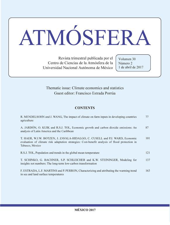
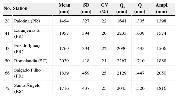
Groups were generated for each homogeneous region. For example, group I was generated based on multivariate analysis, including four rainfall series; group II included nine series; group III, 12 series; group IV, 19 series; group V, 12 series; and finally group VI, 10 series. A chart was then created for each group with the mean values of these series. These charts are shown in Figures 18-23, which allowed the analysis of rainfall variability for each homogeneous region. Tables II-VI show significant meteorological parameters for specific stations in the generated groups.


Mean precipitation, standard deviation, variation coefficient, upper and lower quartiles, and amplitude, for specific stations in group I.
| No. | Station | Mean (mm) | SD (mm) | CV (%) | Qs (mm) | Qi (mm) | Ampl. (mm) |
|---|---|---|---|---|---|---|---|
| 31 | Morretes (PR) | 2155 | 338 | 16 | 2348 | 1973 | 1533 |
| 61 | R. Pequeno (SC) | 2044 | 356 | 17 | 2284 | 1730 | 1227 |
| 62 | T. do Sul (SC) | 1585 | 291 | 18 | 1777 | 1354 | 1247 |
| 75 | T. de Areia (RS) | 1880 | 402 | 21 | 2123 | 1583 | 1857 |
| 77 | P. Grande (SC) | 1848 | 371 | 20 | 2170 | 1527 | 1317 |
SD: standard deviation; VC: variation coefficient; Qs: upper quartile; Qi: lower quartile; Ampl.: amplitude.
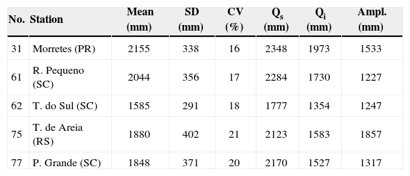
Mean precipitation, standard deviation, variation coefficient, upper and lower quartiles, and amplitude, for specific stations in group II.
| No. | Station | Mean (mm) | SD (mm) | CV (%) | Qs (mm) | Qi (mm) | Ampl. (mm) |
|---|---|---|---|---|---|---|---|
| 25 | Pitanga (PR) | 1781 | 316 | 18 | 2054 | 1579 | 1524 |
| 38 | Lapa (PR) | 1511 | 263 | 17 | 1725 | 1341 | 1102 |
| 45 | Rio Negro (SC) | 1551 | 304 | 19 | 1768 | 1385 | 1317 |
| 54 | A. Carlos (SC) | 1890 | 414 | 21 | 2095 | 1629 | 2415 |
| 57 | Lajes (SC) | 1517 | 300 | 20 | 1693 | 1339 | 1694 |
| 59 | Curitibanos (SC) | 1610 | 350 | 22 | 1850 | 1367 | 1629 |
SD: standard deviation; VC: variation coefficient; Qs: upper quartile; Qi: lower quartile; Ampl.: amplitude.
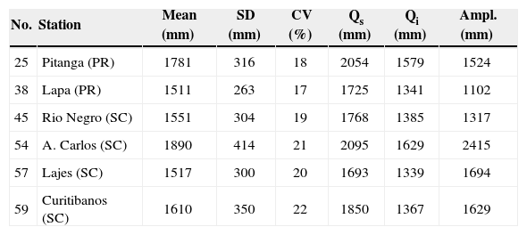
Mean precipitation, standard deviation, variation coefficient, upper and lower quartiles, and amplitude, for specific stations in group III.
| No. | Station | Mean (mm) | SD (mm) | CV (%) | Qs (mm) | Qi (mm) | Ampl. (mm) |
|---|---|---|---|---|---|---|---|
| 46 | U. da Vitória (PR) | 1705 | 390 | 23 | 1862 | 1515 | 1875 |
| 56 | Anitápolis (SC) | 1858 | 318 | 17 | 2049 | 1617 | 1406 |
| 63 | Paim Filho (RS) | 1789 | 339 | 19 | 2009 | 1474 | 1339 |
| 65 | Constantina (RS) | 1784 | 378 | 21 | 2066 | 1569 | 1612 |
| 69 | G. das Missões (RS) | 1488 | 312 | 21 | 1680 | 1251 | 1247 |
SD: standard deviation; VC: variation coefficient; Qs: upper quartile; Qi: lower quartile; Ampl.: amplitude.
Mean precipitation, standard deviation, variation coefficient, upper and lower quartiles, and amplitude, for specific stations in group I V.
| No. | Station | Mean (mm) | SD (mm) | CV (%) | Qs (mm) | Qi (mm) | Ampl. (mm) |
|---|---|---|---|---|---|---|---|
| 28 | Palotina (PR) | 1494 | 327 | 22 | 1641 | 1305 | 1398 |
| 41 | Laranjeiras S. (PR) | 1957 | 394 | 20 | 2233 | 1639 | 1574 |
| 43 | Foz do Iguaçu (PR) | 1769 | 394 | 22 | 2090 | 1495 | 1506 |
| 50 | Romelandia (SC) | 2029 | 418 | 21 | 2267 | 1710 | 1888 |
| 66 | Salgado Filho (PR) | 1839 | 459 | 25 | 2129 | 1447 | 2050 |
| 72 | Santo Ângelo (RS) | 1716 | 437 | 25 | 2045 | 1520 | 1816 |
SD: standard deviation; VC: variation coefficient; Qs: upper quartile; Qi: lower quartile; Ampl.: amplitude.
Mean precipitation, standard deviation, variation coefficient, upper and lower quartiles, and amplitude, for specific stations in group V.
| No. | Station | Mean (mm) | SD (mm) | CV (%) | Qs (mm) | Qi (mm) | Ampl. (mm) |
|---|---|---|---|---|---|---|---|
| 76 | Veranópolis (RS) | 1471 | 229 | 16 | 1615 | 1306 | 970 |
| 80 | Jaguari (RS) | 1820 | 434 | 24 | 2000 | 1482 | 1818 |
| 82 | Tapes (RS) | 1609 | 298 | 19 | 1855 | 1365 | 1104 |
| 83 | Itaqui (RS) | 1635 | 384 | 24 | 1876 | 1389 | 1447 |
| 86 | Sta do Livramento (RS) | 1456 | 360 | 25 | 1692 | 1204 | 1659 |
| 93 | Rio Grande (RS) | 1371 | 319 | 23 | 1591 | 1172 | 1313 |
SD: standard deviation; VC: variation coefficient; Qs: upper quartile; Qi: lower quartile; Ampl.: amplitude.
Group II included part of the states of Paraná and Santa Catarina, presenting coherence with the rainfall regime in this region, with marked annual wave according to the transition of these two states in relation to Rio Grande do Sul, and with homogeneous rainfall regime along the months.
Group IV included the rainfall series of the western regions in the three states. The relative variability of this region is higher than 20%.
Table VI shows values for group V, basically formed by a great part of Rio Grande do Sul, with rainfall values between 1370 and 1820mm. Its relative variability is between 16 and 25%, but the structure of its monthly rainfall distribution has a homogeneous pattern, i.e. without marked variability from month to month.
In general, multivariate analysis created homogeneous subregions inside each region, preserving the rainfall characteristics of the larger areas.
Figures 18 to 23 illustrate the temporal evolution of anomalies for each group. In group I, the year 1983 showed an anomaly of 800mm (i.e. rainfall was 800mm higher than the climatological average). This group consisted of two homogeneous coastal areas in the states of Paraná and Santa Catarina. The year 2003 also showed a marked anomaly (approximately 600mm), whereas 1978, 1979 and 1985 presented negative anomalies (approximately –400mm). The period 1988-1992 showed negative anomalies, i.e. rainfall values were lower than the climatological average in this homogeneous area, with year 1989 presenting the lowest irregular values (below –400mm). In 2003 precipitation was also below the climatological average. In 14 of the 35 years analyzed rainfall was below the climatological average, whereas 16 years showed values above the average.
For the same temporal evolution of group II, the values of anomalies were significant but not as pronounced as in group I (Fig. 19). This homogeneous area involves the mid-eastern region of the states of Paraná and Santa Catarina. Rainfalls in 1983 and 1998 were above the climatological average (600mm). Variability in the rainfall pattern from one area to another was detected. In 1985, the anomaly was approximately –600mm, characterizing it as a drier year in this homogeneous area, compared with group I, previously analyzed. In this group, 12 years with negative anomalies and 13 years with positive anomalies were recorded in the study area.
The temporal evolution of anomalies for the homogeneous regions of groups III and IV are shown in Figures 20and 21. The difference of rainfall values for these two groups compared to preceding groups is remarkable. Group III presented rainfall values well above the average in 1983 (1000mm above the climatological average) and 1998, with anomaly greater than 800mm. Negative anomalies were also significant in this area. In 1978, 1985, 1991 and 2006, negative anomalies were lower than –600mm. This group is located at the mid part of the southern region, with areas of Paraná, Santa Catarina and northern state of Rio Grande do Sul. Positive anomalies occurred in nine years, and negative anomalies occurred in 13 years (Fig. 20). In this group, precipitation was above the average in 17 years and below the average in 14 years.
The homogeneous area corresponding to group IV is located to the west of the states of Paraná, Santa Catarina and Rio Grande do Sul (Fig. 21). This group presented anomalies with values lower than other groups. For example, the years 1983, 1997, 1998 and 2002 presented positive anomalies above 400mm and below 600mm. Marked negative anomalies occurred in 1978, 1985, 1988, 1999, 2006 and 2007. In group IV, rainfall value was above the average in 14 years and below the average in 17 years, within the study period.
Figures 22and 23 show anomalies for the homogeneous regions corresponding to groups V and VI, respectively. Group V corresponds to practically the entire state of Rio Grande do Sul, i.e. the southernmost part of the southern region, and presented a marked anomaly in 2002, 800mm higher than in 1982-1983 and 1997-1998 ENSO events (warm phase), considered the most intense events in the last three decades. The northern and northwestern state of Paraná, corresponding to group VI, presented values of anomalies below 600mm, highlighting 1980 and 2006, with values greater than 400mm of positive anomalies.
It is worth mentioning the negative anomaly in 1982 (–400mm) in this homogeneous classified area. In group V precipitation values were above the climatological average in 14 years and below the average in 17 years. For group VI, 11 years within the study period presented rainfall above the average, and 10 years below the average.
4ConclusionThe filling of gaps and the homogenization carried out based on the R environment and Climatol subroutine is satisfactory, generating a more reliable database to perform statistical inferences, allowing a better ordination of data used.
There was a marked rainfall variability in southern Brazil, and part of the states of Paraná and Santa Catarina had a well-marked annual wave, with maximum in the summer and minimum in the winter. In other areas, the rainfall structure was distinct, with rainfall distributed over the year.
The precipitation value was analyzed for some years, and spatial and temporal (annual) variability was detected. In general, the southern region had rainfall above the climatological average during El Niño years. Also, not all ENSO events (warm phase, El Niño) produce the same rainfall response for this region.
Anomalies also presented a marked variability from year to year. In 1976, values of anomalies were low, i.e. rainfall was not far above the average. In 1982, there were anomalies above 100mm, i.e. 100mm above the climatological average. In 1983 (considered a year of intense El Niño), the Southern region presented markedly positive anomalies in almost the entire study area.
In 1982, positive anomalies were verified, with rainfall above the average: 400mm in the northwestern state of Rio Grande do Sul. In the next year (1983), the anomaly was even more positive, with values above 1000mm (i.e., 1000mm above the average).
In 1985, negative anomalies were observed in great part of the southern region, with values of –600mm in the mid part of the state of Paraná.
Precipitation was also evidently higher than the average in this region, with anomaly values exceeding 900mm in the western region of the states of Paraná and Santa Catarina.