

Por primera vez se presentan mapas de concentración superficial de dióxido de nitrógeno (NO2) para el territorio colombiano. Se infirieron concentraciones superficiales de NO2 para 2007 a partir de dos fuentes de datos de densidad de columna troposférica: 1) una simulación que utiliza el modelo global tridimensional GEOS-Chem y 2) mediciones realizadas por el instrumento de monitoreo del ozono (OMI, por sus siglas en inglés) instalado a bordo del satélite Aura de la NASA. Los resultados muestran valores mensuales promedio de 0.1 a 6 ppbv. Se compararon las concentraciones superficiales de NO2 inferidas con mediciones in situ corregidas y se encontraron coeficientes de correlación de hasta 0.91. Una fuente importante de NO2 es la quema de biomasa, la cual puede ser diagnosticada a partir de los datos de potencia radiativa de los fuegos provenientes del reanálisis para el monitoreo de la composición atmosférica y el clima (MACC, por sus siglas en ingés). Se encontró una fuerte relación entre altas concentraciones de NO2 inferidas y quema de biomasa para un área extensa que comprende los departamentos de Caquetá, Meta, Guaviare, Vichada y Putumayo.
For the first time, maps of surface concentration of nitrogen dioxide (NO2) are presented for the Colombian territory. NO2 surface concentrations for the year 2007 are inferred based on two sources of tropospheric NO2 column data: (1) a simulation using a three-dimensional global model (GEOS-Chem) and (2) measurements made by the ozone monitoring instrument (OMI) onboard the NASA Aura satellite. Results show monthly averages between 0.1 and 6 ppbv. We compare these inferred values to corrected ground measurements of NO2. We find correlation coefficients of up to 0.91 between the inferred data and the corrected observational data. A significant source of NO2 is biomass burning, which can be diagnosed by data of fire radiative power (FRP) from the Monitoring of Atmospheric Composition and Climate (MACC) reanalysis. We find a close relationship between high values of inferred NO2 surface concentrations and biomass burning for a large area which encompasses the departments of Caquetá, Meta, Guaviare, Vichada, and Putumayo.
NO2 is both an important contributor to ozone (O3) decomposition in the stratosphere and a major precursor in the chain of chemical reactions that produces O3 in the troposphere. Both O3 and NO2 are toxic to biota. Long-term exposure to NO2 is significantly associated with decreased lung function and is a risk factor for respiratory diseases (Ackermann-Liebrich, 1997; Schindler et al., 1998; Gauderman, 2000, 2002; Panella et al., 2000; Smith et al., 2000). The measurement of pollutants not only allows the tracking of anthropogenic activity, but also improves our understanding of the relationships between pollution and natural phenomena. In this study, we focus on NO2. Nitrogen oxide (NO) and NO2 species are produced from lightning, biomass burning, fossil fuel combustion, and soils (Sauvage et al., 2007). The high temperatures of combustion break down molecular oxygen (O2) from the air, which subsequently enters an important chemical reaction that produces NO and NO2 (Jacob, 1999). Their production in combustion makes NOx a marker of industrial activity (including fossil fuel-based power generation, transportation, and concrete manufacture) as well as other human activities, such as agricultural biomass burning. Therefore, NO2 serves as an indicator of air quality and anthropogenic activity. Researchers have made significant efforts to analyze pollutant emission and overall air quality in Colombia, but none were focused specifically on NO2 (Lacouture, 1979; Bedoya, 1981; Ruiz, 2002; Benavides, 2003; Barreto, 2004; Jiménez, 2004; Oviedo, 2009).
Our primary interest in this study is the inference of surface NO2 concentrations in Colombia. To infer these concentrations, we use the GEOS-Chem tro-pospheric chemistry model along with tropospheric column data from the ozone-measuring instrument (OMI) onboard the NASA Aura satellite. The first step of the inference process was the acquisition of NO2 tropospheric column data from the OMI. We use the OMNO2e product (Kempler, 2010). There are other OMI products that report NO2 density of tropospheric columns, such as the different products of the Royal Netherlands Meteorological Institute (KNMI) (Boersma et al., 2007, 2011). However, the analysis of these products and their intercomparison are beyond the scope of this study.
Aerial measurements reveal that the concentration of NO2 in the tropospheric column is determined primarily by NO2 in the mixed layer, as well as by that in the boundary layer (Martin et al., 2004, 2006; Boersma et al., 2008; Bucsela et al., 2008). However, the proportion of NO2 in these two layers varies in space and time. Lamsal et al. (2008) proposed a method that uses the local NO2 profiles obtained from the GEOS-Chem model to capture this variation in space and time. The GEOS-Chem model is a global three-dimensional model of tropospheric chemistry driven by assimilated meteorological observations from the Goddard Earth Observing System (GEOS) of the NASA Data Assimilation Office (Bey et al., 2001; Gass, 2012; Rienecker et al., 2008). This model provides a comprehensive description of atmospheric composition and allows us to obtain tropospheric column densities and profiles up to 0.01 hPa. These profiles are used together with the tropospheric column data from OMI (see details in section 4.5) to infer quasi-observed concentrations of NO2 at the surface.
Celarier et al. (2008) validated the tropospheric, stratospheric and total NO2 columns from the OMI with respect to surface measurements from multiple sources. This validation is difficult for many reasons, perhaps the most important of which is that each OMI column corresponds to the average over a large area (at least 340 km2), whereas surface measurements are site-specific. In addition, surface measurement instruments are often placed at points of maximum emission and, therefore, do not measure background concentrations. Another difficulity is that the length of each time data series for validation is short, and the number of series is small, which makes statistical analysis difficult. Despite these and other difficulties, OMI measurements and surface measurements yield correlations in the data that are generally above 0.6. Another way to validate the tropospheric columns is through air campaigns or in situ experiments, which provide vertical profile data. Boersma et al. (2008) reported a high similarity between OMI data and in situ profile data.
For the first time, maps of surface concentration of NO2 are presented for the Colombian territory for a whole year, 2007. Additionally, in order to assess the contribution of the biomass burning to the NO2 concentrations in the country, the inferred surface NO2 concentrations are compared with fire radiative power data, which is used to monitor biomass burning. A brief summary of all the datasets used is given in section 2. Section 3 describes the methods used to infer the surface concentrations of NO2 and to calculate the correction factors to NO2 concentrations measured at surface stations. The results and conclusions are presented in sections 4 and 5.
2Data2.1NO2 tropospheric column from OMIWe used data from the OMNO2e product, which is a daily, global, gridded data product, where each file is produced from one day’s worth of NO2 measurements made by the ozone monitoring instrument onboard the EOS-Aura spacecraft (OMI Team, 2009). The data are filled into a grid with horizontal resolution of 0.25 × 0.25º in latitude and longitude. The data fields included in the product are two: (a) total column NO2 in units of molecules/cm2, cloud-screened at 30%; and (b) tropospheric column NO2, cloud-screened at 30%. For each grid cell a field-of-view (FOV) weighted estimate was calculated for each field (Bucsela et al., 2006; Kempler, 2010). The Aura satellite passes over Colombian territory at 17:00 and 18:00 UTC or 12:00 and 13:00 LT.
The reported NO2 column corresponds to the visible range (between 405 and 465 nm), i.e., in the presence of clouds, the amount of NO2 reported corresponds to the amount found above these. The maximum detection limit for a cloudy area is 30%, meaning that when cloud cover is below this value, there should be no bias in the data calculated using the standard algorithm (Torres et al., 2002). For grid cells with cloud covers above 30%, both total and tropospheric NO2 columns are set to missing values.
2.2GEOS-Chem simulationTo infer the NO2 concentrations at the surface, information about the NO2 tropospheric profile is required. To obtain this profile, we used the GEOS-Chem 3D global tropospheric chemistry model. The GEOS-Chem simulation performed is of the type “NOx-Ox-hy-drocarbons” and has a spatial resolution of 2.5 × 2º. GEOS-Chem simulates tropospheric ozone-nitrogen oxides-hydrocarbon chemistry. We used version v8-02-01, in which there are 43 advected tracers. The simulation with GEOS-Chem was performed for 47 vertical levels that ranged from the surface to 0.01 hPa, and covers the years 2006 and 2007. The year 2006 served as a model spin-up. The simulation includes the reaction mechanisms SMVGEAR II and FAST-J for photolysis (Evans et al., 2003).
Although there are emissions inventories for some cities, there is no national emission inventory available for Colombia. For this reason, we used the default inventories suggested by the GEOS-Chem team according to the region of the world (see Table 2 in http://acmg.seas.harvard.edu/geos/word_pdf_docs/emissions_v8_02_03.pdf). In particular for Central and South America, the NOx, SOx and CO emissions are from EDGAR 3.2 FT (Olivier and Berdowski, 2001); the VOC and NH3 emissions are from GEIA (Wang et al., 1998); and BC/OC emissions are from Bond et al. (2007). Emissions from open fres for individual years were taken from the monthly GFED2 inventory (van der Werf et al., 2009). The emissions are available from 1997 to 2008 (see item 4.2.16 in http://acmg.seas.harvard.edu/geos/doc/man/chapter_4.html), so the fires occurring in 2007 are included in the model on a monthly basis.
2.3Surface data from air quality stationsTo validate the inferred surface concentrations, we used NO2 data from stations of the air quality monitoring networks installed in Bogotá and Bucar-amanga (Fig. 1) by the Secretaría Distrital de Ambiente (District Department of Environment) and the Corporación Autónoma Regional para la Defensa de la Meseta de Bucaramanga (Regional Autonomous Corporation for the Defense of the Bucaramanga Plateau), respectively. For Bogotá, we used data from seven stations: IDRD, MAVDT, Fontibón, Las Ferias, Suba, Puente Aranda, and Carvajal. For Bucaramanga, we used data from the Centro station. These data represent measurements made using commercial chemiluminescence equipment.
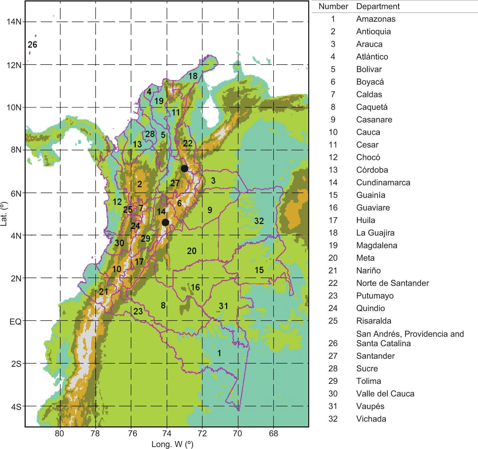
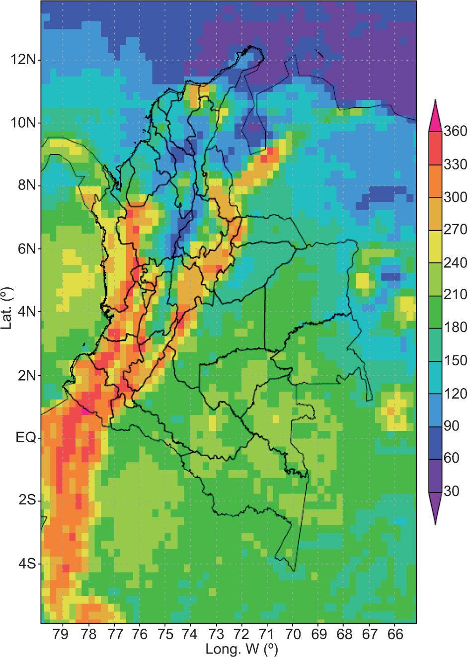
. Beyond the Colombian Massif (in the south-western departments of Nariño and Cauca) the Andes are divided into three branches known as cordilleras (mountain ranges): the Cordillera Occidental (West Andes), the Cordillera Central (Central Andes), and the Cordillera Oriental (East Andes).")
Political map and topography of Colombia. For this study, in situ measurements were available only from those stations indicated by black circles (Bogotá and Bucaramanga). Beyond the Colombian Massif (in the south-western departments of Nariño and Cauca) the Andes are divided into three branches known as cordilleras (mountain ranges): the Cordillera Occidental (West Andes), the Cordillera Central (Central Andes), and the Cordillera Oriental (East Andes).
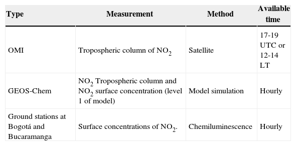
All of the NO2 data used in this study represent values measured between 17:00 and 19:00 UTC. The period of greatest coverage of the Colombian territory by the Aura satellite is between 17:00 and 19:00 UTC (12:00 and 14:00 LT). For this reason, the NO2 data obtained from each source (in situ, OMI and GEOS-Chem) were averaged for these two hours. Subsequently, monthly averages for each NO2 data-set were calculated using these values only at those days when OMI data are available. Table I shows an overview of the data used in this work.
Overview of the NO2 data used.
| Type | Measurement | Method | Available time |
|---|---|---|---|
| OMI | Tropospheric column of NO2 | Satellite | 17-19 UTC or 12-14 LT |
| GEOS-Chem | NO2 Tropospheric column and NO2 surface concentration (level 1 of model) | Model simulation | Hourly |
| Ground stations at Bogotá and Bucaramanga | Surface concentrations of NO2. | Chemiluminescence | Hourly |
Lamsal et al. (2008) proposed a method that uses the local NO2 profile obtained from the GEOS-Chem model to capture the variation in space and time of the NO2 concentration. Based on the GEOS-Chem profiles, the OMI concentrations at the surface can be estimated as follows:

In this equation, S represents the superficial level concentration, and represents the NO2 tropospheric column. The subindex O indicates OMI, and the subindex G indicates GEOS-Chem. The OMI-derived surface concentration So represents the mixing ratio in the lowest layer of the model, which is approximately 70 m (Le Sager et al, 2008).
The spatial variation of the OMI observations (which have an original resolution of 0.25 × 0.25º) within the resolution of the GEOS-Chem simulation (2.5 × 2º) should reflect variation in NO2 concentrations within the boundary layer. Lamsal et al. (2008) developed a scheme to combine both sources of information (vertical profile and horizontal variation) to infer concentrations of NO2 at the OMI resolution, as follows:
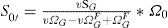
In Eq. (2), So′ is the surface level NO2 concentration, í is ass factor that describes the influence of the lower levels of the troposphere in the mixture of NO2, and ΩGF corresponds to the free tropospheric column, which is taken as a horizontal constant on the GEOS-Chem grid and refects the longest NO2 half-life in the free troposphere. The calculation of ΩGF determines the planetary boundary layer and calculates the existing column at and above this layer. v is given by:

In this equation, Ω0 corresponds to the NO2 tropospheric columns from the OMI (0.25 × 0.25º), and Ω0¯ corresponds to the OMI tropospheric columns averaged at the GEOS-Chem grid resolution (2.5 × 2.0º). Eq. (2) becomes Eq. (1) when í is equivalent to unity.
3.2Interference in the measurement of NO2Once the surface concentrations of NO2 are inferred, it is necessary to validate these concentrations. The NO2 measuring instrument most commonly used by air quality monitoring networks globally is the che-miluminescence analyzer, which contains a catalytic molybdenum converter (Ellis, 1975). This instrument is subject to significant interference from other oxidized substances, such as peroxyacytyl nitrate (PAN), nitric acid (HNO3), and organic nitrates (Grosjean and Harrison, 1985; Dunlea et al, 2007; Steinbacher et al, 2007). To correct this interference at the surface, correction factors (CF) were calculated using the GEOS-Chem model. Fig. 1 shows the location of the stations, from which in situ measurements were available for this study.
Commercial chemiluminescence detectors are powered by the intensity of light produced by the chemical reaction between ozone (provided by the measuring instrument) and NO, as follows:
In this reaction, NO2* corresponds to an excited NO2 molecule, which will subsequently lose a measurable amount of energy. This process involves the chemical reduction of NO and the use of a molybdenum catalytic converter heated to 300-400 °C to catalyze the chemiluminescence reaction described above. The instrument has two modes of measurement: NO and NOx. The concentration of NO2 is determined by subtracting the two reading modes (NOx-NO). The disadvantage of this approach is that not only NO2 is chemically reduced; other species, such as HNO3, PAN, and alkyl nitrate (AN), can also contribute. We used the CF developed by Lamsal et al. (2008) to correct our estimate of the concentration of surface NO2:
4Results4.1NO2 columns from the GEOS-Chem model
Figure 2 shows the monthly mean density of tropospheric NO2 columns obtained from the GEOS-Chem model simulation for Colombia. To calculate the monthly means, the model data was sampled only at those times when OMI data is available. The density of the tropospheric columns is relatively low, with values not exceeding 1.0 × 10¹⁵ molecules/cm2. The column density varies by region. Lower values (≈ 0.2 × 10¹⁵ molecules/cm2) are observed in southern and southeastern Colombia in departments that contain notable rainforest areas, including Amazonas, Caquetá, Putumayo, Vaupés, Guaviare, and Guainía. Slightly higher tropospheric column values (> 0.4 × 10¹⁵ molecules/cm2) are observed in northern Colombia in such departments as Córdoba, Sucre, Bolívar, Atlántico, Magdalena, Cesar, and La Guajira (as well as in Venezuela). Figure 2 also shows that in some cases, consecutive months have similar tropospheric NO2 column averages.
![Monthly average densities (in molecules/cm2 [× 1015]) of tropospheric NO2 columns from the GEOS-Chem model. Only the maps for even months are shown. For the calculation of the monthly averages, each grid cell of the density data (available in a resolution of 2.5 × 2.0º) was divided into 80 grid boxes of equal size (0.25 × 0.25º). Additionally, the GEOS-Chem density data was sampled only at those times when OMI data is available. Blank (white) grid boxes represent missing OMI data.](https://static.elsevier.es/multimedia/01876236/0000002700000002/v2_201505081734/S0187623614711105/v2_201505081734/en/main.assets/gr2.jpeg?xkr=ue/ImdikoIMrsJoerZ+w997EogCnBdOOD93cPFbanNd17ZbJhz9Sq061KafGNBfGkoHH/COD/yuxMMO/xDWDHvncbZRy8EKCI+jhWLymvNAz9y58zTSGNieFfhtisnqvYFzMxkd5UhV9UQU83Fz2HnBF+PnT3hnL55D+mJJnstsDl7ijOy6DZ8gxhK5Pi1HOh6kQleaty+eFqXocKtXFx6pOPRFaTEMFb5c0h8z1VftmIjXwjxIYiR34SZCep3Myj8jBKy2K3m8QxlEQYSMbR+y3wsKa5Kj6t0NhY5zUmlY= "Monthly average densities (in molecules/cm2 [× 1015]) of tropospheric NO2 columns from the GEOS-Chem model. Only the maps for even months are shown. For the calculation of the monthly averages, each grid cell of the density data (available in a resolution of 2.5 × 2.0º) was divided into 80 grid boxes of equal size (0.25 × 0.25º). Additionally, the GEOS-Chem density data was sampled only at those times when OMI data is available. Blank (white) grid boxes represent missing OMI data.")
Monthly average densities (in molecules/cm2 [× 1015]) of tropospheric NO2 columns from the GEOS-Chem model. Only the maps for even months are shown. For the calculation of the monthly averages, each grid cell of the density data (available in a resolution of 2.5 × 2.0º) was divided into 80 grid boxes of equal size (0.25 × 0.25º). Additionally, the GEOS-Chem density data was sampled only at those times when OMI data is available. Blank (white) grid boxes represent missing OMI data.
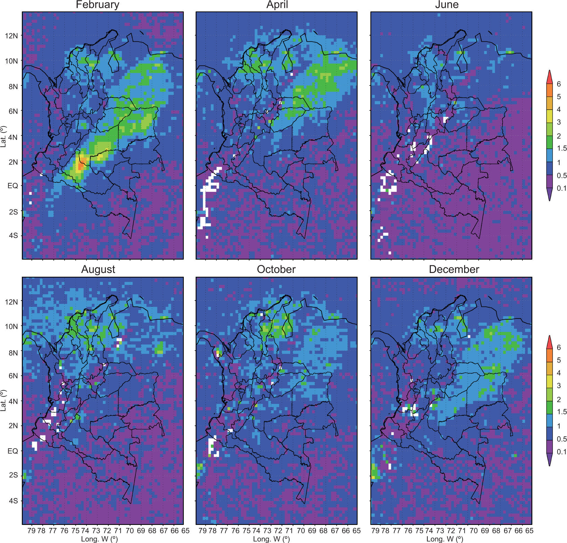
The surface level NO2 concentrations from the GEOS-Chem model are presented in Figure 3. Relatively low NO2 surface concentration values were obtained over most of Colombia. Lower values were observed in the southern, southeastern and Pacific regions, where anthropogenic activity is low or nonexistent, and slightly higher values (up to 0.5 ppbv) were observed to the north along the Caribbean coast into Venezuela, where population density, agriculture, and industrial and mining activities are the greatest. This pattern is similar to that observed in the tropospheric column data from GEOS-Chem, which reflects the expected distribution of pollutants, as in forested areas or areas with little population, the surface concentration of NO2 should be low compared to that observed in more populated areas or in areas of agricultural or industrial activities. This suggests a strong influence of the lower layers on the general properties of the tropospheric NO2 column, probably because chemically formed NO2 is generated mainly through land use and the burning of both fuels and biomass.
 from the GEOS-Chem model. Same remarks as in Figure 2.")
Monthly averages of NO2 surface concentration (in ppbv) from the GEOS-Chem model. Same remarks as in Figure 2.
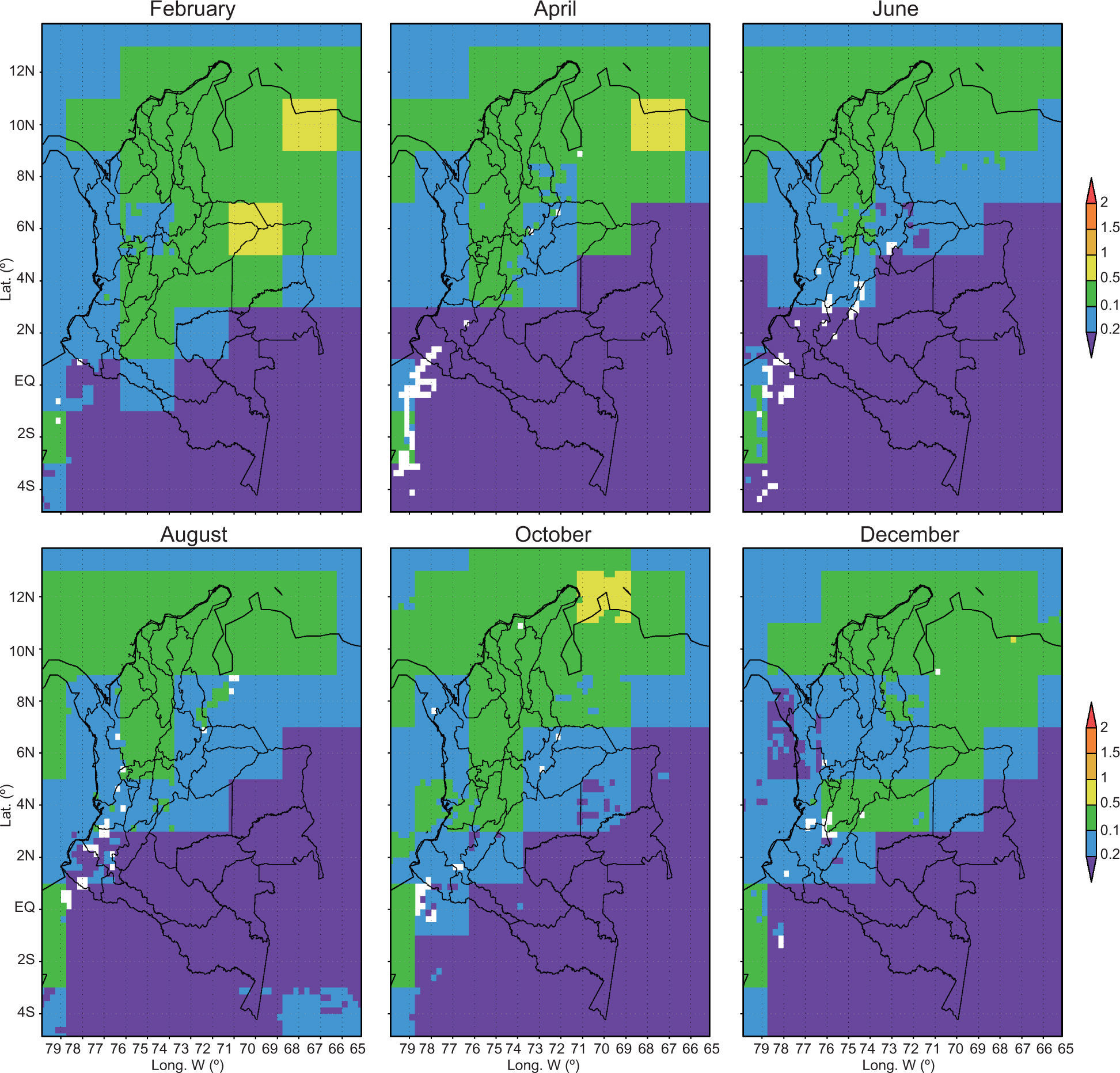
The density values of the tropospheric NO2 columns from the OMI are shown in Figure 4. As was true for the GEOS-Chem data, we can see that in general, for most months, lower values are found in the southern and southeastern areas comprising departments with rainforest areas, including Amazonas, Vaupés, Guainía, Putumayo, Caquetá, and Guaviare. Another area with low concentration values is the Pacific region to the west, which includes departments of Chocó, Valle del Cauca, Cauca, and Nariño. Higher values are found mainly to the north, in departments such as Córdoba, Sucre, Bolívar, Magdalena, Atlántico, and Cesar, as well as in Venezuela. The month with the lowest density values for the whole country is June. On the other hand, high-density values were reported by the OMI in February. In this month, a continuous strip of densities of 2 × 10¹⁵ molecules/ cm2 or greater is observed between western Venezuela and the departments of Vichada, Arauca, Casanare, Meta, and Caquetá, which are not densely populated. However, oil extraction is the main economic activity in the last four departments and in western Venezuela. The strip occurs in January (and also in December), covering western Venezuela and the departments of Vichada, Arauca, and Casanare, then reaches a maximum in February and declines approximately in April. At its peak, this continuous strip of high concentrations extends to the southwest and eastward to Caquetá, Putumayo, and Guaviare. These relatively high concentrations of NO2 may be associated with such factors as biomass burning, improper agricultural soil management, burning associated with the oil industry or the transport of NO2 from other regions.
4.4Comparison of GEOS-Chem columns and OMI columns![Monthly average densities of tropospheric NO2 columns (in molecules/cm2 [× 1015]) from the OMI for 2007. Grid resolution is 0.25 × 0.25º. Blank (white) grid boxes represent missing data. Only the maps for even months are shown.](https://static.elsevier.es/multimedia/01876236/0000002700000002/v2_201505081734/S0187623614711105/v2_201505081734/en/main.assets/gr4.jpeg?xkr=ue/ImdikoIMrsJoerZ+w997EogCnBdOOD93cPFbanNd17ZbJhz9Sq061KafGNBfGkoHH/COD/yuxMMO/xDWDHvncbZRy8EKCI+jhWLymvNAz9y58zTSGNieFfhtisnqvYFzMxkd5UhV9UQU83Fz2HnBF+PnT3hnL55D+mJJnstsDl7ijOy6DZ8gxhK5Pi1HOh6kQleaty+eFqXocKtXFx6pOPRFaTEMFb5c0h8z1VftmIjXwjxIYiR34SZCep3Myj8jBKy2K3m8QxlEQYSMbR+y3wsKa5Kj6t0NhY5zUmlY= "Monthly average densities of tropospheric NO2 columns (in molecules/cm2 [× 1015]) from the OMI for 2007. Grid resolution is 0.25 × 0.25º. Blank (white) grid boxes represent missing data. Only the maps for even months are shown.")
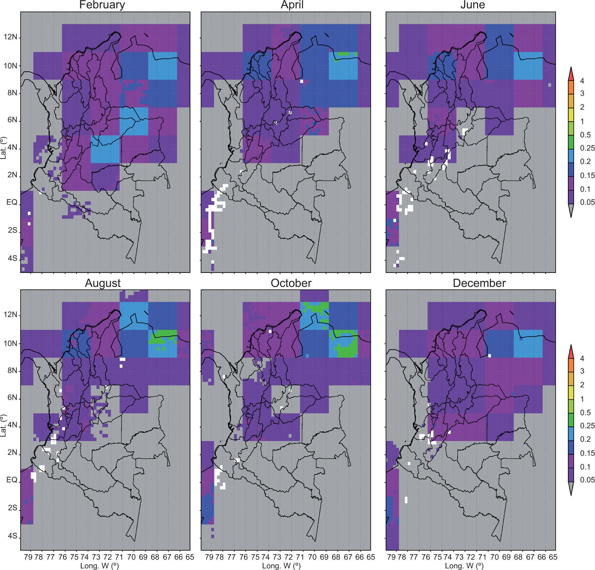
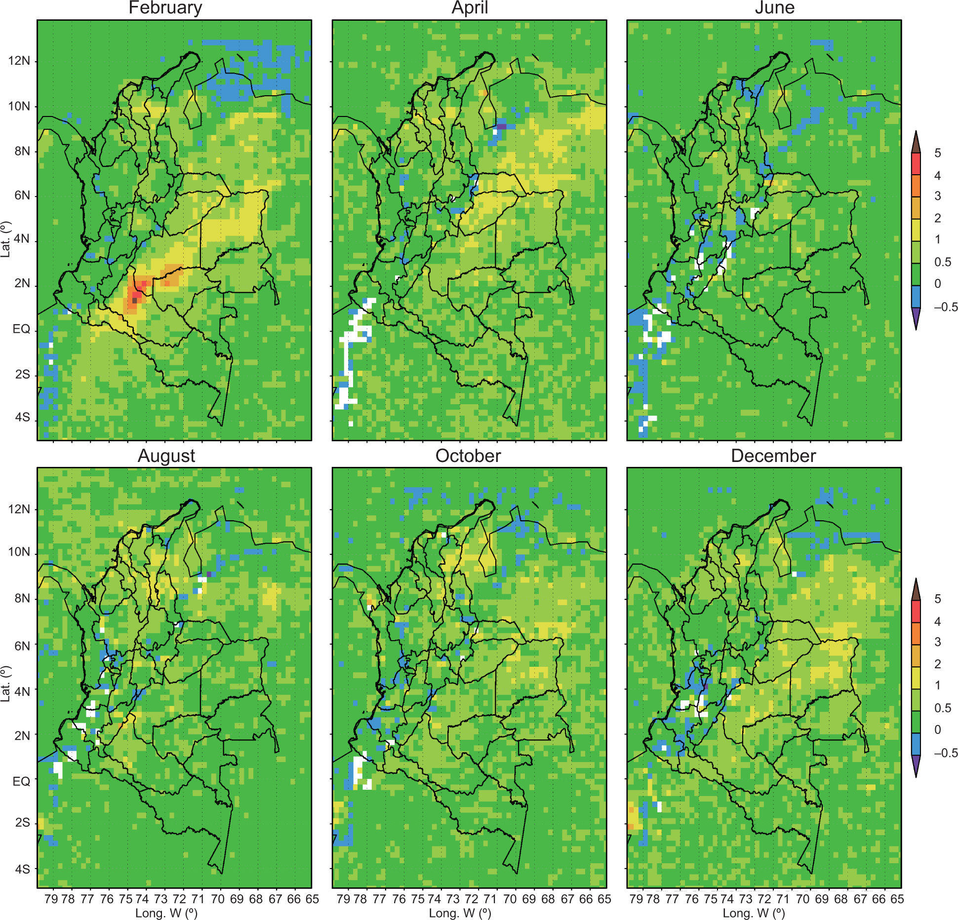
Figure 5 shows the result of subtracting monthly OMI column densities from GEOS-Chem column densities (Figs. 4 and 2, respectively). To perform this subtraction, each grid cell of the GEOS-Chem data, available in a resolution of 2º × 2.0º, was divided into 80 grid cells of equal size (0.25 × 0.25º). Additionally, the GEOS-Chem data was sampled only at those times when OMI data is available. In general, tropospheric column densities from OMI are systematically higher than those from GEOS-Chem. However, there are spots where column densities from OMI are lower than those from GEOS-Chem. These spots are mountain areas located on the Cordillera Oriental, Cordillera Occidental, Ecuadorian Andes, and Venezuelan Andes. There are also some spots located to the north, in the departments Guajira, Cesar, and Magdalena.
![Mean differences between OMI and GEOS-Chem monthly tropospheric NO2 columns (in molecules/cm2 [× 1015]). Only the maps for even months are shown.](https://static.elsevier.es/multimedia/01876236/0000002700000002/v2_201505081734/S0187623614711105/v2_201505081734/en/main.assets/gr5.jpeg?xkr=ue/ImdikoIMrsJoerZ+w997EogCnBdOOD93cPFbanNd17ZbJhz9Sq061KafGNBfGkoHH/COD/yuxMMO/xDWDHvncbZRy8EKCI+jhWLymvNAz9y58zTSGNieFfhtisnqvYFzMxkd5UhV9UQU83Fz2HnBF+PnT3hnL55D+mJJnstsDl7ijOy6DZ8gxhK5Pi1HOh6kQleaty+eFqXocKtXFx6pOPRFaTEMFb5c0h8z1VftmIjXwjxIYiR34SZCep3Myj8jBKy2K3m8QxlEQYSMbR+y3wsKa5Kj6t0NhY5zUmlY= "Mean differences between OMI and GEOS-Chem monthly tropospheric NO2 columns (in molecules/cm2 [× 1015]). Only the maps for even months are shown.")
In Colombian remote regions, industrial activity is very little and volcanic activity is scarce. When there is not biomass burning in these regions, NO2 columns are determined by both lightning production and transport of pollutants from other regions. Therefore, density of tropospheric NO2 columns over these regions should have values close to zero. That should occur in departments of Amazonas and Vaupés and in parts of the departments of Guanía, Vichada, Caquetá, and Guaviare. In these regions, OMI (GEOS-Chem) columns have density values between 0.4 and 1.5 (0 and 0.8) × 1015 molecules/cm2 (see Figs. 2 and 5). Thus, there is overestimation of OMI columns in remote regions.
Validation of satellite observations of tropospheric NO2 columns has been carried out in non-remote regions by both using differential optical absorption spectroscopy (Celarier et al., 2008) and by performing aircraft measurements over the US and Mexico (Boersma et al., 2008). These authors reported that correlations between in situ NO2 measurements and satellite observations in some remote areas are not greater than 0.6.
To quantify the overestimation of NO2 column densities in remote regions by OMI, a bias correction value is calculated as the average of all the monthly differences between OMI and GEOS-Chem column densities for year 2007 and for all the grid points comprised in two rectangular areas: 1.50° N to 0.75° S, 71.50 to 70.00° W, and 0.75 to 2.25° S, 73 to 69.5° W. These two areas comprise the major part of the departments of Vaupés and Amazonas. A bias correction value of 0.4 × 10¹⁵ molecules/cm2 was found. Therefore, we propose that on points where the density of OMI NO2 columns is expected to be very low, this value should be subtracted.
From Eqs. (1) and (2) it can be inferred that if the tropospheric column density in a given area is overestimated (underestimated) by OMI-derived measurements, our inferred surface concentration is thus also overestimated (underestimated). These biases can be caused by the derivation of the OMI tropospheric column, since the stratospheric contribution has to be estimated and subtracted.
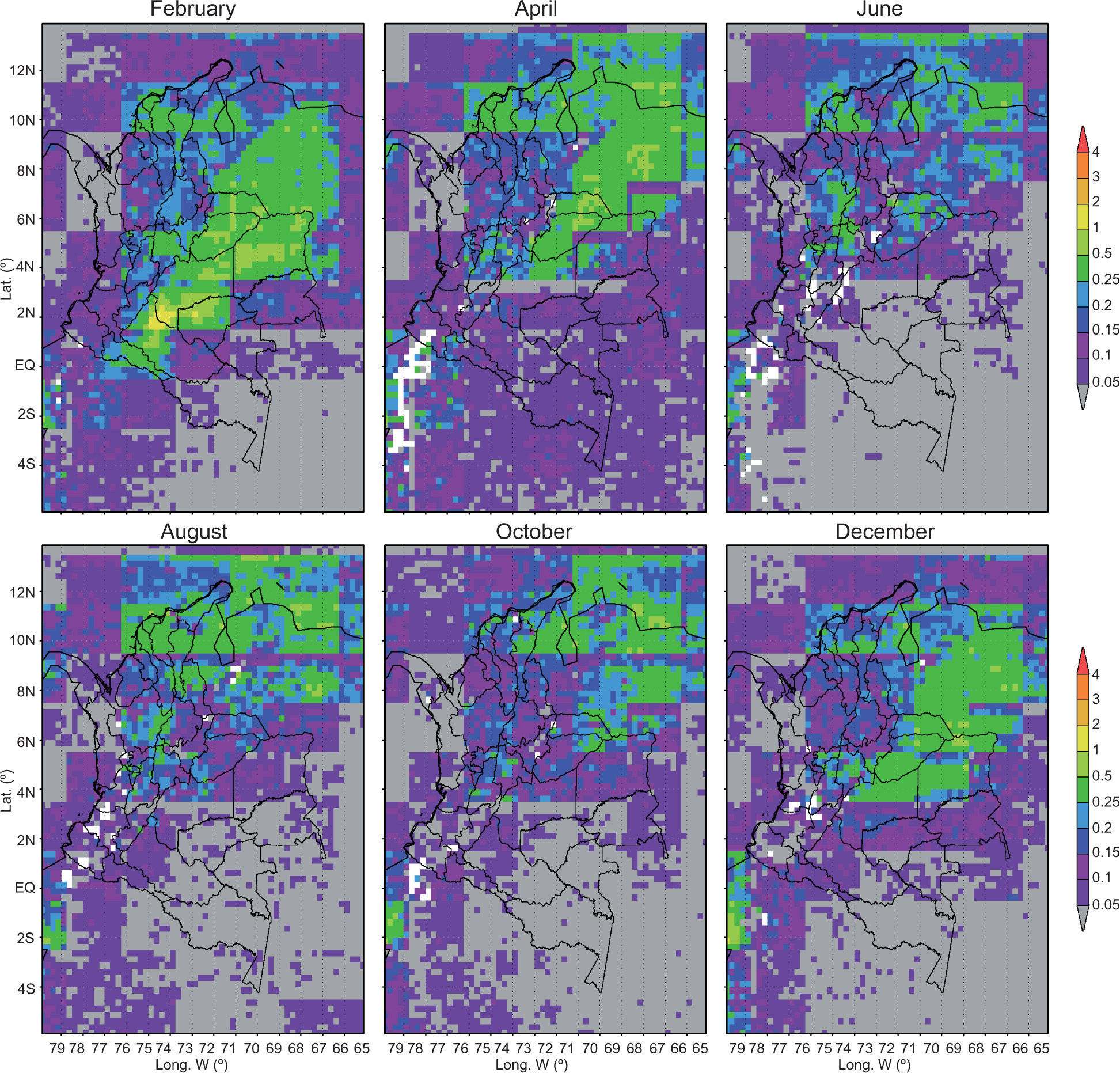
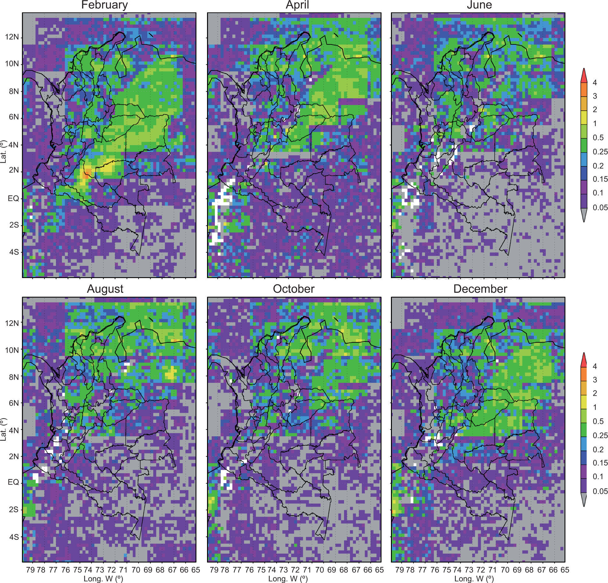
4.5Inference of surface NO2 concentrationsSurface concentrations of NO2 were inferred by using Eqs. (1) and (2). These inferred concentrations are presented in Figures 6 and 7. Figure 6 shows the results based on Eq. (1), and Figure 7 shows those based on Eq. (2). For the construction of both figures, it was necessary to perform a conservative remapping (Jones, 1999) of the GEOS-Chem tropospheric columns and the GEOS-Chem surface concentrations to the 0.25 × 0.25º OMI grid in order to carry out the numerical calculations involved in Eqs. (1) and (2). Eq. (2) generated higher surface concentration values than Eq. (1). This result is due to the greater influence of the lower layers of the troposphere implied in the method of calculation used by Eq. (2). This equation includes two fundamental aspects. The first is the influence in the horizontal plane of the factors v on the tropospheric columns (G and ΩGF) and the surface concentrations from the model (SG), which influence results in a larger NOx lifetime in the free troposphere. Factors ν describe the influence of the lower parts of the troposphere on the values of NO2 in the whole column. The 2.5 × 2º grid is affected according to the OMI column values, which have a resolution of 0.25 × 0.25º. The second aspect is the influence in the vertical dimension of the free tropospheric ΩGF columns, which differentiate the tropospheric column into a planetary boundary layer and the rest of the column (which is called the free tropospheric column). The effects of the planetary boundary layer and the even stronger effects of the mixed layer (given the generation of NO2 on the surface) can be observed by comparing Figures 5 and 6, which show that higher surface concentrations of NO2 are obtained using Eq. (2).
 inferred using Eq. (1). Same remarks as in Figure 4.")
 inferred using Eq. (2). Same remarks as in Figure 4.")
Figure 7 highlights the high concentrations of NO2 inferred for the month of February at the boundaries between the departments of Caquetá and Meta and between the departments of Meta and Guaviare. At the boundary between Caquetá and Meta, values of more than 3 ppbv are observed. These values are comparable to those observed in densely populated cities in the United States (Lamsal et al, 2008). Ichoku et al. (2008) found that across a region between 5° N and 5° S, and 75 and 50° W (including parts of Colombia, Venezuela, Perú, Bolivia, Brazil, Guyana, Suriname, and French Guiana), the fire diurnal cycle has combustion rates peaking early in the afternoon (between 12:00 and 15:00 LT). OMI-derived NO2 concentrations are inferred for the period between 12:00 and 14:00 LT, and the high NO2 concentrations in the departments of Caquetá, Meta and Guaviare in February are highly associated with biomass burning (as will be shown in section 4.7.2). Thus, a value of 3 ppbv in the departments of Caquetá, Meta and Guaviare in February would be close to the monthly mean of the daily maximum. For other months, from May to November, when little biomass burning is recorded (section 4.7.2), the inferred OMI NO2 values should correspond to low values in the daily production cycle (due to the relatively high rate of photodissociation of NO2 around noon, which is when the satellite Aura passes over the region [Barreto, 2004]). Thus, NO2 concentrations almost certainly reach higher values in the afternoon and evening when the rate of photodissociation of NO2 is reduced.
4.6Correction of NO2 concentrations measured at surface stationsTo compare the surface NO2 concentrations inferred from OMI data with the in situ data collected at surface stations, it was necessary to correct the latter. As mentioned in section 3.2 above, NO2 concentrations registered using commercial chemiluminescence gauges are higher than the true concentrations because in these measuring devices, NOy species other than NO2 (including the alkyl nitrates, HNO3 and PAN) are subject to chemical reduction.
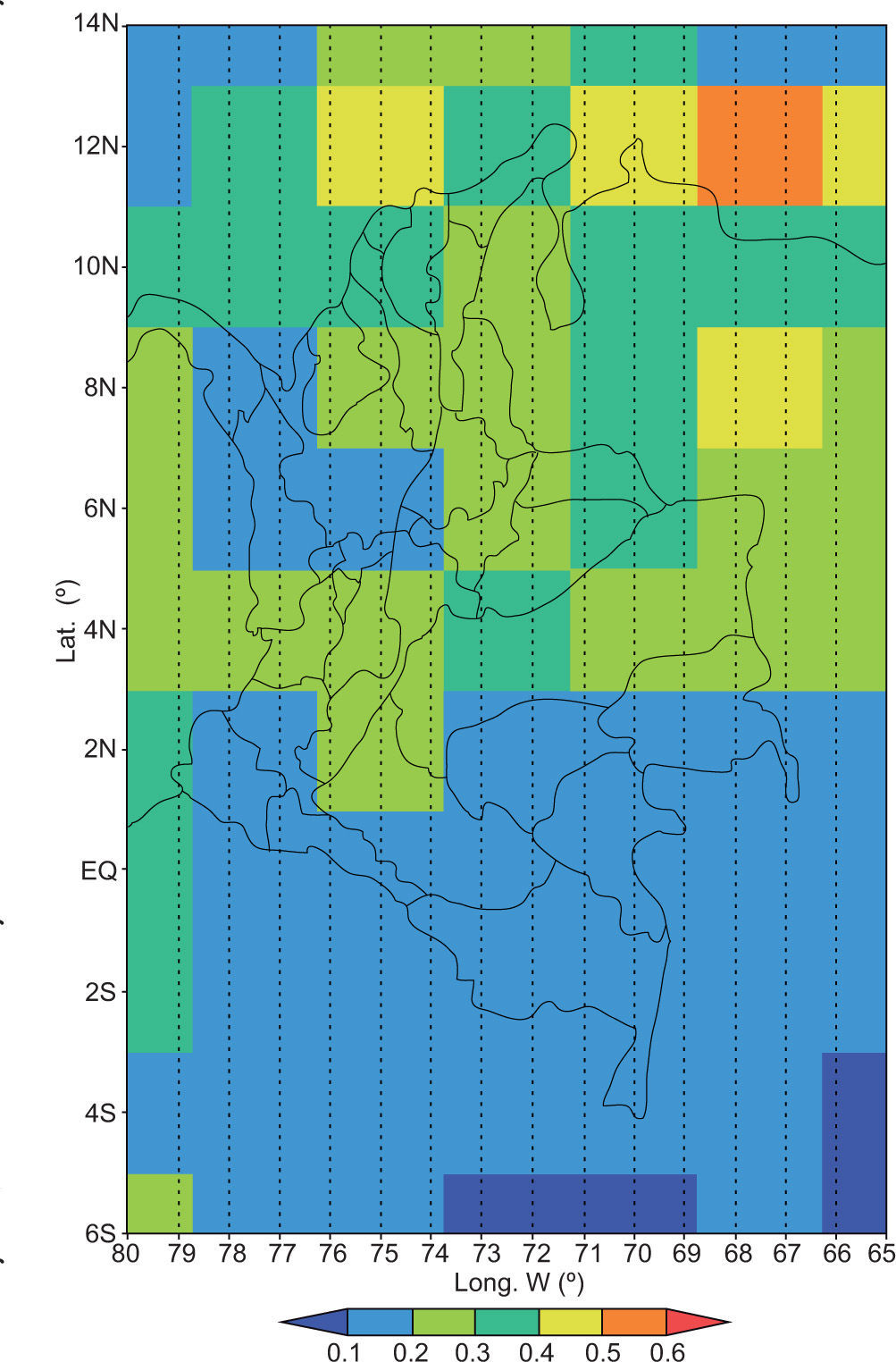
Figure 8 shows the CF obtained through GEOS-Chem simulation for February 2007 using Eq. (4). The values shown represent the monthly average for the period between 12:00 and 14:00 LT. We show CF only for one month because there is very little variability from month to month. Throughout most of Colombia, the CF values range from less than 0.2 to 0.4. This finding indicates an overestimation in the NO2 reading by the molybdenum catalytic converter of between 60 and 80%, which implies that a large reservoir of NO2 is present in NOy species, such as PAN, HNO3, and alkyl nitrates. Because Colombia is located in the equatorial zone, a high level of solar radiation is present during most of the year, and this result is comparable to that reported by Lamsal et al. (2008) for North America in the summer season. Lamsal et al. (2008) found lower CF values in summer, with values of approximately 0.2 being predominant in regions with low anthropogenic activity. This result is due primarily to the short lifetime of NO2 given the influence of solar radiation during the day, which favors the conversion of NO2 to NO following the exhaustion reaction:
 for February 2007 for the interference in the commercial meters used for measuring surface NO2 in situ.")
During the day, NO is present in higher levels than NO2, and during the night, the converse is true.
Another important factor that affects the value of CF is anthropogenic activity, which is related to the population density and the industrial characteristics of a region. In general, the higher the levels of anthropogenic activity, the higher the concentrations of NOx species. In remote regions, the levels of anthropogenic activity are lower and NOy compounds prevail. From the center of Colombia to the north (i.e., in the region with the highest anthropogenic activity), the CF values are slightly higher compared with the CF values in the southern and southeastern parts of the country (which include departments with smaller populations, such as Amazonas, Guainía, Caquetá, Putumayo, and Guaviare). The highest values for all months (between 0.4 and 0.6) occur close to the Venezuelan coast, probably due to anthropogenic causes.
4.7OMI-derived NO2 concentrations versus in situ and biomass burning data4.7.1Comparison of OMI-derived NO2 concentrations and in situ concentrationsCorrelation coefficients were calculated for the comparison of the monthly mean surface NO2 concentrations measured in situ with those inferred from OMI data. For each in situ data point, it was necessary to apply the correction factor in the GEOS-Chem grid that was closest to the associated measuring station. Data were only available from seven ground stations in two cities: Bogotá (six stations) and Bucaramanga (one station). Several main cities such as Medellín (Antioquia), Pereira (Risaralda), Manizales (Caldas), and Cali (Valle del Cauca) have air quality monitoring networks; however, we could only have access to the data for Bogotá and Bucaramanga. On the other hand, cities that have air quality monitoring networks are located west of the Cordillera Oriental, so that in much of the country, no surface stations exist from which air quality data can be obtained to study the sources and transport mechanisms of pollutants in Colombia.
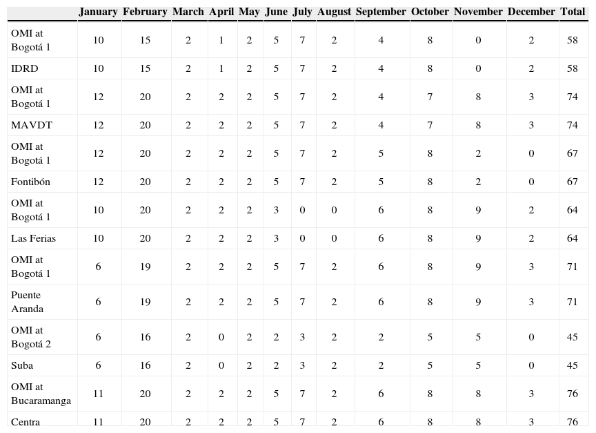
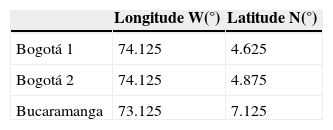
The stations located and used in Bogotá are IDRD, MAVDT, Fontibón, Las Ferias, Puente Aranda, and Suba. The station located and used in Bucaramanga is Centro. The number of data points used simultaneously for inferred monthly NO2 concentrations and measuring stations in Bogotá and Bucaramanga is presented in Table II. As can be observed in this table, certain averages were calculated using only one simultaneous data point, and in the best case, some averages were calculated using 20 simultaneous data points. Since Bogotá has an area of 1600 km2, two OMI grid cells at the resolution 0.5 × 0.5º were used to compare with the station data. The location of the midpoint of each grid cell is shown in Table III.
Number of daily data points available simultaneously for calculation of the monthly average N02 concentrations from the OMI and from the surface stations in Bogotá and Bucaramanga.
| January | February | March | April | May | June | July | August | September | October | November | December | Total | |
|---|---|---|---|---|---|---|---|---|---|---|---|---|---|
| OMI at Bogotá 1 | 10 | 15 | 2 | 1 | 2 | 5 | 7 | 2 | 4 | 8 | 0 | 2 | 58 |
| IDRD | 10 | 15 | 2 | 1 | 2 | 5 | 7 | 2 | 4 | 8 | 0 | 2 | 58 |
| OMI at Bogotá 1 | 12 | 20 | 2 | 2 | 2 | 5 | 7 | 2 | 4 | 7 | 8 | 3 | 74 |
| MAVDT | 12 | 20 | 2 | 2 | 2 | 5 | 7 | 2 | 4 | 7 | 8 | 3 | 74 |
| OMI at Bogotá 1 | 12 | 20 | 2 | 2 | 2 | 5 | 7 | 2 | 5 | 8 | 2 | 0 | 67 |
| Fontibón | 12 | 20 | 2 | 2 | 2 | 5 | 7 | 2 | 5 | 8 | 2 | 0 | 67 |
| OMI at Bogotá 1 | 10 | 20 | 2 | 2 | 2 | 3 | 0 | 0 | 6 | 8 | 9 | 2 | 64 |
| Las Ferias | 10 | 20 | 2 | 2 | 2 | 3 | 0 | 0 | 6 | 8 | 9 | 2 | 64 |
| OMI at Bogotá 1 | 6 | 19 | 2 | 2 | 2 | 5 | 7 | 2 | 6 | 8 | 9 | 3 | 71 |
| Puente Aranda | 6 | 19 | 2 | 2 | 2 | 5 | 7 | 2 | 6 | 8 | 9 | 3 | 71 |
| OMI at Bogotá 2 | 6 | 16 | 2 | 0 | 2 | 2 | 3 | 2 | 2 | 5 | 5 | 0 | 45 |
| Suba | 6 | 16 | 2 | 0 | 2 | 2 | 3 | 2 | 2 | 5 | 5 | 0 | 45 |
| OMI at Bucaramanga | 11 | 20 | 2 | 2 | 2 | 5 | 7 | 2 | 6 | 8 | 8 | 3 | 76 |
| Centra | 11 | 20 | 2 | 2 | 2 | 5 | 7 | 2 | 6 | 8 | 8 | 3 | 76 |
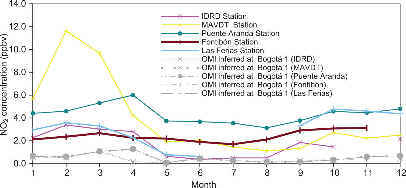
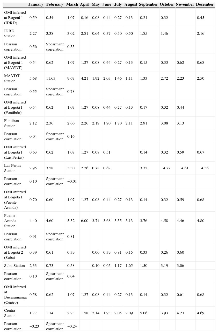
Monthly averages and correlations for stations in Bucaramanga and Bogotá are presented in Table IV. The in situ data that are most highly correlated with the OMI inferred data are those from the Puente Aranda, IDRD and MAVDT stations. Data from these three stations yield Pearson coeffcients of 0.91, 0.56 and 0.55 and Spearman coefficients of 0.81, 0.55 and 0.78, respectively. The stations with the highest annual mean are Puente Aranda, MAVDT and Las Ferias, in that order. It is noted that the Puente Aranda station is located in the second-biggest industrial zone in Colombia, which could mean that concentration of polluting agents, in particular NO2, could be homogeneous in the surrounding area represented by the corresponding OMI grid cell (Bogotá 1), so that Puente Aranda could have the best local background measurements relative to the other stations.
Monthly average surface concentrations of N02 (in ppbv) inferred from OMI data using Eq. (2) and corrected measurements at the stations in Bogotá and Bucaramanga.
| January | February | March | April | May | June | July | August | September | October | November | December | |
|---|---|---|---|---|---|---|---|---|---|---|---|---|
| OMI inferred at Bogotá 1 (IDRD) | 0.59 | 0.54 | 1.07 | 0.16 | 0.08 | 0.44 | 0.27 | 0.13 | 0.21 | 0.32 | 0.45 | |
| IDRD Station | 2.27 | 3.38 | 3.02 | 2.81 | 0.64 | 0.37 | 0.50 | 0.50 | 1.85 | 1.46 | 2.16 | |
| Pearson correlation | 0.56 | Spearmann correlation | 0.55 | |||||||||
| OMI inferred at Bogotá 1 (MAVDT) | 0.54 | 0.62 | 1.07 | 1.27 | 0.08 | 0.44 | 0.27 | 0.13 | 0.15 | 0.33 | 0.62 | 0.68 |
| MAVDT Station | 5.68 | 11.63 | 9.67 | 4.21 | 1.92 | 2.03 | 1.46 | 1.11 | 1.33 | 2.72 | 2.23 | 2.50 |
| Pearson correlation | 0.55 | Spearmann correlation | 0.78 | |||||||||
| OMI inferred at Bogotá I (Fontibón) | 0.54 | 0.62 | 1.07 | 1.27 | 0.08 | 0.44 | 0.27 | 0.13 | 0.17 | 0.32 | 0.44 | |
| Fontibon Station | 2.12 | 2.36 | 2.66 | 2.26 | 2.19 | 1.90 | 1.70 | 2.11 | 2.91 | 3.08 | 3.13 | |
| Pearson correlation | 0.04 | Spearmann correlation | 0.16 | |||||||||
| OMI inferred at Bogotá I (Las Ferias) | 0.63 | 0.62 | 1.07 | 1.27 | 0.08 | 0.51 | 0.14 | 0.32 | 0.59 | 0.67 | ||
| Las Ferias Station | 2.95 | 3.58 | 3.30 | 2.26 | 0.78 | 0.62 | 3.32 | 4.77 | 4.61 | 4.36 | ||
| Pearson correlation | 0.10 | Spearmann correlation | −0.01 | |||||||||
| OMI inferred at Bogotá I (Puente Aranda) | 0.70 | 0.60 | 1.07 | 1.27 | 0.08 | 0.44 | 0.27 | 0.13 | 0.14 | 0.32 | 0.59 | 0.68 |
| Puente Aranda Station | 4.40 | 4.60 | 5.32 | 6.00 | 3.74 | 3.68 | 3.55 | 3.13 | 3.76 | 4.58 | 4.46 | 4.80 |
| Pearson correlation | 0.91 | Spearmann correlation | 0.81 | |||||||||
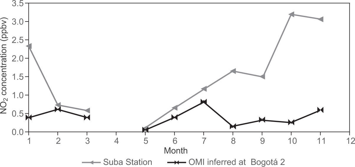
| OMI inferred at Bogotá 2 (Suba) | 0.39 | 0.61 | 0.39 | 0.06 | 0.39 | 0.81 | 0.15 | 0.33 | 0.26 | 0.60 | ||
| Suba Station | 2.33 | 0.73 | 0.58 | 0.10 | 0.65 | 1.17 | 1.65 | 1.50 | 3.19 | 3.06 | ||
| Pearson correlation | 0.10 | Spearmann correlation | 0.04 | |||||||||
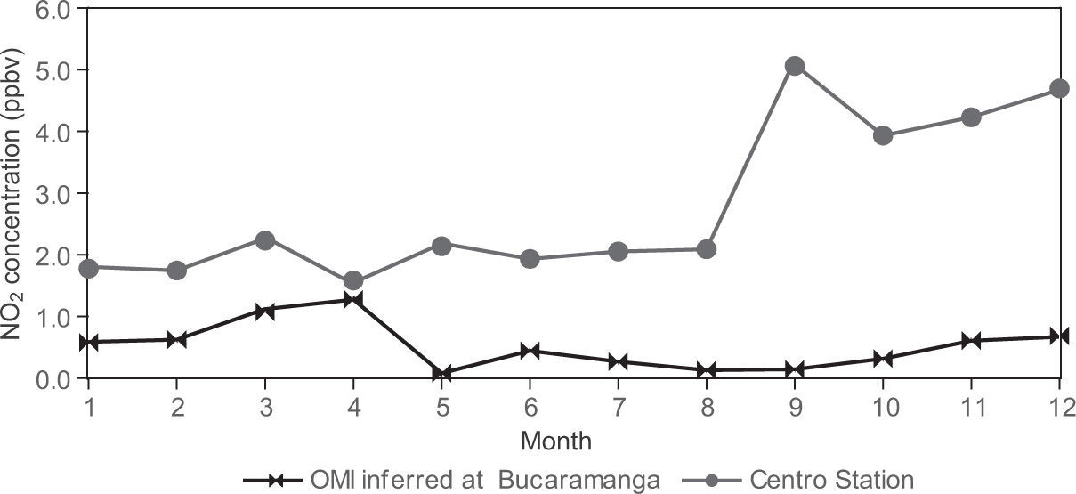
| OMI inferred at Bucaramanga (Centro) | 0.58 | 0.62 | 1.07 | 1.27 | 0.08 | 0.44 | 0.27 | 0.13 | 0.14 | 0.32 | 0.61 | 0.68 |
| Centra Station | 1.77 | 1.74 | 2.23 | 1.58 | 2.14 | 1.93 | 2.05 | 2.09 | 5.06 | 3.93 | 4.23 | 4.69 |
| Pearson correlation | −0.23 | Spearmann correlation | −0.24 |
Figures 9-11 show the monthly means of NO2 concentrations from the stations in Bogotá and Bucaramanga and the corresponding inferred OMI values. The NO2 concentrations inferred from OMI data for Colombia are similar to those found by Lamsal et al. (2008) in the U.S. for the summer season. These authors reported NO2 concentrations of 0.1 ppbv in rural regions and between 2 and 3 ppbv in urban areas. Since the measurements at the stations are at surface level, they do not reflect the influence of either the mixed layer or the horizontal atmospheric movements, both of which serve to mix atmospheric pollutants. Thus, inferred OMI NO2 concentration tends to be lower than point measurements reported at the corresponding stations. Therefore, the values for the stations reported in Figures 9-11 could have overestimations even though they correspond to corrected data according to the CF obtained from GEOS-Chem (section 4.6). Such CFs are influenced by the interferences caused mainly by NOy species such as PAN, alkyl nitrates and HNO3 (see Eq. 4). Thus, it can be expected that, despite the correction, surface NO2 concentrations from the stations are still overestimated. It is therefore desirable to determine the conversion rates of interfering NOy species. The conversion of HNO3 is not easy to resolve and depends on the measuring equipment, as noted by Lamsal et al. (2008), who reported a value of 35%. In the cases of PAN and alkyl nitrates, conversion to more stable compounds is expected (Steinbacher et al., 2007). On the other hand, a main reason for the underestimation of satellite-inferred concentrations is the limited sensitivity of the remote sensing instrument close to the surface.
 at Bogotá 1 inferred from OMI data using Eq. (2) and from corrected measurements at the IDRD, MAVDT and Puente Aranda, Fontibón and Las Ferias stations, which are located in Bogotá. All the curves correspond to values in Table IV.")
 at Bogotá 2 inferred from OMI data using Eq. (2) and from corrected measurements at Suba station, which is located in Bogotá.")
Monthly average surface concentrations of NO2 (in ppbv) at Bogotá 2 inferred from OMI data using Eq. (2) and from corrected measurements at Suba station, which is located in Bogotá.
 at Bucaramanga inferred from OMI data using Eq. (2) and from corrected measurements at Centro station, which is located in Bucaramanga.")
Monthly average surface concentrations of NO2 (in ppbv) at Bucaramanga inferred from OMI data using Eq. (2) and from corrected measurements at Centro station, which is located in Bucaramanga.
It should also be noted that our data validation process was limited because a high layer of cloud cover is usually present over the mountainous regions. This cloud cover impedes the measurement of NO2 columns in the visible spectrum (section 2.1) and as can be observed on the map in Figure 12, the lack of data for the Andean region (departments of Nariño, Cauca, Valle del Cauca, Huila, Tolima, Risaralda, Quindío, Cundinamarca, Antioquia, Boyacá, Santander and Norte de Santander) is considerable. The scarcity of data for the mountainous regions is not unique to 2007. Similar patterns are evident for the years 2008 and 2009 (not shown). Unfortunately, the surface measurement stations available to provide data useful for validation are located in a mountainous and cloudy area. Six of the seven stations are located in Bogotá, which is located in the Andean region and has an elevation of 2600 m. The seventh station is located in Bucaramanga, which is also located in the Andean region and has an elevation of 959 m. The extension of the network of surface measurement stations to both remote and new urban areas would enable more comprehensive measurement of background concentrations of NO2 and would facilitate a more complete validation throughout Colombia.
4.7.2Estimated NO2 surface concentration vs. MACC Fire Radiative Power
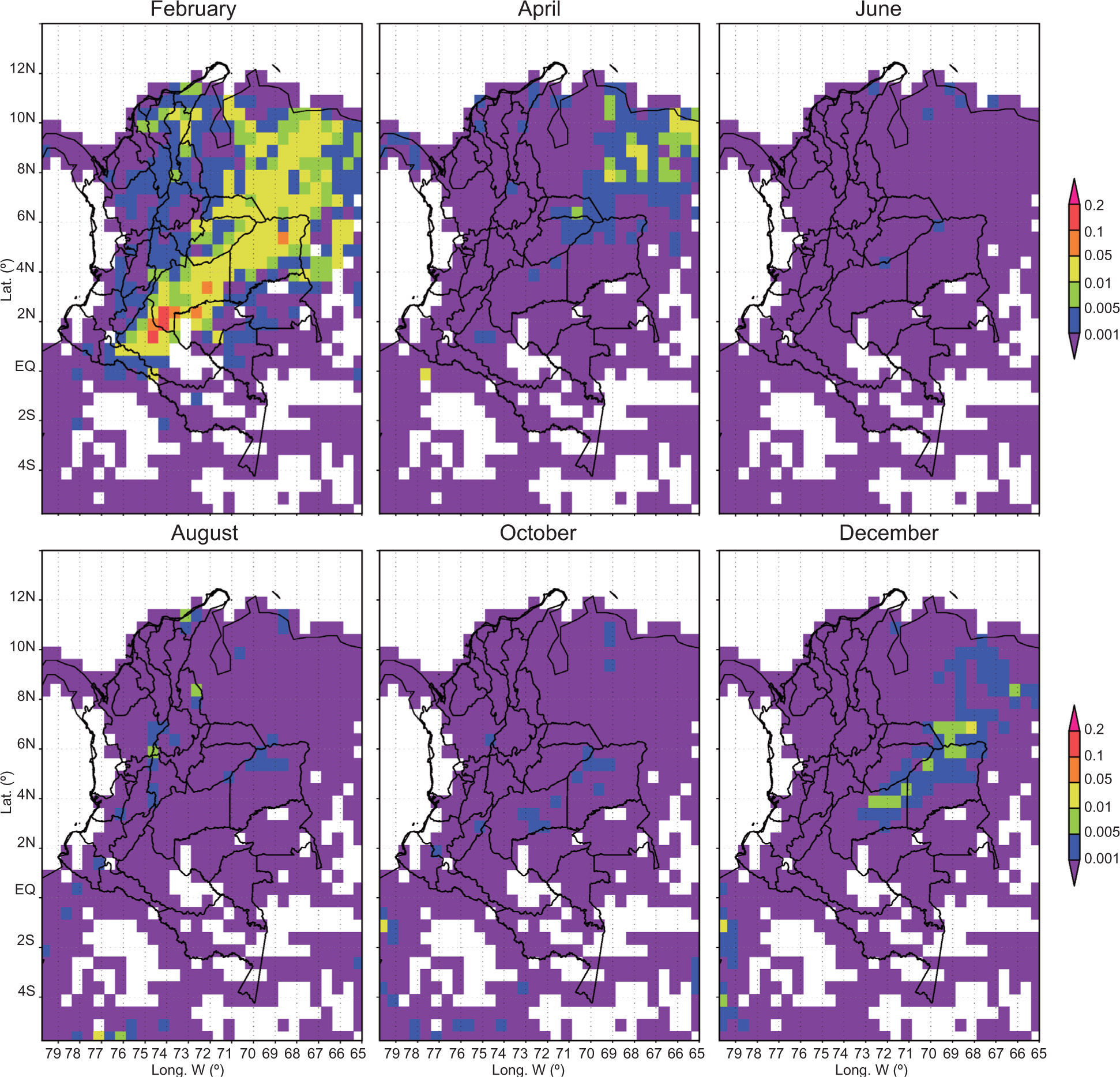
Fire radiative power (FRP) determines the burning rate of biomass (living and dead vegetation). The Global Fire Assimilation System (GFASv1.0) calculates biomass-burning emissions by assimilating FRP observations from the MODIS instrument onboard the Terra and Aqua satellites (Kaiser et al., 2012). We used the FRP data from the Daily Wildfire Emissions product provided by the Monitoring Atmospheric Composition & Climate (MACC) project (available at http://macc.iek.fz-juelich.de/data/compressed/orig/MACC_Daily_Wildfre_Emissions/). FRP daily data has a horizontal spatial resolution of 0.5 × 0.5º (latitude × longitude), and has been produced since 2003 to the present.
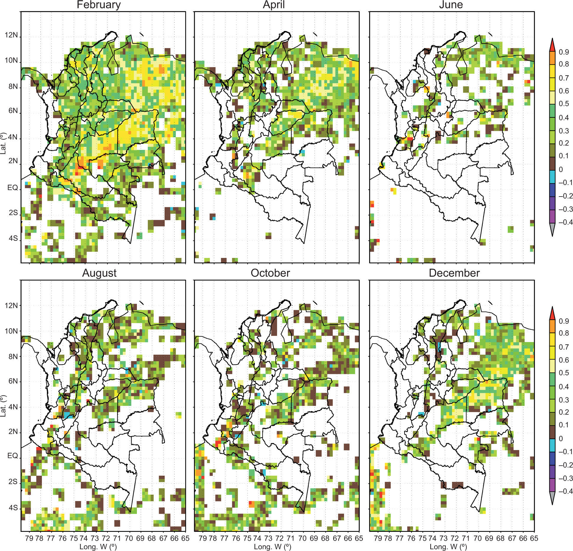
Figure 13 shows monthly means of FRP for 2007. It can be noted that a high amount of biomass was burned in Colombia in February (and also in January and March [not shown]), while biomass burning was scarce in the months after. Figure 14 shows maps of correlation between FRP and OMI-de-rived NO2 surface concentration estimated in section 4.5. The biggest number of grid points with high correlation values (> 0.5) is observed for February (and also in January and March [not shown]), especially in Vichada, Meta, Guaviare, Caquetá, and the western part of Venezuela, regions where the prevailing biome is humid tropical forest. This implies that the high NO2 concentrations in Figure 7 in these regions are mostly attributable to biomass burning. The correlations are low in the months after. In Cesar, Magdalena, Bolívar, and La Guajira, where the prevailing biome is tropical dry forest, there are intermediate values of FRP (Fig. 13). The correlation values between FRP and the estimated NO2 surface concentration (Fig. 14) in these regions suggest that the NO2 concentrations are partially due to biomass burning and partially due to industrial NO2 generating processes.

 that the requirement of having a minimum of 12 daily non-missing simultaneous values is not met, or (2) that FRP daily values are equal to zero for the whole year. The second situation is to be found, e.g., over the sea. Only the maps for even months are shown.")
Correlation maps between inferred NO2 surface concentration and FRP interpolated to the 0.5 × 0.5º resolution. For these correlation maps a minimum number of non-missing daily values for each variable in each grid point was taken into account; this number is equal to 12. Correlations equal to or higher than 0.5 are statistically significant at the 90% level. Blank grid boxes represent either: (1) that the requirement of having a minimum of 12 daily non-missing simultaneous values is not met, or (2) that FRP daily values are equal to zero for the whole year. The second situation is to be found, e.g., over the sea. Only the maps for even months are shown.
1. There is an overestimation of OMI columns in remote regions. We propose that on remote regions, where the density of OMI NO2 columns is expected to be very low, the amount of 0.4 × 10¹⁵ molecules/cm2 should be subtracted.
2. The inferred NO2 concentration values are relatively low (between 0.01 and 0.5 ppbv) throughout most of the country. However, relatively high concentrations (between 3 and 4 ppbv) occur in the departments of Caquetá and Meta in February. A main reason for the underestimation of satellite-inferred concentrations is the limited sensitivity of the remote sensing instrument close to the surface.
3. The comparison of NO2 concentrations inferred from OMI data and those based on ground station measurements from the stations Puente Aranda, IDRD and MAVDT in Bogotá yields Pearson correlation coefficients of 0.91, 0.56 and 0.55 and Spearman coefficients of 0.81, 0.55 and 0.78, respectively.
4. The comparison of the NO2 concentrations inferred from OMI data and FRP yields high correlation coefficients in areas where the concentrations are high. These areas are tropical rainforests. This indicates that these high NO2 concentrations are due to biomass burning, which includes the human-initiated burning of vegetation for land clearing and land use change as well as natural, lightning-induced fires. In areas with correlations between 0.4 and 0.7 (located in western Venezuela and central and northern Colombia during February), NO2 concentrations can be partially associated with biomass burning and partially with other processes such as transport of NO2 or its precursors from other regions, burning of fossil fuels by the oil industry, and diverse industrial processes.
This work is supported by the Proyecto Piloto Nacional de Adaptación al Cambio Climático (INAP, National Pilot Project on Adaptation to Climate Change) and the Dirección de Investigaciones Sede Bogotá (DIB, Directorate of Research of Bogotá) of the Universidad Nacional de Colombia through the Convocatoria Nacional de Investigación y Creación Artística 2010-2012 (National Call for Research and Artistic Creation 2010-2012).