


As global economic integration accelerates and international trade grows increasingly complex, trade demand shocks have emerged as a critical factor shaping the resilience of global industrial chains. This study develops a risk identification–resilience evolution–cost recovery framework to analyze the dynamic impact of demand-side trade shocks on industrial chain resilience. We model the effects of trade demand shocks on the inoperability of industrial chains using bi-regional input–output tables for China and the United States (US) to assess the resilience and robustness of sectors. This is achieved by constructing static and dynamic decision models and quantifying economic loss under various investment scenarios. The study analyzes three investment portfolios to examine how investment strategies impact the resilience of Chinese and US industries. The results provide targeted guidance for cross-regional industrial chain risk management, revealing that Chinese and US investments complement one another. China should prioritize manufacturing investment to support short-term recovery and long-term resilience, and the US should focus on the service sector, which has a crucial influence on economic fluctuations and overall stability. These findings offer valuable insights for policymakers seeking to mitigate the impact of external demand shocks while strengthening the international competitiveness and resilience of industrial chains.
The contemporary global economy is facing severe challenges, including slowing economic growth, the rise of protectionism and unilateralism, commodity price fluctuations, increased instability and uncertainty, and a significant increase in external import risk (Li & Fang. 2024; Hao et al. 2024). Therefore, effective risk management is crucial for sustaining global value chains (Heckmann et al. 2015). Since the outbreak of the Sino–US trade war in 2018, a series of tariffs and nontariff measures have reshaped global supply and industrial chains. In response, the Chinese government has implemented countermeasures, including tariff policies, industrial support, and international cooperation. For example, China has tariffs on imports from the United States (US), ranging from US$34 billion to US$200 billion, with tariffs involving agriculture, machinery, chemicals, steel, aluminum, and other industries generally spanning from 5 % to 25 % (Bown et al., 2021). Rather than detailing the entire policy chronology, this study focuses on how such trade tensions function as persistent exogenous shocks, posing significant risks to industrial chain stability. These external demand shocks pose significant challenges to the economic stability of China and the US and the entire global economy. In this context, examining the industrial chain resilience in China and the US under trade demand shocks is increasingly crucial. Therefore, risk management and industrial chain resilience have become critical research areas. For example, Rostamzadeh et al. (2018) proposed multicriteria decision-making methods to assess and manage sustainable supply chain management risks. However, many studies have remained limited by fragmented approaches that lack integration across risk identification, dynamic resilience evolution, and cost recovery trajectories, particularly through the lens of organizational practices and decision-making when confronting uncertainty (Matyas & Pelling, 2015). Additionally, standardized metrics and sector-specific recovery mechanisms under sustained demand shocks have been insufficiently explored.
Recent studies highlight the role of resilience in mitigating disruptions and fostering sustainable economic development (Abdel-Basset & Mohamed, 2020; Katsaliaki et al., 2022). Hosseini et al. (2020) and Pettit et al. (2010) expanded resilience measurement research and applied it to small and medium-sized enterprises’ management decisions. However, the absence of standardized metrics has led to inconsistent definitions of industry chain resilience, undermining the comparability and generalizability of findings. Most studies rely on static analyses (Hu & Zhang, 2023), failing to address the dynamic evolution of resilience under extreme external shocks or the mechanisms of recovery. Furthermore, traditional risk management approaches treat resilience and risk as separate constructs, overlooking their dynamic interplay (Liu et al. 2024). Moreover, previous research has not examined the interaction between risk identification and the evolution of resilience. Addressing this gap is essential for advancing both the theoretical and practical understanding of industrial chain resilience.
This study addresses three research questions. (1) How do trade demand shocks affect static and dynamic resilience indicators? (2) How does recovery vary between sectors in different countries? (3) How do different investment portfolios and strategies influence cost-effective recovery?
To answer these critical questions, we propose an integrated risk identification–resilience evolution–cost recovery framework for industrial chain risk management that systematically connects static sensitivity, dynamic recovery, and managerial decision-making. The proposed framework provides a more comprehensive basis for understanding and managing industrial chain resilience under complex trade demand shocks. The main contributions of this paper are threefold. (1) The study quantitatively assesses the resilience trajectory and economic loss of Chinese and the US industrial chains under trade demand shocks. (2) We develop and validate a static–dynamic–decision space risk management framework that integrates risk identification, resilience evolution, and cost recovery. (3) The results provide clear policy and managerial recommendations that align with sector-specific strengths and promote robust, adaptive recovery strategies for managing continued global trade risks. By explicitly addressing research gaps, this study contributes to advancing theoretical understanding and practical applications for industrial chain resilience, supporting policymakers and industry leaders navigating an increasingly uncertain global economic environment.
Literature review and research approachAmid growing uncertainty regarding the global economy and US–China trade tensions, industrial chain resilience has become a critical research theme. In this section, we review recent advances in industrial chain resilience research, focusing on three key areas of theoretical foundation, measurement methods, the impact of exogenous shocks in relation to this study’s approach.
Theoretical foundationThe concept of industrial chain resilience originates from the integration of “industry chain” and “resilience.” While it draws on the analytical approaches to economic resilience, it also incorporates distinctive implications for industrial chain dynamics. Its theoretical foundation is firmly rooted in broader theories of industrial organization and economic linkages. Hirschman’s (1958) linkage effects theory highlights the upstream and downstream interdependencies among sectors, while Gereffi et al. (2005) emphasize the governance of global value chains, underscoring the role of interfirm linkages and institutional contexts in shaping competitiveness and resilience. Collectively, these perspectives suggest that an industrial chain is not merely a collection of independent supply chains but rather a complex, interdependent system through which shocks can propagate across multiple transmission channels.
Subsequent studies extended this framework to incorporate adaptive learning and proactive capacity (Bruneau et al., 2003; Rice & Caniato, 2003; Ponomarov & Holcomb, 2009). Martin’s (2012) four-dimensional framework of regional resilience—resistance, recovery, reorganization, and renewal—provides an important analytical framework for understanding the dynamic processes of industrial chain resilience, illustrating how economic systems absorb shocks, adjust to disruptions, and evolve. Since then, research on industrial chain resilience has shifted from static analysis to in-depth exploration of evolutionary mechanisms and path identification, significantly advancing the field (Dormady et al., 2019; Liu et al., 2024). Contemporary research has increasingly emphasized the importance of embedding resilience within dynamic systems that facilitate continuous adaptation and improvement (Domingos et al., 2024).
Industrial chain resilience is intrinsically connected to input–output theory. The input–output model highlights sectoral interdependencies and the transmission of shocks across industries, making it a powerful tool for analyzing the structural characteristics of industrial systems. Acemoglu et al. (2012) demonstrated that microlevel shocks can be amplified into macroeconomic risks through the topology of production networks, providing a rigorous theoretical foundation for resilience assessment based on input–output structures. Building on this, studies of complex adaptive systems (Barabási, 2009) demonstrate that network topology, feedback loops, and adaptive interactions determine whether local disruptions escalate into systemic crises. This perspective situates industrial chain resilience within the broader literature on complex systems and systemic risk.
Moreover, the resilience of industrial chains is increasingly recognized as a fundamental aspect of risk management. From a supply chain risk management perspective (Christopher & Peck, 2004), resilience entails the capability to identify, assess, and mitigate risks while ensuring continuity of operations. This links resilience not only to postdisruption recovery but also to proactive strategies of vulnerability mitigation and the enhancement of adaptive capacity. Integrating resilience theory with risk management frameworks provides a more comprehensive understanding of how industrial systems respond to exogenous shocks (Tang, 2006).
Measurement methodsIn the existing literature, industry chain resilience is primarily assessed using three methodological approaches: the core variable method, the comprehensive evaluation method, and the input–output method. (1) core variable method. The core variable method is a commonly employed approach in the study of economic resilience, which characterizes resilience dynamics by identifying a single representative variable and constructing a relative variability index. For example, Jiang et al. (2023) employ stock returns to capture the level of firm resilience. Building on this idea, several scholars in industry chain research have employed the core variable method to evaluate industry chain resilience. Di Tommaso et al. (2023) conceptualized “industry resilience” and employed employment data from the US. Department of Labor Bureau of Labor Statistics to measure resilience levels across industries. By constructing relative change indicators of employment, they assessed industry resilience in terms of both resistance and recovery capacity. (2) the comprehensive evaluation method. The comprehensive evaluation method refers to the overall assessment of multiple indicators in complex systems. It relies on multicriteria decision-making (MCDM) tools to address and evaluate complex decision problems. MCDM approaches have been widely applied in resilience research (Briguglio et al., 2009; Bolson et al., 2022). The comprehensive evaluation method is primarily suited for describing resilience at a macro, static level. However, it does not capture the dynamic characteristics of individual nodes at the micro level, such as their resistance and response capacities. (3) input–output model. The input–output model enables the tracing of economic flows using empirical data, facilitating the analysis of interdependencies among sectors and regions. This capability has drawn substantial attention from scholars in supply chain, value chain, and production network research, and has increasingly been extended to the study of industrial chains. These findings provide a theoretical basis for assessing resilience through input–output structures. A key advantage of employing the input–output model to study industrial chain resilience is its ability to capture the interindustry associations and accurately flow value among different production links, effectively representing the “chain attributes” of the industrial system.
Impact of exogenous shocksIn response to rising global uncertainty, scholars have increasingly investigated the impact of exogenous shocks on industrial chain resilience. Existing studies have mainly concentrated on identifying the types of shocks and their corresponding transmission mechanisms. Classification frameworks developed by Hernes et al. (2022) established a theoretical approach for identifying shock types and predictability. To investigate transmission mechanisms, Ikeda and Iyetomi (2018) proposed a model to examine the structural effects of trade policy changes on global trade networks, and Garvey et al. (2015) used a Bayesian network approach to simulate the impact of external shocks. Additionally, research has begun to link risk with resilience by focusing on risk identification, assessment, and mitigation strategies (Brandon-Jones et al. 2014; Ali et al. 2024). Logan et al. (2022) proposed an analytical framework for enhancing resilience in integrated systems. Research on external shocks continues to evolve, yielding increasingly significant theoretical and practical implications.
Current research on industrial chain resilience and risk management remains limited, often offering only superficial definitions that overlook the nature, structure, and interconnections of industrial chains. This gap hinders a comprehensive understanding of resilience across industries and regions when faced with external shocks. Resilience measurement lacks standardization, with varied concepts and indicators complicating the quantification of dynamic risk interactions. Most studies are static, missing the evolution of resilience and mechanisms for resistance and recovery from demand shocks. Additionally, resilience and risk are often studied separately, ignoring their interdependencies and cost implications. In response, we propose a novel risk identification–resilience evolution–cost recovery framework that explicitly links demand shocks to resilience trajectories and the associated recovery costs through input–output modeling. This approach advances the research by addressing the dynamic interaction between risk and resilience and reveals actionable insights for policymakers and managers facing complex global shocks.
Research designTheoretical background and research frameworkThis study combines dynamic and static input–output modeling to analyze industrial chain resilience under exogenous trade shocks using an inoperability input–output model (IIM) and a dynamic input–output model (DIIM). To strengthen its theoretical anchoring, the framework draws on organizational contingency theory, which suggests that managerial strategies should adapt to external uncertainty (Donaldson, 2001). Our decision space design offers a strategic managerial tool for optimizing resource allocation and recovery actions under different shock scenarios, which is consistent with previous research on decision-making amid uncertainty (March & Shapira, 1987).
The core framework follows a static–dynamic–decision space progression. First, our static analysis quantitatively assesses the industrial chain’s initial resilience to external shocks, identifying system sensitivity to investment and providing a foundation for subsequent risk management decision-making. Second, our dynamic analysis examines the postshock recovery and resilience process, quantifying key indicators such as recovery speed and cycle time. Finally, our proposed decision space for resilience risk management integrates static and dynamic insights, analyzing the impact of alternative recovery strategies on short-term stability and long-term performance. The results offer quantitative support for optimizing resource allocation and enhancing industrial chains’ shock resistance and recovery capacity.
Overall, our proposed integrated framework bridges quantitative modeling with organizational behavior theory, providing theoretical and practical insights for risk management under complex trade disruptions.
Inoperability input–output modelThe IIM extends the traditional input–output model to analyze how irregularities propagate across interrelated industrial sectors. The basic equation is expressed as follows:
where q indicates the degree of inoperability, which measures the extent to which the infrastructure or industry sector does not function as planned. For n interrelated sectors, X^ and C^ denote the planned aggregate output and final demand at equilibrium, X˜ and C˜ represent the equilibrium of aggregate output and final demand following the shock. Therefore, the respective expressions for inoperability (q) and demand shock (c*) are q=[diag(x^)]−1(x^−x˜) and c*=[diag(x^)]−1(c^−c˜).
We define [diag(x^)]−1A[diag(x^)] as matrix A*, which represents the degree of economic–technological interdependence between industrial sectors. The key assumption of our proposed model is that the structure of economic interdependence, denoted by the matrix A*, remains unchanged when aggregate demand satisfaction and the resulting output change.
Dynamic inoperability input–output modelWe use the general DIIM proposed by Miller and Blair (2009) as follows:
where B is a matrix of investment coefficients, which measures the public sector’s willingness to invest capital in different sectors. When the DIIM reaches equilibrium, i.e. x˙(t)=0, a modified traditional dynamic input–output model sets B=−I to use the model as an adjustment mechanism that determines supply–demand imbalance in the economy’s output at time t (Haimes et al. 2005).
We introduce the recovery coefficient k to adjust the supply–demand imbalance and reach a state at which aggregate output and aggregate demand are in equilibrium at time t. Here, K=diag(k1,…,kn) is the diagonal matrix of industrial sectors’ recovery coefficients, and the nonzero diagonal element ki of the ith sector is defined as the industrial recovery coefficient that indicates the sector’s ability to recover from a disturbance. The matrix of industrial recovery coefficients determines industrial sectors’ exponential dynamic evolution, where a larger ki value indicates faster economic system reaction to the supply–demand imbalance.
Then, the general formula for our proposed DIIM is as follows:

The DIIM incorporates industrial sectors’ interdependence, the stochastic nature of the dynamic process, and the theoretical foundations of the IIM model. Equation (3) is the standard form of a first-order differential equation, and its solution can be obtained as follows when the initial value of q(0) is obtained:

Equation (4) is solved assuming that the c*(t) perturbation of final demand is fixed as follows:

If time is discrete, the demand-driven DIIM can also be represented in the form of the following difference equation:

We next analyze the DIIM dynamics of the recovery process after a disruption of production in the industrial sector caused by an external shock. Following an external shock, economic output (x(t)) decreases to a smaller x˜(t). When final demand is held constant, the sector’s aggregate demand (Ax˜(t)+C(t)) will exceed the sector’s output x˜(t), after which the affected sector gradually recovers its production capacity, and the demand–supply imbalance (Ax˜(t)+C(t)−x˜(t)) progressively narrows until the sector recovers its ability to supply sufficient output to meet aggregate demand.
When an external shock occurs, aggregate output in the economic sector begins to decrease, resulting in the sector’s inability to function properly (q(0) > 0), assuming that aggregate demand in each industrial sector remains unchanged following the shock (c*=0). Equation (5) can be simplified as follows:

The above equation describes the economic system’s dynamic recovery process when output changes while final demand remains constant. As t→∞, q(∞)=0, indicating that the economic sector can gradually recover from its functionally constrained initial state to full normal operation with sufficient recovery time. Therefore, a longer recovery time indicates a higher likelihood that the economic system will stabilize after an external shock, achieving resilient recovery of the entire system.
In analyzing the rate of recovery of the sector, we assume that industrial sector i recovers from the initial perturbation qi(0)>0 to a new state qi(Ti) after time Ti and brings supply and demand to a new equilibrium state. At this point, the following relationship can be obtained from equation (7):

As shown in equation (8), the actual recovery rate of industrial sector i includes two components. One is the sector’s own recovery rate, and the other is the recovery rate influenced by other sectors. This indicates that the sector’s recovery depends on its own capacity as well as that of related sectors.
Recovery rate K has a range of (0, 1), and values within this range ensure that K(I−A*) has positive eigenvalues, which is a necessary condition to ensure that the solution of equation (4) does not diverge and can converge to a stable state when performing dynamic modeling to conduct an effective assessment of the industrial chain’s resilience.
Building on this, the next section introduces the set of dynamic resilience indicators used to assess the cost of industrial chain adjustment to meet actual demand in response to contingencies and corresponding risk management strategies.
Industrial Chain resilience assessment indicatorsThis section establishes an industrial chain resilience indicator framework covering static and dynamic dimensions to evaluate individual planning scenarios while ensuring consistent metrics across diverse perspectives. In the static resilience decision space, resource allocation changes for resilience-building at varying investment levels impact resilience metrics. Conversely, the dynamic resilience decision space assesses the industrial chain’s resilience and recovery capacity by fine-tuning parameters of recovery time, cost, and maximum inoperability. This framework facilitates a thorough analysis of the industrial chain’s adaptability and recovery efficiency across different planning pathways in response to shocks.
Static resilience decision spaceRose and Krausmann (2013) defined static toughness as a system’s ability to return to a stable state following a shock, where qi represents the actual percentage change in system performance following a shock event, and qmax denotes the percentage change in system performance under the worst-case scenario.
We redefine the static toughness indicator (Ri) as follows:
where D*=[dij*]=[I−A*]−1, and from equation (1), q=D*c*, then the degree of sector i’s inoperability can be expressed as qi=∑j=1ndij*cj*, qi,max=∑j=1ndij*cj,max*, substituting qi and qi,max into equation (9) yields the following expression:

Equation (10) demonstrates that the sectoral static resilience indicator Ri is influenced by the difference between expected and maximum demand perturbations. In practice, efficient resource allocation can significantly reduce the impact of shocks, enhancing sectoral resilience. While the ideal scenario would minimize demand shocks in each sector, planning is often limited by available resources and investment. Consequently, optimizing investment in each sector is essential for maximizing resilience. In this context, Ri functions as a decision support tool that offers valuable guidance for investment and resource allocation.
Let cj*=f(βj)cj,max*, where f(βj)∈[0,1] is a monotonically nonincreasing function on the investment amount βj, which indicates that sector j adopts certain managerial measures to reduce the maximum demand perturbation. Then equation (10) can be further transformed as follows:

Let wij*=dij*cj,max*∑j=1ndij*cj,max*, then equation (11) can be further simplified as follows:
where wij* represents the interconnections between sector j and other sectors and the impact of demand disturbances on the resilience of sector i. A higher wij* value indicates a lower expected f(βj) value. Because a lower wij*f(βj) value represents a higher Ri value, sector i has higher toughness. Comparing different wij* values for sector j is of great significance for determining possible f(βj) values. This will guide us regarding which sectors should receive more investment in the planning process. Therefore, the interdependence between sectors, expressed through weights, provides an important reference for developing targeted resource allocation strategies.
Another indicator of the static decision space is the sensitivity of sectoral static resilience Ri to investment βj. We use the partial derivative of both sides of equation (12) with respect to βj to indicate the sensitivity of sectoral static toughness to investment, where ∂Ri∂βj=−Wij*∂f(βj)∂βj. This sensitivity reflects investments’ effectiveness in promoting resilience. The portfolio (Ri, ∂Ri∂βj) serves as a multidimensional measure of static resilience for sector i, assessing the relative value of different resilience and planning scenarios in strategic decision-making.
Dynamic toughness decision spaceThis section focuses on the decision space of dynamic resilience metrics, constructing multidimensional functional relationship F=g(T,qm,τ,K) through various metric combinations. This approach will deepen the understanding of the system’s recovery dynamics in response to external shocks.
Function F represents the average normal system level over time T, which is expressed as follows:

Substituting equation (5) and assuming the system’s dynamic response results from the initial inoperability with no further demand perturbations (i.e. no change in final demand after the shock (c*(t)=0) and q(0)=qm,∀t) yields the following:

To simplify the analysis, we substitute k(I−A*)=α into equation (14), yielding:

Then the expression for Fi for the industry sector is Fi=1−1αiT[1−e−αiτi]qim.
For a fixed recovery period T, the Fi value can be calculated by combining parameters αi, τi, and qim. The previous analyses demonstrate a relationship between recovery time τi and recovery rate kii and a correlation between αi=kii(1−∑j=1naij*) and τi. We take αiτi=Li, defining it as a constant. In this way, Fi can be expressed as a combinatorial function with respect to τi and qim as follows:
where Fi, τi, and qim denote the three indicators of dynamic resilience. Combined, these indicators reflect the industrial sector’s recovery characteristics when facing shocks. Fi denotes the average normal level per unit of time, which measures the system’s overall stability over recovery period T, τi represents recovery time, which refers to the time required for the industrial sector to recover from a disturbance to supply and demand equilibrium. qim is the maximum degree of disturbance, indicating the maximum deviation from the industrial sector’s equilibrium state in terms of demand or supply and the size of the equilibrium state.
To better understand Li (the degree of shock recovery), we define ri∈(0,1] as the proportion of the system that recovers from qim to qie when the system reaches supply and demand equilibrium using equation (9) as follows:
where qie denotes the degree of inoperability when the system reaches supply and demand equilibrium. Then from equation (19), we obtain (1−ri)qim=qie. The previous analysis indicates that kii(1−∑j=1naij*)τi=Li is in the same form as equation (8), which obtains the following:Empirical results

In 2024, amid the dual challenges of heightened global economic recovery pressure and escalating trade protectionism, the trade ties between the US and China are once again confronted with considerable obstacles. Notably, manufacturing and services sectors have experienced substantial trade demand shocks, resulting in significant resource distribution shifts, industrial structures, and pricing dynamics in both nations. This section examines the manufacturing and service sectors in China and the US, employing the enhanced DIIM. Integrating the concept of inoperability, we simulate and analyze the recovery these industries’ trajectories in response to demand shocks. The findings offer valuable insights for policymakers and business leaders, providing a more comprehensive understanding to address the effects of trade disruptions on industrial chains, while also refining policies to support sustainable economic recovery.
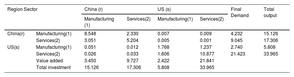
Measuring sectoral irregularities in China and the USOur data sources include the latest Multi-Regional Input–Output (MRIO) tables for 2023 from the Asian Development Bank (https://kidb.adb.org/globalization/current). Input–output data for China and the US are obtained using the original table, based on which, referencing the corresponding table of MRIO industry classification published by the Bank of Asia (https://kidb.adb.org/globalization/current), we merged industries in C3–C16 categories, classified as manufacturing industries, and industries in C19–C35 category are grouped as service industries. We then construct input–output tables for the two sectors in China and the US as the baseline data prior to trade shocks. We obtain import and export data for China and the US in 2022 and 2023 from the US–China Business Council (https://www.uschina.org/articles/us-exports-to-china-2025/)as the baseline data for trade demand shocks to calculate the initial China–US circumstances. Table 1 presents the dynamic evolution of manufacturing and service industries’ inoperability in the US and China and associated economic loss using regional input–output tables and US–China trade data.
Bi-regional Input–Output Tables for the US and China (2023, $ billion).
Initial demand perturbation is a prerequisite for assessing industrial chain resilience, wherein an economy encounters a trade shock at a specific point in time. This shock arises from a shift in demand that causes an imbalance between imports and exports on both sides of trade, which disrupts the assumed equilibrium of normal input–output supply and demand. The central aspect of simulating demand shocks in this study is to assess how initial demand fluctuations affect the economic system’s degree of inoperability, assuming that aggregate output remains constant. Table 2 details the changes in import trade between China and the US for 2022 and 2023, which we use to simulate the initial demand shocks for both countries following tariff increases. We calculate these shocks using the following formula: Industryimportvaluein2022−Industryimportvaluein2023Industryimportvaluein2022, and each industry’s initial demand perturbation is calculated as follows: C0=(0.0170.0200.0610.080)T.
Inoperability analysisInoperability measures the degree to which an infrastructure or industry sector deviates from its planned functionality following a trade shock, which is a key indicator of industrial chain resilience. The recovery cycle denotes the time required for the chain to adapt to a new supply and demand structure and return to normal operations after a trade shock. Baier and Bergstrand (2007) indicated that the economic adjustment period following a trade policy shock typically spans 6 to 12 months. During the 2018–2019 US–China trade conflict, tariff changes shifted China’s export commodity strategies, with an average recovery time of approximately one year before stabilization.
The previous analysis indicates that the degree of industrial inoperability following a trade shock exhibits an exponential decline. Therefore, we define the industrial chain recovery cycle as one year, with T = 365 days. To observe the evolution of industrial chain inoperability throughout the recovery process more comprehensively, we divide the cycle into three phases, covering t = 90, t = 180, and t = 365. Additionally, industrial chain adjustment is closely linked to the recovery rate, which depends on factors such as recovery time, recovery state, and the initial disturbance, as noted earlier.
China’s manufacturing sector is a significant proportion of the global supply chain; however, its adjustment rate is constrained by reliance on export markets and complex industrial chains. In contrast, China’s service sector is more localized (e.g., logistics and retail), which is less impacted by international trade and recovers more quickly. The US manufacturing sector relies heavily on imports from China and other Asian countries, which makes it more vulnerable to supply chain disruptions and results in a longer adjustment cycle. However, the US benefits from stronger technology and capital investments, which facilitate a certain degree of recovery. In contrast, the US service sector, which constitutes a larger proportion of the nation’s GDP, is more flexible (e.g., financial and IT services), less affected by trade, and experiences a shorter recovery cycle, bolstered by a large domestic consumer market that drives recovery.
To simplify the calculation process and facilitate the comparison of recovery rates across sectors, we set the recovery rates for the manufacturing and service industries in China and the US as k1r=0.06,k2r=0.09,k1s=0.05,andk2s=0.08. These values are used to simulate the dynamic evolution of various sectors’ inoperability in both countries.
Fig. 1 illustrates the variations in inoperability across sectors in China and the US following a trade demand shock. China’s manufacturing sector experiences an initial rise in inoperability, reaching approximately 0.045 at t = 90 days, and stabilizes at 0.05 by t = 114 days, attaining equilibrium. The sector exhibits a substantial initial shock and rapid rise in inoperability, after which the growth rate flattens, reflecting the industry’s instability. In contrast, the service sector’s inoperability increases more gradually, reaching around 0.04 at t = 90 days, which is significantly lower than that of the manufacturing sector. By t = 76 days, the service sector’s inoperability stabilizes at approximately 0.035, reaching equilibrium. The service sector exhibits smaller effects, slower inoperability growth, and lower long-term stability. The shaded region reveals that the service sector’s cumulative inoperability is much lower than that of the manufacturing sector, indicating that this sector contributes less to industrial chain fluctuations. To evaluate the robustness of the model under parameter uncertainty, we conduct a sensitivity analysis using Monte Carlo simulations. The results and associated confidence intervals presented in the Fig. 1 demonstrate that the qualitative behavior of the model and its equilibrium points remain consistent across simulations. This indicates that the model is robust to moderate variations in parameter values. Overall, this analysis confirms that our results remain robust in the presence of parameter uncertainty, supporting the stability and validity of the proposed model.

For the US, the inoperability in the manufacturing sector stabilizes at 0.12 by t = 122 days, reaching equilibrium. The manufacturing sector in the US experiences larger initial shocks but smaller subsequent growth, indicating greater overall stability. In contrast, the inoperability in the US service sector rises to 0.12 by t = 90 days, which is significantly higher than that observed in China during the same period. The inoperability in the US service sector stabilizes at 0.12 by t = 92 days, reaching its equilibrium point. The US service sector exhibits a rapid initial response, with long-term performance similar to that of the manufacturing sector’s inoperability, reflecting the US economy’s high dependence on services.
In conclusion, China’s economic shocks are predominantly concentrated in the manufacturing sector, with the highest degree of inoperability at 0.055, which is considerably higher than the 0.04 observed for the service sector. This indicates that the manufacturing sector is the primary source of economic fluctuations in China. In contrast, the inoperability in manufacturing and service sectors in the US is comparable, stabilizing at 0.12. However, the service sector shows slightly higher sensitivity to demand shocks than the manufacturing sector. Therefore, China should focus on enhancing its manufacturing sector’s risk resilience and gradually increase the share of the service sector to optimize its economic structure. Furthermore, the US should prioritize strengthening its service sector’s stability to reduce the amplifying impact on economic fluctuations.
Economic loss analysisThe cumulative economic loss formula for each industry sector i is as follows:
where x^i denotes industry i’s expected output when it is undisturbed, and Qi(t) denotes sector i’s cumulative economic loss up to time t.
Fig. 2 illustrates the dynamic trend of economic loss over time, divided by sector for China and the US. Regarding the scale of economic loss, China’s manufacturing sector experienced a gradual upward trend, reaching approximately $82 million. In contrast, China’s service sector incurred lower economic loss, with growth slowing over time and ultimately stabilizing at around $73 million. Economic loss in the US manufacturing sector increased at a faster pace, peaking at around $74 million. However, the US service sector experienced the largest economic loss, exhibiting a rapid growth phase reaching more than $430 million, followed by stabilization.

In terms of dynamic trends, in the initial period (0–50 days), economic loss increased rapidly in all sectors, with the most significant rise observed in the US service sector, followed by the Chinese manufacturing sector. In the middle period (50–200 days), the growth of economic loss across all sectors slowed considerably, and the curves gradually leveled off, with China’s service sector exhibiting the slowest growth and consistently remaining at the lowest level. In the later period (200–365 days), economic loss stabilized in all sectors, with the US service sector maintaining the highest level, while the Chinese service sector remained at the lowest level.
Overall, China’s economic loss was primarily driven by the manufacturing sector, with a smaller impact on the service sector. This is closely associated with the relatively high share of manufacturing in China’s GDP and its significant role in international trade. In contrast, economic loss in the US was primarily concentrated in the service sector, with loss in this sector far surpassing those in manufacturing. This reflects the service-oriented economic structure in the US and the amplifying effect of external shocks. Considering this, China should focus on enhancing its manufacturing sector’s risk resilience and promoting service sector growth to diversify economic risks. Furthermore, the US should work to strengthen its service sector’s stability, improve contingency planning, and reduce the amplifying impact of the sector amid overall economic shocks.
Decision space for industrial Chain’s static toughnessThe industrial chain’s static resilience decision space comprehensively integrates resilience indicators that combine initial perturbation and inoperability levels with the industrial sector’s investment function. This framework can effectively guide the development of sectoral recovery investment plans in the context of trade shocks. This section further analyzes industrial chains’ static toughness based on the previous analysis using the regional input–output data for the two sectors in China and the US as presented in Table 1. The primary intent of this section is to explore how to effectively plan for the recovery costs associated with industrial chain toughness following economic loss induced by demand shocks to facilitate rapid recovery and industrial chain stabilization.
We calculated the matrix using the data in Table 1 as follows: D*=[I−A*]−1=[2.52530.55630.00180.00280.63691.57050.00050.00090.03590.00620.01300.00381.46880.46010.10221.5031]. Due to the impact of the trade war, which results in a decline in final consumption in both countries, we assume that the maximum demand perturbation to the industrial sectors in China and the US is the same, Cmax*=[0.30.30.30.3], and that the investment function for each industrial sector is f(βi)=e−βi, where in keeping with the previous analyses, βi denotes the amount of investment required to bring the system to equilibrium between supply and demand. β1 and β2 represent the respective amount of investment in China’s manufacturing and service sectors, and β3 and β4 represent the respective amount of investment in the US manufacturing and service sectors. This can be obtained by using equation (12) as follows:

Using the above results, we obtain the weights representing the impact of investment amounts on industrial chain resilience in different industries in China and the US. We calculate each industry’s investment sensitivity by applying partial derivatives to the investment coefficients of the industrial sectors, which yields the following:

Specifically, the resilience of Chinese manufacturing is more sensitive to US services investment (0.0009) than US manufacturing investment (0.0006). The Chinese service sector’s resilience is more sensitive to US services investment (0.0004) than US manufacturing investment (0.0002). The resilience of US manufacturing is more sensitive to Chinese manufacturing investment (0.0182) than Chinese service sector investment (0.0066). Similarly, US services exhibit a higher sensitivity to Chinese manufacturing investment (0.0038) than Chinese services investment (0.0024). These results indicate that China’s manufacturing investment has a greater impact on the US industrial chain’s resilience, while the US primarily influences China’s industrial chain resilience through service sector investment.
To better illustrate the impact of different investment amounts on industrial sectors’ static resilience, we plot response curves for each industry to clarify the influence of investment strategies on industrial chain resilience and recovery.
Regarding the investment function, the exponential decay form is supported by the typical diminishing marginal returns observed in resilience investments (Sheffi & Rice, 2005). This is consistent with previous studies demonstrating that the marginal benefit of additional investment in resilience measures tends to decrease as initial vulnerabilities are addressed (Blackhurst et al. 2011). Therefore, the selected function reflects previous empirical evidence and theoretical expectations regarding resilience capacity saturation.
The results in Fig. 3 indicate significant cross-country and cross-sector differences in resilience responses. From the cross-sectional analysis, For China’s manufacturing sector (R1r), the sensitivity to parameter β1 is the highest, revealing that as β1 increases, R1r rises rapidly and eventually converges to 1, while the impact of parameters β2, β3, and β4 are negligible. Resilience in China’s service sector (R2r) is most sensitive to β2, with minimal effects from other parameters.

In contrast, the US manufacturing sector (R1s) has the strongest response to β3, and the US service sector (R2s) responds most significantly to β4. These sector-specific response curves confirm that targeted domestic investments can have a dominant effect on improving resilience compared with other parameter variations.
From a vertical comparative perspective, the results reveal that the investment parameters β1 and β2 have the greatest impact on the resilience of China’s manufacturing and service industries, respectively. Conversely, investment parameters β3 and β4 are most influential in enhancing the resilience of US respective manufacturing and service industries. This demonstrates that targeted investments in each country’s own industries are more effective in improving industrial chains’ resilience. Although these investments may have spillover effects that support the resilience of related industrial chains, their impact is less pronounced compared with the recovery effects of direct investments in the respective domestic industries.
To further examine these interactions, we fix China’s investment levels (β1 = β2 = 1) and vary US investment portfolios (β3, β4). As shown in Table 3, this scenario highlights how different US investment combinations influence the static resilience Chinese and US industrial chains. These portfolio analyses provide an empirical basis for identifying cost-effective investment mixes that balance direct domestic recovery effects with feasible cross-national spillovers.
Table 3 illustrates the impact of various combinations of US investment in manufacturing and services on China’s industrial chain, with fixed investments in China’s manufacturing and service sectors. The results comparing Plans A and B reveal that when US investment in the service sector remains constant and investment in US manufacturing rises, China’s manufacturing sector resilience improves slightly, while that of China’s service sector remains unchanged. In contrast, comparing Plans B and C, with US investment in manufacturing held constant and investment in the US service sector increased, China’s manufacturing and service sectors show improved resilience. Finally, comparing Plans A and C, where both US manufacturing and service investments rise, the resilience of both China’s manufacturing and service sectors improves accordingly.
Fig. 4 illustrates the impact of a fixed Chinese investment portfolio on US industrial chain resilience. When parameters β1 and β2 are fixed, increasing parameter β3 significantly enhances the US manufacturing sector’s toughness more than the service sector, while β4 remains constant. Conversely, when β3 is held constant and β4 is increased, the US service sector’s resilience improves more than the manufacturing sector, although the overall increase remains lower than that observed for manufacturing. These findings indicate that investments in US manufacturing are more likely to facilitate overall industrial chain resilience and recovery. The results of this sensitivity analysis indicate that different investment portfolio strategies have varying impacts on industrial chain recovery and resilience.

We next analyze the impact of China’s investment in different industries (β1, β2) on each industrial sector by fixing the amount of investment in US industries, setting β3 = β4 = 1, as shown in Table 4.
Table 4 illustrates the impact of different combinations of Chinese investment in manufacturing and services on the US industrial chain, with US manufacturing and service sector investments held constant. The results reveal that US manufacturing and service sector resilience increase when China’s manufacturing sector investment rises, while investment in China’s service sector remains unchanged (comparing Plans A and B). Similarly, when investment in China’s service sector increases while manufacturing investment remains the same (comparing Plans B and C), US manufacturing and service sectors’ toughness also improves, although the increase is smaller than that observed with higher investment in China’s manufacturing sector. Furthermore, when China’s manufacturing and service sector investments are increased (comparing Plans A and C), the resilience of the US manufacturing and service sectors improves minimally. These results indicate that investment in China’s manufacturing sector has a more significant impact on enhancing US industrial chain toughness than investment in China’s service sector.
Fig. 5 illustrates the impact of fixing the US investment portfolio on the resilience of China’s industrial chain. Comparing Scenarios A and B reveals that, with β2 held constant, increasing β1 results in significantly greater improvement in China’s manufacturing sector resilience compared with its service sector. Conversely, when β1 is fixed and β2 is increased, service sector resilience improves more than that of the manufacturing sector. However, across these three investment scenarios, the effect on promoting resilience recovery in US manufacturing and service sectors is more limited.

To further explore the optimal investment portfolio scenarios for resilience recovery in China and the US, we next conduct a numerical simulation analysis. To do so, we set the total investment for each industry sector at $500 million (βi∈[0,5]) and use an optimization algorithm to determine the optimal investment scenario to maximize each sector’s static resilience (Table 5).
Table 5 reveals the optimal investment portfolios required by China and the US to achieve maximum static toughness in manufacturing and service sectors. To reach 99 % static resilience in each sector, China requires a total investment of $3.821 billion, which is lower than the US, which requires $4 billion.
Considering each country, when China’s service sector reaches 99 % static toughness, the required investment is $1.826 billion, compared with $399 million and $427 million for the US manufacturing and service sectors, respectively. When China’s manufacturing sector reaches 99 % resilience, the required investment rises to $1.995 billion, with $495 million and $500 million invested in US manufacturing and service sectors, respectively. This indicates that achieving the same level of toughness in the service sector is less costly than in the manufacturing sector with China’s investment unchanged. In contrast, for the US, regardless of whether it is the manufacturing or service sector reaching 99 % static toughness, the required investment is around $500 million, totaling $2 billion.
We draw the following conclusions from this comparative analysis. When both countries achieve the same maximum level of static toughness in their industrial sectors, the US requires significantly more investment than China. Specifically, China has lower investment needs, particularly in the service sector, where it demonstrates greater flexibility and resilience. Conversely, the US is more reliant on external investment to withstand shocks and restore industrial resilience.
Overall, when faced with the same demand shock, China’s industrial sector requires less investment than the US to achieve the same degree of recovery, indicating stronger resilience in China’s industrial chain. Therefore, investment in China’s manufacturing and service sectors is more cost-effective than investment in the US, providing a more efficient route to improving resilience in both countries. Notably, investment in China’s manufacturing sector has a more significant impact on resilience than service sector investment.
Industrial Chain dynamic toughness decision spaceWe build upon the static decision framework by incorporating recovery time to construct the dynamic resilience decision space for industrial chains. This approach constructs a dynamic decision model comprising resilience indicators such as normality, recovery time, and initial disturbance to evaluate the effectiveness of these indicators in addressing trade shock decisions. We designed two scenarios (Table 6) for comparative analysis based on the input–output data in Table 1. Plan A requires that each industry recover to 96 % of its initial level (FA=0.96) when facing the maximum external shock qm=0.4 = 0.4, and Plan B requires a recovery to 98 % (FB=0.98) at the same maximum external shock qm=0.4. Assuming that all sectors recover 90 % of the maximum external shock at equilibrium (ri=0.9), the constant is calculated on the basis of equation (18): Li=2.30.
Using equation (15), the dynamic toughness decision portfolio of the industrial chain under the two scenarios, Fi,τi,and qim can be obtained as follows:


Through a quantitative analysis of the distribution characteristics of dynamic toughness (Fig. 6), we compare the dynamic toughness performance of two different recovery objectives (FA and FB) under the same maximum perturbation intensity of qm=0.40. The results indicate that the recovery objective choice significantly influences industrial toughness, even under the same external shock intensity.

Specifically, when industries are subjected to 40 % of the maximum external shock, scenarios FA (25.56, 0.40) and FB (12.78, 0.40) correspond to recovering 96 % and 98 % of the original level, respectively. The results reveal that the resilience characteristics under the two scenarios are heterogeneous. Under the same perturbation intensity, Plan B’s recovery period (τi), which recovers to 98 %, is about 50 % of that of Plan A, which recovers to 96 %. This indicates that higher resource inputs can significantly enhance industrial chain resilience to shocks and improve recovery efficiency, and the time required for an industry to recover exhibits a trend of marginal incrementality.
Fig. 6 analyzes the dynamic evolution of industrial resilience, reflecting two notable impacts from different scenarios on industrial resilience. First, by increasing resource inputs under the condition of no strict resource constraints, Plan B enables the industry to recover to 98 % of its original level within a relatively short recovery cycle (12.78 days) when facing a 40 % shock, demonstrating excellent resilience and rapid recovery characteristics. Second, under obvious resource constraints, Plan A adopts a more conservative resource allocation strategy, and although the recovery cycle is relatively long (25.56 days), it is still able to restore the industry to 96 % of its original level under the same perturbation, demonstrating high resource use efficiency. This differential resilience performance provides a basis for decision makers to choose the optimal solution under different resource constraints.
For policymakers, if cost is not a consideration, Option B should be chosen to achieve a higher recovery level in a shorter period of time and enhance the industry’s resilience to shocks and rapid recovery. However, in the case of limited resources, Plan A is a more reasonable choice, with a final level of recovery that does not differ considerably from that of option B, despite the longer recovery time. This comparison provides a valuable reference for policymakers to optimize industrial investment strategies under different economic and resource environments, thereby enhancing overall industrial chain resilience and stability.
To further compare the dynamic resilience of each industrial sector in China and the US and the effects of different decision-making options, we conduct an analysis of the dynamic resilience decisions for each sector. The conditions are that the recovery period of each sector remains the same, T1=T2=T3=T4=100 days, and the maximum disturbance encountered is also the same q1m=q2m=q3m=q4m=0.4. Substituting the data in Table 1 into equation (16), we compute the decision space for the following dynamic resilience index of each sector, F=g(qm,τ,K):

According to the previous analysis, formula kii(1−∑j=1naij*)τi=Li describes the relationship between the recovery rate and the recovery time in each sector, where aij* is the diagonal matrix element of A*, and can be substituted into the data in Table 1 to obtain the relationship between recovery rate kii and recovery time τi in each sector: {0.28k1rτ1=2.300.52k2rτ2=2.300.47k1sτ3=2.300.63k2sτ4=2.30
We demonstrate the relationships between the mean normal level (F), recovery rate (K), and recovery time (τ) by constructing contour plots for each sector. These plots illustrate the dynamic resilience of each sector under different combinations of parameters for a given shock.
Fig. 7 illustrates the changes in industry resilience response under different investment portfolios, where the k value, which measures the recovery rate, is closely related to the investment level. Comparing the performance of the curves of China and the US in manufacturing and services sectors reveals significant differences in recovery rates and resilience between China and US industries. Specifically, the analysis shows that China’s manufacturing sector has a higher recovery rate (larger k value) in a shorter recovery time (lower τ value), indicating more short-term resilient. However, as the recovery time lengthens, the k value gradually declines, reflecting weakening long-term resilience. This means that short-term gains for China’s manufacturing are substantial, but the marginal effect diminishes over time, indicating that continuous investment is needed to sustain resilience. In contrast, the recovery rate curve for China’s service sector has a lower but more stable k value, indicating that although the initial recovery is slower, its resilience remains stable over time. This demonstrates a smaller immediate effect but larger long-term cumulative effects, which is relevant for sectors such as digital and financial services that require sustained stability.

The US manufacturing sector also demonstrates a high short-term recovery rate, although its recovery rate gradually slows down over time, reflecting moderate long-term stability. This indicates that while investment can significantly boost US manufacturing recovery in the early stages, strategic reinvestment is required to maintain resilience. In contrast, the US service sector has a lower initial recovery rate and strong long-term resilience, and the k value remains stable. This indicates that even modest increases in investment can yield enduring resilience benefits, particularly for knowledge-intensive industries. These sector-specific patterns clarify that the magnitude of k changes translates into practical differences in recovery speed and stability, directly informing policymakers how to prioritize investment portfolios. For example, China’s manufacturing should balance short-term recovery boosts with long-term sustainability, while the US service sector should leverage its inherent stability through progressive investment scaling. This provides a significant reference for designing targeted investments and cross-border cooperation strategies to build more resilient industrial chains under external shocks.
Plans A and B in Table 7 provide strong support for specific values of industry resilience under different portfolios. In Plan A, the lower recovery rate (0.322 for Chinese manufacturing) and longer recovery period (about 25.5 days) indicate that this scenario improves long-term resilience and is suitable for scenarios that require stable recovery. In contrast, Plan B enables the industry to achieve short-term recovery more quickly through higher recovery rates (0.645 for Chinese manufacturing) and shorter recovery periods (about 12.75 days). However, this high investment intensity is also accompanied by higher volatility and risk, while enabling an accelerated recovery.
Combining the results from Fig. 7 and Table 7 indicates that industry resilience varies across different investment portfolios. Overall, the services sector demonstrates stronger resilience in China and the US, particularly in terms of long-term recovery, where it shows higher stability. In contrast, manufacturing sector resilience is more sensitive to investment intensity, in which increased investment boosts short-term recovery and may slightly affect long-term stability.
This analysis indicates a clear trade-off between short- and long-term resilience in the industrial chains of the US and China, depending on the chosen investment portfolios. The service sector tends to exhibit greater stability in terms of long-term resilience enhancement, which is practically significant for policy design intended to sustain growth during prolonged external shocks. This means that policymakers should prioritize steady investments in the service sector to maintain high resilience over time. Conversely, manufacturing sector resilience requires sufficient upfront capital and sustained reinvestment to maximize immediate recovery and longer-term stability. In practice, this implies that short-term stimulus alone is insufficient, and a phased investment strategy is crucial for maintaining competitiveness and supply chain security.
ConclusionsThis study examines comprehensively examines the industrial chains of China and the US, quantitatively assessing the economic loss recovery cycles and resilience dynamics from trade demand shocks. Developing a risk identification–resilience evolution–cost recovery risk management framework, this study clarifies how different industrial chain configurations influence their ability to withstand and recover from external shocks. The findings reveal significant differences in recovery patterns and the influence of targeted investments on enhancing sectoral resilience.
For China’s manufacturing sector, which has experienced substantial economic loss and relatively slow recovery, strengthening resilience should focus on investments in advanced, green, and smart manufacturing technologies, supply chain diversification, and reducing reliance on external markets. Accelerating digital transformation and establishing robust risk management systems will further enhance the sector’s ability to navigate demand fluctuations and uncertainty. For the US service sector, which is highly sensitive to demand shocks, resilience enhancement should prioritize digital economy, finance, and healthcare investments, coupled with effective risk management mechanisms. Promoting innovation and digital transformation in the service sector will increase the sector’s stability and strengthen its position in the global supply chain. This study also reveals that cross-border investment between the two countries has a mutually reinforcing effect on resilience. Investment in China’s manufacturing supports the US industrial chain’s stability, while US investment in China’s service sector boosts China’s resilience. Deepening complementary investment cooperation by expanding advanced manufacturing, green technologies, and digital infrastructure in China and supporting financial technology, information services, and education in China’s service sector can mitigate external economic shocks and reduce global supply chain uncertainty.
Research contributionsTheoretically, this study extends risk management and resilience theory by demonstrating how static and dynamic resilience indicators can be operationalized and embedded within a decision space framework that emphasizes the integrated treatment of risk identification, resilience evolution, and cost recovery. The results demonstrate how the proposed model bridges static and dynamic resilience dimensions, responding directly to the identified research gap in which existing models often treat risk and resilience independently. Compared with existing static input–output models (Dormady et al. 2019) that predominantly assess one-time impact and recovery, our approach captures the evolution of resilience over multiple recovery cycles, which is consistent with dynamic modeling perspectives such as those discussed by Ivanov and Dolgui (2020). Moreover, unlike conventional resilience assessments that often treat risk and resilience independently (Hosseini et al. 2020), this study demonstrates how these two dimensions interact through investment sensitivity pathways. Furthermore, the use of sector-specific decision spaces extends the work of Wieland and Wallenburg (2013).
Practically, the proposed framework enables forward-looking dynamic risk management by incorporating resilience metrics into investment decisions. This approach provides managers with a useful quantitative decision-making tool to guide industrial chains’ recovery, ensure long-term stability, and foster organizational learning to mitigate risks in future projects. At the same time, policymakers must consider the feasibility of achieving carbon emissions improvements while maintaining cost-effectiveness (Liu & Liu. 2023; Zhu & Zhang. 2023). Balancing investments in green technologies with immediate economic priorities may require phased implementation and careful assessment of resource allocation tradeoffs. This perspective ensures that resilience-building measures are not only technically sound but also practically viable in the context of China’s broader industrial and sustainability goals.
Moreover, the model’s potential global applicability extends its relevance beyond the US–China context. By demonstrating how targeted investments and cross-border cooperation can mutually reinforce industrial resilience, the framework offers practical insights for policymakers developing economic cooperation or trade policies under high uncertainty. This global perspective highlights the model’s value in guiding risk-sharing arrangements and enhancing supply chain security worldwide.
Overall, by bridging theory and practice, this study provides clear guidance for building more robust, adaptable, and globally relevant industrial chains to withstand rising trade and geopolitical risks.
Limitations and future researchThis study has some room for future expansion, including the focus on the US–China context, the simplified treatment of technological change, and the absence of firm-level behavioral data. Future research could expand the model’s generalizability to other regions, incorporate digital resilience indicators, and employ multiagent simulations to capture intraindustry and firm-level dynamics more comprehensively. Such extensions would further refine and validate the framework’s global applicability and value for informing cross-border supply chain cooperation.
CRediT authorship contribution statementShangfeng Zhang: Writing – review & editing, Project administration, Funding acquisition. Shibo Xu: Writing – original draft. Duen-Huang Huang: Writing – review & editing. Zhenghao Zhang: Data curation. Yukun Zheng: Formal analysis. Can Cheng: Validation, Methodology, Data curation. Wenxiu Zheng: Data curation.
There are no conflicts of interest to declare.
This work was supported by the ZheJiang Social Science Foundation (24ZJQN117Y;26QNYC017ZD*;20NDJC335YBM), Zhejiang Soft Science Project (2025C35092), National Social Science Foundation of China (22&ZD162), Economic Forecasting and Policy Simulation Laboratory, Zhejiang Gongshang University (2024SYS026), the Fundamental Research Funds for the Provincial Universities of Zhejiang (2024ZDAPY02), the Summit Advancement Disciplines of Zhejiang Province (Zhejiang Gongshang University - Statistics), the Collaborative Innovation Center of Statistical Data Engineering Technology & Application; Zhejiang Gongshang University Graduate Research and Innovation Fund Project (ZDXM2024004), and Higher Vocational Education Research Project of Wenzhou Polytechnic (WZYGJzd201702). Thanks to the anonymous reviewers and Prof Domingo and Prof Malin Song for their valuable comments and generous help.