Making explosive cocktails: Recipes and costs of 20 Argentine crises from 1865 to 2004

Abstract

The objective of this paper is twofold. Firstly, we investigate what were the “recipes” of the 20 Argentine currency crises from 1865 to 2004 using regression tree analysis, which is a non-parametric data classification technique. Secondly, we evaluate the costs of Argentina's crises in terms of output losses and recovery time.

We obtained three “recipes” that constitute an early warning system. The most costly and frequent mix has two “ingredients”: high Public Expenditures (% of GDP) and Current Account Deficit (% of GDP). The less frequent and less costly mix consists of moderate Public Expenditures, Real Exchange Rate Overvaluation, and high International Interest Rates. Finally, the mix with intermediate costs and medium frequency is made up of five ingredients: moderate Public Expenditures, Real Exchange Rate Overvaluation, moderate International Interest Rates, strong decline in Bank Deposits, and high ratio of Monetary Aggregate M2 to International Reserves.

Resumen

Este trabajo tiene un doble objetivo. Primero investiga cuales son las “recetas” de las 20 crisis Argentinas en el periodo 1865–2004 mediante Classification Tree Analysis, una técnica de clasificación de datos no paramétrica. En segundo lugar, evalúa los costos de las crisis en términos del PBI perdido y del tiempo de recuperación.

Obtenemos tres “recetas” que constituyen un sistema de alerta temprana. La mezcla más costosa y frecuente tiene dos “ingredientes”: elevado gasto público (% del PBI) y déficit de cuenta corriente (% del PBI). La mezcla menos frecuente y menos costosa se hace con Gasto público moderado, sobrevaluación del tipo de cambio real y elevadas tasas de interés internacional. Por último, la mezcla con costos y frecuencia intermedia tiene cinco ingredientes: Gasto público moderado, sobrevaluación del tipo de cambio real y tasas de interés internacionales moderadas, fuerte caída en los depósitos bancarios y elevado ratio del agregado monetario M2 a reservas internacionales.

1

Introduction

Major economic phenomena usually revive the interest of scholars in studying similar events in the past. The Eurozone crisis has not been the exception. Its deleterious effects on output and employment have spurred a myriad of papers that dig into the history for lessons to understand the present. Some researchers have focused their attention on specific crisis such as the Great Depression, while others have concentrated on particular sets of crises covering countries from several geographic regions and different historical periods. In this paper, we propose a different approach. We look into the past of a single country, covering most of its history in an attempt to embed our findings within a broader empirical and theoretical debate regarding crises “ingredients” around the globe.

Is there any country with such a useful past that deserves special attention? We claim that Argentina is one the most interesting cases to study. Its record includes 24 crises from 1823 to 2002 (Cerro and Meloni, 2003, 2013), which implies 50 crisis years when counting long-lasting episodes. That is, one crisis every seven and a half years and one crisis year every three and a half years, more than any other country in the world (Eichengreen and Bordo, 2002). How does Argentina come to have such a large number of crises and crisis years? Do crises have a common “recipe” or are there a variety of potential mixtures? If so, what are the ingredients of such “explosive mixes”? Are they made with import components, such as increases in international interest rates, changes in the international capital market conditions, or declining prices on exports? Or are they also obtained with national “condiments” such as fiscal deficit, high indebtedness and real exchange rate overvaluation? How many ingredients are needed to make an explosive cocktail? Furthermore, which is the most expensive mix?

To answer these questions, we investigated the “recipes” of the 20 currency crises suffered by Argentina from 1865 to 2004 by means of a Classification Tree Analysis (CTA), a non-parametric data classification technique widely used in several disciplines for early detection of distress events. The application of a Classification Tree Analysis to the economics of the crises field was pioneered by Kaminsky (2006) who identified six varieties of crises from a sample of twenty countries for a large period starting in the 1970s. This technique arose as an alternative to parametric approaches, including logit and VAR models, and also non-parametric, such as the leading indicators methodology. Our inputs were the 20 financial crises identified by Cerro and Meloni (2003, 2013) and fourteen financial and macroeconomic variables suggested by the theoretical and empirical literature (Frankel and Wei, 2004; Kaminsky, 2006). We looked for an early warning system that would help to anticipate crises. Economic historians have studied extensively the case of Argentina, focusing on specific crisis or sets of crises in particular historical periods (Cortés Conde, 1989; Choueiri and Kaminsky, 1999; della Paolera and Taylor, 1999, 2000; Bordo and Vegh, 2002). Our approach was to aim at complementing their findings.

We have also evaluated Argentina's crises’ costs in terms of output losses and recovery time. We carried out a variant of the International Monetary Fund (IMF, 1998) methodology that entails the computation of cumulative output loss relative to trend.

This paper is organized in four sections. In the following section we summarize the methodology to identify crises for a time span of 139 years and highlight some features of the main crises. In Section 3 we identify the ingredients of “explosive mixes” by means of the CTA Method, and in Section 4 we evaluate the costs of currency crisis in terms of output losses and recovery time. Section VI carries our concluding remarks.

2

Argentine crises

The literature on the Argentine economic history shows considerable agreement about the identification of the most significant Argentine crises. The episodes of 1826–1827, 1838–1840, 1845–1848, 1890, 1929/1930, 1976, the turbulent 1980s, and the latest 2001/2002 are unanimously rated as crises by the majority of scholars. Similarly, other events, such as the ones in 1876, 1884 1914, 1948–1949, 1959, 1964, and 1971, also have great consensus about their qualification as crises. However, for a long time this agreement was rather loose, lacking a precise definition of crisis and hence about the variables to look at when describing a crisis. A standard way to identify currency crises is through the Market Turbulent Index (MTI) defined as the sum of three components: the rates of change of international reserves, exchange rate, and interest rate, weighted by the inverse of the respective standard deviation to avoid having the most variable component dominate the index movements.¹ In this framework, currency crises are defined as situations in which speculative attacks on the exchange value of the currency result in a devaluation (or sharp depreciation) of the currency, a rapid decrease in international reserves, an abrupt increase in interest rates, or some combination of these.²

This is the approach followed by Cerro and Meloni (2003, 2013) to identify crises in Argentina from 1823 to 2003.³ They constructed an MTI for six sub-periods: 1825–1861 (from the President Rivadavia administration to the National Organization, President Mitre administration); 1862–1913 (from the Mitre administration to World War I); 1914–1945 (from World War I to World War II); 1946–1975 (from the first to the third President Perón administrations); 1976–1991 (from the first to the second hyperinflation); and 1992–2002 (convertibility years). Depending on how large the deviation was from the MTI mean, Cerro and Meloni classified crises as very deep (or crashes), deep, or mild. Their emphasis was on crises. But since we stress “crisis year” instead of “crisis,” using their data set, we recomputed MTI and redefined crises and crisis year to capture minor turbulences that usually precede a crisis because we are interested in constructing an early warning system. If the actual MTI was greater than half of the standard deviation (computed for each sub-period) for three consecutive months, we classified that year as a crisis year.

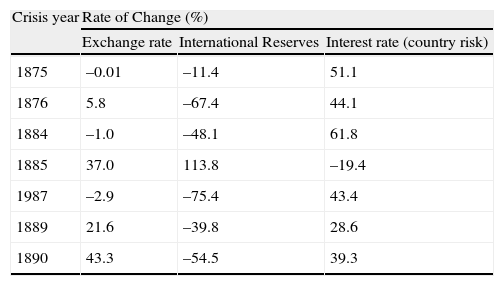
Table 1, Panels A and B, shows the behavior of the MTI and its components for each crisis year for the periods of 1865–1913 (calculated from annual data) and of 1914–2002 (calculated from monthly data). Computations from annual data might have resulted in an underestimation of the number of crisis years since episodes within a given year cannot be detected by the index duration. Due to data availability, the MTI only includes the variable exchange rate from 1865 to 1874.

Table 1.

Panel A. Crises Years characteristics: 1865-1913. Computed from Annual data.

Crisis year	Rate of Change (%)
	Exchange rate	International Reserves	Interest rate (country risk)
1875	–0.01	–11.4	51.1
1876	5.8	–67.4	44.1
1884	–1.0	–48.1	61.8
1885	37.0	113.8	–19.4
1987	–2.9	–75.4	43.4
1889	21.6	–39.8	28.6
1890	43.3	–54.5	39.3

Panel B. Crisis Years characteristics: 1914-2003. Computed from Monthly data
Crisis year	Rate of Change (%)
	Exchange Rate	International Reserves	Interest Rate
1914	0.6	–15.4	16.7
1919	4.0	2.6	23.1
1920	26.1	19.4	–7.8
1921	4.5	0.0	6.6
1929	3.0	–16.5	24.0
1930	21.1	7.1	–14.2
1931	33.6	–36.4	8.2
1937	3.5	–0.5	1.7
1938	28.6	–0.7	5.6
1948	131.6	–35.1	na
1949	76.5	–14.1	na
1951	90.3	–28.5	na
1958	97.3	–55.8	na
1962	77.9	–64.6	na
1964	47.3	–52.4	na
1965	8.8	–23.5	na
1971	134.1	–63.6	13.3
1972	40.6	–24.0	33.8
1975	537.7	–59.6	165.9
1976	112.6	–15.9	43.0
1981	454.4	–34.1	92.2
1982	567.1	–25.3	65.9
1983	254.9	–65.5	62.9
1985	256.3	187.5	–74.3
1986	81.8	–42.4	73.8
1987	167.0	–45.8	279.4
1988	188.5	140.1	77.1
1989	7729.1	–36.7	114.9
1990	260.3	235.8	28.5
1991	51.8	–28.4	37.5
1994	0.3	–16.6	20.4
1995	–0.5	–28.1	76.5
1998	0.1	–11.1	35.8
2000	0.1	–10.9	66.2
2001	3.5	–39.4	339.9
2002	114.7	–53.5	252.0

Notes: Rates of change of exchange rates, international reserves and interest rates were computed from peak to trough.

Source: own calculations based on Cerro and Meloni (2003, 2013).

2.1

Major crises in the 19th century

Before the National Organization period (starting in 1862), most of the crises were associated with international conflicts that resulted in blockades to the port of Buenos Aires and hence in dramatic falls in the revenues from import tariffs, the main source of financing the public budget, which in turn was high and growing due to military spending. The country suffered three blockades: the first one, in 1826, during the war against Brazil (1825–1827); and then two more: in 1838–1840, performed by the French; and in 1845–1848, carried out by the combined French and British forces.

On the other hand, the three episodes dated in the last quarter of the century, the crises of 1876, 1885 and 1889/1891, were good examples of inconsistency between monetary and fiscal policies (see Fig. 1). During the Sarmiento administration (1868–1874), expenditures had grown considerably not only because the war with Paraguay and various conflicts in the provinces demanded military outlays but also due to the ambitious public investments plan.⁴ Argentina had a convertibility regime, and the adverse international conditions that started in 1873 led to a contraction in the gold-backed money supply, forcing the government to sell the stock of metallic notes and to reduce public-sector expenditures. The attempts to sterilize the negative effects of gold outflows failed and finally convertibility was abandoned in May 1876,⁵ with a consequent devaluation of the currency.

Fig. 1.

Domestic Inconsistencies in the 19th Century Crises.

Source: Own calculations based on Ferreres (2005).

The crisis of 1885 had similar features. By July 1883 the paper-peso exchanged at par with the gold-peso.⁶ The period of convertibility lasted only seventeen months. By the end of December 1884, the banks of issue did not stand ready to sell gold at par to all who offered the metallic note. Hence, in March 1885 the federal government decreed the inconvertibility of paper money.

The 1889/1891 crisis was one of the deepest in Argentine history. The root of the crisis can be found in the poor administration of President Juárez Celman, which was characterized by an outrageous increase in public expenditure (98% in 1889) and a high level of indebtedness, both external and domestic (the ratio of debt to exports increased 89% from 1887 to 1890). In this period, the government created the National Guarantee Banks (Bancos Nacionales Garantidos); that is, banks were entitled to print their own money, which led to huge increments in the monetary base (131% in 1889). High levels of public indebtedness coupled with easy monetary policy brought about devalued expectations, with the consequent fall in specie reserves. In 1891 reserves had fallen 160% relative to 1888. In 1890 most private and public banks went broke, and, given the impossibility of facing their obligations, a generalized default was declared.

2.2

Major crises in the 20th century

The first crisis of the 20th century occurred in 1914. World War I forced President de la Plaza to suspend the full convertibility of the peso in August 1914, after 13 years under the gold standard regime.⁷ The consequences were a 10.4% drop in GDP, a 15.4% fall in International reserves and a 1.7% increase in interest rates.

After WWI, Argentina accumulated important current account surpluses with the European nations but a deficit with the new economic power: the U.S. This situation generated another crisis, though mild, when the British pound lost 25 percent of its value against the U.S. dollar in 1920–1921 (della Paolera, 1994; Díaz Alejandro, 1975).

Argentina returned to the currency board system in 1927 but abandoned it a few months later, in December 1929, compelled by an unfavorable external condition: the Wall Street Crash. Gold backing of the domestic currency diminished from 80% in 1928 to 45% in 1931, and the paper peso suffered a 65% depreciation relative to the U.S. dollar. Despite being hit hard by the international crash (GDP fell 4.1% in 1930, 6.9% in 1931 and 3.3% in 1932), Argentina was the only major Latin America debtor to honor the service on its external debt but at the cost of using about 60% of the gold reserves at the Conversion Office (della Paolera, 1994). Fig. 2 displays the behavior of the U.S. interest rate and the terms of trade from the beginning of the 20th century to the Great Depression, which is usually considered to be the end of the export-led development model and the beginning of the closed economy period. The three peaks observed in the U.S. interest rate during this lapse are associated with the crisis in 1914, 1920–1921, and 1929–1930. The influence of declining terms of trade with crises is evident in the years 1920–1921 and also in 1929, but there is no relationship with the crisis of 1914.

Fig. 2.

The role of international conditions.

Source: Own calculations based on Ferreres (2005).

Another important crisis occurred in 1948/1949 under Perón's administration, which was characterized by high intervention in the price system and strict banking credit control. Perón redistributed income toward the laborers by increasing minimum wages and controlling output prices. He obtained a rapid industrialization by altering the relative price of agricultural versus industrial goods in favor of the former. From 1946 to 1949, Perón carried out expansive fiscal and monetary policies financed by Central Bank reserves and inflation taxes. Fiscal expenditures were of such magnitude that they evaporated reserves as well as pension system funds. Anti-inflationary measures taken during 1949 and 1950 failed and the crisis reappeared in 1951.

In 1958, 1962, 1964, 1971 and 1975 there were other crisis episodes marked by failed attempts to stabilize the economy in a context of alternation between democratic and military governments. There were four coups d’ état: in 1955 (removed Perón), 1962 (removed Frondizi), 1966 (removed Illia), and 1976 (removed Martínez). The first hyperinflation took place in 1975 under María Estela Martínez de Perón’ administration and the second in 1989, after a decade full of crises characterized by a spiral of devaluation and inflation. The decades of 1970 and 1980 were characterized by an expansionary fiscal policy fueled by subsidies and state-owned enterprises’ deficits. By 1987 subsidies to private production amounted to 6.6% of the GDP, and the deficit of state-owned firms reached almost 4% of GDP. As international credit markets narrowed after the debt crisis of 1982, the only source left to finance public expenditures was money printing, which generated an out-of-control inflationary process. In 1989 the inflation rate peaked at 3079%, and in 1990 it reached 2313%. During this period there were various attempts to stabilize the economy using the exchange rate to anchor prices, which resulted in real-exchange rate appreciation, current account deficits and a decline in international reserves. Fig. 3 depicts the evolution of public expenditures and current account deficits (as a percentage of the GDP).

Fig. 3.

Evolution of public expenditures and current account deficit (% GDP): 1975–2004.

Source: Own calculations based on Ferreres (2005).

After a successful stabilization plan in 1991, Argentina finally enjoyed a decade free of inflation. In the sub-period 1991–2002, only two crises occurred in 11 years. The first one, in 1995, known as the “tequila” crisis for its roots in the Mexican devaluation of 1994, was short but deep. The second, during 2001 and 2002, fueled by expansive fiscal policy and high sovereign debt, was one of the deepest in Argentina's history.

The behavior of the variables in Table 1 Panel B deserves some comments. First, devaluations/depreciations during crises increased over time, but clearly the 1948/1949 crisis stands out for the magnitude of the devaluation, 247%, which was unusual for those years. It can also be observed that the 1975/1976 crash constitutes a hinge. Before that crisis, devaluations ranged between two-digits and the lower three-digits and from 1975/76, climbed to the four-digits, reaching a peak in the 1989/1991 crash. The smallest devaluations were those corresponding to the 1914 and 1918/1919 crises with percentages lower than 1%. Second, international reserves also show a declining trend, with percentages below 50% until 1955, and almost doubled thereafter. To illustrate the magnitudes involved in each period, notice that the 1929/1931 crash implied a 49% fall in international reserves, the largest in the first half of the century, but modest if compared to most of the mild and deep crises in the second half of the 20 century. Third, interest rates also present two periods. For the crises before 1940, the growth rate never surpassed 30% while for the crises in the last quarter of the 20th century, the three-digit rate of change was the norm. Fourth, except for the 1929/1931 crash, which lasted 22 months, the amplitude of the crises before the 1975/1976 crash only occasionally reached a year, while for the rest of the century, the amplitude was in the neighborhood of two years, with the sole exception of the commonly called Tequila Crisis in 1994, which had a four-month duration.

3

Searching for ingredients of explosive mixes

Which are the most active ingredients of the “explosive mixes” made in Argentina? To answer the question, we carried out a CTA. We used this technique to identify separately the variables involved in each crisis. The output of the CTA method is a set of terminal nodes, called a tree. Each terminal node characterizes a crisis or a group of crises. The method considers an initial split of the data into two subgroups, favoring homogeneity within each group and heterogeneity between the groups. This split is repeated in sequential form until each subset terminates either when there is no impurity reduction from splitting or when the number of observations in the cell is less than a specified number of rows (or observations). Many different criteria can be defined for selecting the best split at each node. However, the properties of the final tree selected are insensitive to the choice of the splitting rule. Variable misclassification costs and prior distributions can be incorporated into the splitting structure in a natural way.

CTA is a form of binary recursive partitioning. The term “binary” implies that each group of crises, represented by a node in a decision tree, can only be split into two groups. Thus, each node can be split into two child nodes, in which case the original node is called a parent node. The term “recursive” refers to the fact that the binary partitioning process can be applied over and over again. Thus, each parent node can give rise to two children nodes and, in turn, each of these children nodes may themselves be split, forming additional children. The term “partitioning” refers to the fact that the dataset is split into sections, or partitioned.

The CTA has several advantages over traditional statistical methods. When using CTA, researchers do not have to worry about selecting predictor variables nor about the distribution of predictor variables. CTA allows for the inclusion of several variables whether normally distributed or not, avoiding costly variable selection and transformation. CTA is also recommended over traditional statistical methods when data have complex interactions or patterns. For example, the value of one variable (e.g., GDP) may affect the importance of another variable (e.g., debt). These types of interactions are generally difficult to model and virtually impossible to model when the number of interactions and variables is large.

Before running the software Decision Tree Regression (DTREG) that performs a CTA, we chose the target and predictor variables to build the decision tree⁸:

• A.

  Target variable. Our target variable was crisis years, a dummy variable that takes the value 1 if the MTI identifies the year as a crisis year and 0 otherwise. We have 43 crisis years and 97 non-crisis years in our sample. We did not distinguish among crises intensity, i.e. very deep, deep, and mild.

• B.

  Predictor variables. We included fourteen predictor variables chosen from the prescriptions of the first, second, and third generation models of crisis and also the “Sudden Stops” theory.⁹ Our predictor variables are as follows: “Public Expenditures” (% GDP), “Fiscal Result” (%GDP), and “Debt as percentage of GDP” representing first generation models. The second generation models stressed “Real Exchange Rate Overvaluation,” “Current Account as a percentage of the GDP,” and the “Rate of Growth of GDP,” “GDP per Capita,” and “Exports and Imports.” Third generation models considered the following key variables: “Ratio of Monetary Aggregate M2 to International Reserves,” “Rate of Growth of Real Total Bank Deposits,” and “Ratio of Sovereign Debt to Exports¹⁰.” “Sudden Stop” models emphasize the role of international interest rates and Terms of Trade (TOT). All predictor variables were lagged during one period to use them as early warnings except for the rate of growth of real total banking deposits and monetary aggregate M2 to international reserves that were lagged during two periods. This inclusion of this group of variables only pretends to show where the focus of the main theories at stake is. More than testing the relevance of particular models, we looked for the recipe of crises in Argentina throughout its history¹¹.

3.1

Data sources

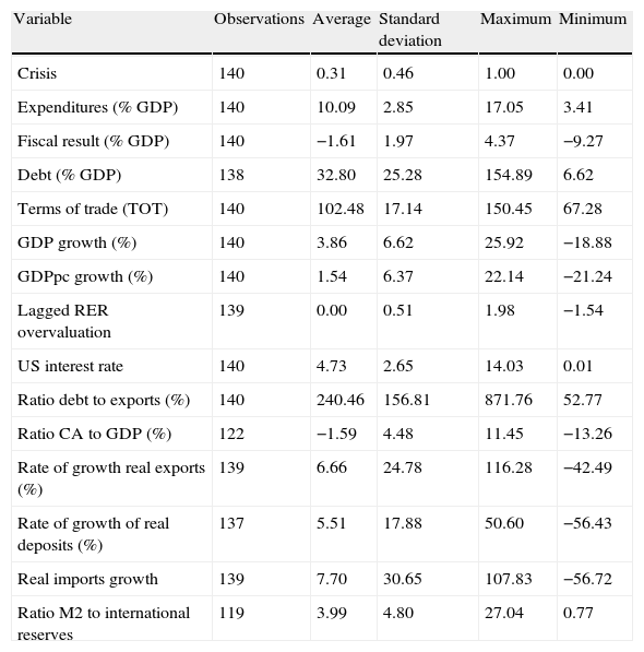
Most of the time, we took series from Dos siglos de Economía Argentina 1810–2004, the compilation of Ferreres (2005) that gathers disperse statistical information and builds long term series from diverse official sources and from several economic historians’ estimations. Table 2 provides summary statistics for each of the analyzed variables.

Table 2.

Descriptive statistics.

Variable	Observations	Average	Standard deviation	Maximum	Minimum
Crisis	140	0.31	0.46	1.00	0.00
Expenditures (% GDP)	140	10.09	2.85	17.05	3.41
Fiscal result (% GDP)	140	−1.61	1.97	4.37	−9.27
Debt (% GDP)	138	32.80	25.28	154.89	6.62
Terms of trade (TOT)	140	102.48	17.14	150.45	67.28
GDP growth (%)	140	3.86	6.62	25.92	−18.88
GDPpc growth (%)	140	1.54	6.37	22.14	−21.24
Lagged RER overvaluation	139	0.00	0.51	1.98	−1.54
US interest rate	140	4.73	2.65	14.03	0.01
Ratio debt to exports (%)	140	240.46	156.81	871.76	52.77
Ratio CA to GDP (%)	122	−1.59	4.48	11.45	−13.26
Rate of growth real exports (%)	139	6.66	24.78	116.28	−42.49
Rate of growth of real deposits (%)	137	5.51	17.88	50.60	−56.43
Real imports growth	139	7.70	30.65	107.83	−56.72
Ratio M2 to international reserves	119	3.99	4.80	27.04	0.77

Source: Own calculations based on Ferreres (2005).

3.2

Empirical results: recipes for crises

The results of the Classification Tree are reported in Fig. 4. Observations were assigned to eight terminal nodes, three characterizing crisis years and five featuring non-crisis years. Notice that the results are crisis years and not crisis. That is, a given crisis episode lasting two or three-year may have one recipe for one year and a different mix of variables for the others. The “ingredients” of each of the crisis nodes are as follows:

Fig. 4.

Classification tree results.

First mix (Node 7), Moderate public expenditures plus real exchange rate overvaluations plus high international interest rates: That is, combining unfavorable external conditions, represented by an international interest rate greater than or equal to 5.7%, with the real exchange rate overvaluation generated a currency crisis with a probability of 1 even if the government was following a rather moderate public expenditure policy (public expenditure is less than or equal to 12.2% of GDP). High international interest rates impacted not only domestic interest rates affecting investment and consumption but also debt services. We found 7 years sharing this mix of key variables: 1875, 1914, 1919, 1921, 1930, 1971 and 1991.

Second mix (Node 11), Moderate public expenditures plus real exchange rate overvaluations plus moderate international interest rates plus strong decline in real bank deposits plus an increase in the ratio of monetary aggregate M2 to international reserves: The probability of crisis when mixing these five “ingredients” was 83.3%. There were 12 crisis years in this node (1876, 1887, 1929, 1931, 1937, 1938, 1948, 1964, 1965 and 1972) but two of them (1882 and 1961) were misclassified.

Third mix (Node 16), High public expenditures (% of GDP) plus current account deficit (% of GDP): The probability of crisis when mixing these two ingredients was 77.3%. There were 17 crisis years correctly classified in this node: 1890, 1962, 1976, 1981, 1982, 1983, 1985, 1986, 1987, 1988, 1989, 1994, 1985, 1998, 2000, 2001, and 2002. On the other hand, five years were misclassified: 1959, 1984, 1996, 1997 and 1999. This node was closely related to the typical crisis originated in “twin deficits” since 14 of the 17 crises that were correctly classified exhibited high public expenditures associated with fiscal deficit.

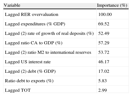
The final classification identified six variables with an overall importance greater than 45%: real exchange rate overvaluation (t − 1), expenditures as percentage of the GDP (t − 1), rate of growth of real total bank deposits (t − 2), ratio of current account to the GDP (t − 1), U.S. interest rates (t − 1) and the ratio of the monetary aggregate M2 to international reserves (t − 2). There were also four variables that had smaller importance: sovereign debt as percentage of GDP (t − 1), terms of trade (t − 1), real imports growth (t − 1) and the ratio of debt to exports (t − 1). It is worth noting that the variables with the highest importance in predicting crises were related to domestic policies rather than to exogenous shocks from abroad. The international interest rate with 59.6% of overall importance and the terms of trade with 3.6% came in the fifth and eighth place, respectively, in the ranking of overall importance of the variables, which seems very reasonable given that the Argentine economy exhibited a very low degree of openness to international trade for almost six decades, from the early 1930s to the late 1980s. In other words, “imported ingredients” that played into the Argentine crises were made mainly with domestic condiments.

The overall importance of variables, based on the contribution that predictors make to the construction of the tree, is presented in Table 3.

Table 3.

Overall importance of variables.

Variable	Importance (%)
Lagged RER overvaluation	100.00
Lagged expenditures (% GDP)	69.52
Lagged (2) rate of growth of real deposits (%)	52.49
Lagged ratio CA to GDP (%)	57.29
Lagged (2) ratio M2 to international reserves	53.72
Lagged US interest rate	46.17
Lagged (2) debt (% GDP)	17.02
Ratio debt to exports (%)	5.83
Lagged TOT	2.99

Notice that the 1929/1931 crisis known worldwide as the Great Depression had crisis years belonging to different splits. The crisis years 1929 and 1931 were included in the second mix while the crisis year 1930 was in the first mix.

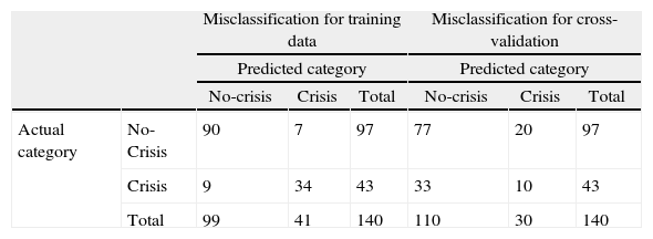
3.3

Misclassification

The resulting rate of misclassification for the entire group of observations was relatively low at 11%. Moreover, as soon as we analyzed each case separately, we found that there was only a small discrepancy between the CTA classification and the MTI identification. Table 4 shows the misclassification for the training dataset and the misclassification for the trees built for cross-validation. There were 16 misclassified crisis years for the training data and the 53 misclassified crisis years for cross-validation. From the training data, we observed that only 9 crises years out of 43 were predicted as non-crises: 1884, 1885, 1889, 1920, 1949, 1951, 1958, 1975 and 1990. Notice that we only failed to identify three crises: the deep episodes of 1884–1885 and 1958 that were signaled in 1882 and 1959, respectively, and the mild crisis of 1951, which was overlooked. For the rest of the crises with more than one crisis year, we correctly classified at least one crisis year. For example, our tree misclassified the crisis year 1889 but included the crisis year 1890, both belonging to the 1889–1890 crisis. Misclassified crises in the period 1940–1976 presumably were the consequence of a missing component of the MTI: the interest rate.

Table 4.

Misclassification for training data and cross-validation summary table.

		Misclassification for training data			Misclassification for cross-validation
		Predicted category			Predicted category
		No-crisis	Crisis	Total	No-crisis	Crisis	Total
Actual category	No-Crisis	90	7	97	77	20	97
	Crisis	9	34	43	33	10	43
	Total	99	41	140	110	30	140

There were also seven non-crises years out of the 97 that were predicted as crisis years: 1882, 1959, 1961, 1984, 1996, 1997 and 1999. As already mentioned, 1882 can be considered an early signal of the 1884–85 deep crisis and 1959 as a late signal of the 1958 deep crisis. Similarly, 1961 anticipated the deep crisis of 1962. Instead, the misclassification of 1984 can be attributed to the fact that it came between two crises: 1980–1983 and 1985. The misclassification of 1996, 1997 and 1999 may have been provoked by the mild turbulences related to the international crises of Southeast Asia and Russia.

3.4

Related empirical literature: a comparison

Most of the “ingredients” we found in our study were also present in Kaminsky's (2006) analysis for the period 1970–2002. She identified eight crises in Argentina that fell into three varieties, labeled “Financial Excesses,” “Sovereign Debt,” and “Current Account,” having the real exchange rate overvaluation as a common ingredient.¹² As in our paper, domestic economic fragilities were crucial to explaining crises, but different from us, she assigned no role at all to international interest rates as we did in the first mix, including the 1990/1991 crisis. In her classification, the crises of 1975, 1981 and 1982 corresponded to the financial excesses variety because they were preceded by acceleration in the growth rate of domestic credit and other monetary aggregates. On the other hand, Kaminsky assigned the crises of 1986, 1989 and 1990 to the sovereign-debt variety due to the presence of “unsustainable” foreign debt indicators such as high ratios of debt to exports and M2 to reserves. In our classification, these six crises were characterized by high public expenditures and current account deficits. Both results were closely related: During the 1980s, public expenditure, fiscal deficit, debt and monetary aggregates were highly correlated. Domestic disequilibria were initially financed with capital inflows from abroad but as the access to international and local credit markets were reduced, authorities resorted to money printing, which spurred inflation.¹³ Various attempts to anchor inflation by fixing the exchange rate resulted in a reserve drainage and a decline in the country's competitiveness.

Our “ingredients” were also similar to the determinants of Argentine crises obtained by Cerro and Meloni (2013). Using bivariate logit regressions, they concluded that expansions in public expenditures as well as augmentations in the debt to the GDP ratio, and diminishments in the rate of growth of bank deposits contributed to an increase in the probability of a crisis. Our results, reported in Table 3, show that Expenditure (as % of GDP) and the Rate of Growth Bank Deposits ranked 2nd and 3rd, respectively, as predictors of crises. Cerro and Meloni (2013) also noted that unfavorable external conditions, represented by the LIBOR rate in their paper, jointly with domestic imbalances, helped to explain very deep crises or crashes. Our classification tree shows that the U.S. interest rate, which was highly correlated with LIBOR in most of the period under study, was very important to forecasting Argentine crises. The main difference between both papers is that real exchange rate overvaluation was not significant at usual levels in the logit analysis while it was the top predictor in the classification tree. Nonetheless, one must bear in mind that the two papers differ in objectives and methods. The added value of this paper is the identification of mixes that contribute to each crisis year while Cerro and Meloni (2013) focused on the determinants of all crises from 1865 to 2002 with no involvement in particular crises.

4

Computing crises costs

The purpose of this section is to measure the most obvious cost of crises: output drops.¹⁴ We implemented a variant of the IMF's (1998) methodology to calculate the cumulative output loss relative to trend. Our computation involved three simple steps. Firstly, we computed the average rate of growth of the GDP for each of the five sub-periods considered for the MTI. Secondly, we compared the actual GDP growth in each crisis year with the GDP's average growth rate. Finally, the cost of output loss was estimated by adding the difference between the average GDP growth rate in a given sub-period and the actual GDP growth in the crisis year. For example, the cost of the 2000–2002 crisis was 23.97%. To obtain this result, we computed the difference between the average GDP growth rate for the sub-period 1991–2004, that is 2.62%; and the rate of growth of real GDP in each crisis year, that is −0.79% for 2000, −4.4% for 2001 and −10.89% for 2002. Hence, the crisis cost for 2000 was 2.62% + 0.79% = 3.41%. Similarly, for 2001 was 2.62% + 4.40% = 7.03% and for 2002 was 2.62% + 10.89% = 13.52%. Summing up, the cost for the three years was 23.97%.

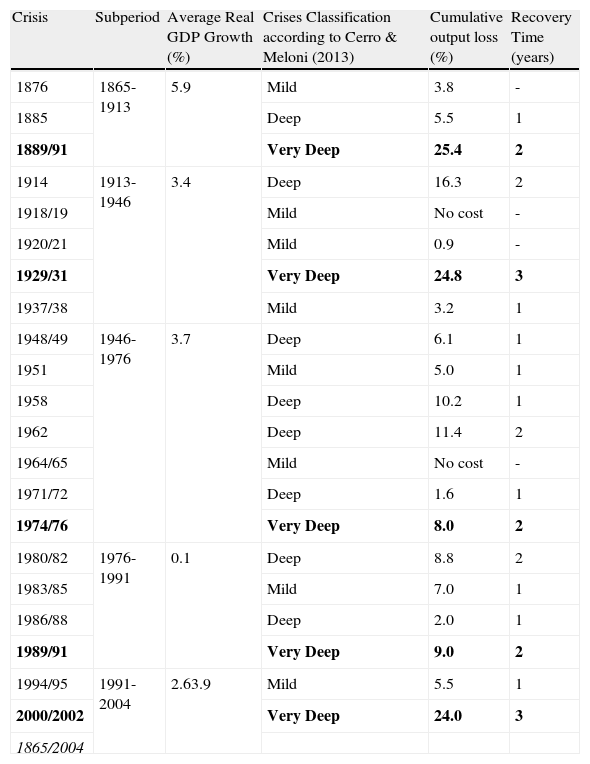
As a byproduct we also computed the recovery time from a crisis, that is, how long it took for the GDP growth to return to its average growth in the sub-period. Table 5 exhibits the results for the period 1865–2004.

Table 5.

Cumulative Output Loss and Recovery Time: 1865-2004.

Crisis	Subperiod	Average Real GDP Growth (%)	Crises Classification according to Cerro & Meloni (2013)	Cumulative output loss (%)	Recovery Time (years)
1876	1865-1913	5.9	Mild	3.8	-
1885			Deep	5.5	1
1889/91			Very Deep	25.4	2
1914	1913-1946	3.4	Deep	16.3	2
1918/19			Mild	No cost	-
1920/21			Mild	0.9	-
1929/31			Very Deep	24.8	3
1937/38			Mild	3.2	1
1948/49	1946-1976	3.7	Deep	6.1	1
1951			Mild	5.0	1
1958			Deep	10.2	1
1962			Deep	11.4	2
1964/65			Mild	No cost	-
1971/72			Deep	1.6	1
1974/76			Very Deep	8.0	2
1980/82	1976-1991	0.1	Deep	8.8	2
1983/85			Mild	7.0	1
1986/88			Deep	2.0	1
1989/91			Very Deep	9.0	2
1994/95	1991-2004	2.63.9	Mild	5.5	1
2000/2002			Very Deep	24.0	3
1865/2004

Source: Cerro and Meloni (2003, 2013) and own calculations.

The disparity of annual average GDP growth rates in different sub-periods prevented us from comparing crisis costs among sub-periods, so we will refer only to crisis costs within each sub-period.

The most important crisis in the sub-period 1865–1913 was the 1890–1991 crisis. The magnitude of the crash is explained by the default of sovereign debt and the banking crisis (most private and public banks declared bankruptcy). GDP fell 8.3% in 1890 and 5.4% in 1891. Given that Argentina grew at the outrageous rate of 5.9% between 1865 and 1913, the output loss was 25.4%. Fig. 5 illustrates the evolution of GDP and the crisis years in the 19th century.

Fig. 5.

Crises and GDP evolution: 1865–1899.

Source: Own calculations based on Ferreres (2005).

The first crisis of the 20th century, which occurred in 1914, was very expensive, too (16.3%). This crisis is associated with the beginning of World War I and the end of almost 14 years of convertibility under the gold standard regime. The high cost of this crisis is explained by the huge fall in GDP (10.4%) and the amazing average annual growth rate during the sub-period 1865–1914 (5.9%). The dearest crisis in the first half of the 20th century was The Great Depression. Cumulative output loss was enormous (almost 24%) and the recovery time was three years, from 1929 to 1931.

During the sub-period 1930–1975, there were eight crises with important output losses, but only the ones in 1958 and 1962 surpassed the 10% threshold. As the country's trend of the GDP growth diminished, and crises repeated with certain regularity, costs became relatively low. That is why crises classified as “very deep” by the MTI, like the 1974/76 and 1989/91, cost “only” 6.5% and 7% respectively. At the beginning of the 20th century, the country fell from high levels of a GDP growth trend, while at the end of the century, it fell from a very modest GDP growth trend. For example, the 1989/1991 crisis was the culmination of a decade characterized by continuous crises and consequent poor performance measured by output growth. Hence, recovering the GDP growth to the prevailing levels previous to the crash demanded a relatively small increase in output. Fig. 6, Panels A, B and C, shows the behavior of the GDP in the sub-periods 1900–1932, 1933–1976 and 1977–2004.

Fig. 6.

Evolution of GDP and Crises.

Panel (A) 1900–1932, Source: Own calculations based on Ferreres (2005). Panel (B) 1933–1976, Source: Own calculations based on Ferreres (2005). Panel (C) 1977–2004 Source: Own calculations based on Ferreres (2005).

4.1

The costs of each type of crisis

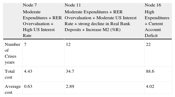
Which is the most expensive mix? We compared the costs involved in each of the three nodes of the CTA. Table 6 exhibits the cumulative output loss of each node. When episodes involved more than one crisis year belonging to different mixes, we computed the average cost.

Table 6.

Cumulative Output Loss Classified by Node. 1865-2004.

	Node 7	Node 11	Node 16
	Moderate Expenditures + RER Overvaluation + High US Interest Rate	Moderate Expenditures + RER Overvaluation + Moderate US Interest Rate + strong decline in Real Bank Deposits + Increase M2 (%R)	High Expenditures + Current Account Deficit
Number of Crises years	7	12	22
Total cost	4.43	34.7	88.6
Average cost	0.63	2.89	4.02

The most costly and frequent crises were the ones grouped in Node 16. We have 22 crisis years characterized by high public expenditure relative to GDP and current account deficits. The total cost was 88.6%, with an average cost of 4.02% per year of crisis. This result is in line with Kaminsky's (2006) conclusions. She found that, on average, the costs of crises with financial excesses were significantly higher than those of other crises, with crises of debt problems being a close second. Notice that most of the crisis years we reported in Node 16 were included in Kaminsky's financial excesses variety.

Crises in Node 7, characterized by moderate public expenditures relative to GDP, real exchange overvaluations, and high U.S. interest rates, were the less frequent and less costly. The total cost was 4.43%, with only 7 crisis years, and an average cost of 0.63%. Most of the crises involved in this node were mild crises.

The twelve crisis years classified in Node 11, featuring moderate public expenditures relative to GDP, real exchange overvaluations, moderate U.S. interest rates, but strong declines in real bank deposits and increased ratio of M2 to international reserves, had an average cost of 2.89%.

5

Concluding remarks

This paper constitutes one step in a broader scholarly agenda to understand crisis and to measure crisis costs. Identifying the “recipes” of the “explosive mixes” is crucial to generating an early warning system to prevent future events and to diminish their costs.

Different from previous studies that analyze the case of Argentina, like Cerro and Meloni (2013) that worked with bivariate logit regressions, we investigated the “recipes” of Argentine currency crises by means of the Classification Tree Analysis that delivers the determinants of each crisis and group them by common factors. Grouping crises allowed us to evaluate Argentina's crises costs in terms of output losses and recovery time. Our paper also differentiates from Kaminsky (2006) who pioneered the use of CTA to study crises, by focusing on Argentina and covering a longer period, from 1865 to 2004.

We obtained three “recipes.” The most costly and frequent mix had two “ingredients”: high public expenditures (% of GDP) and current account deficits (% of GDP). The probability of crisis when these two ingredients are present is 77%.

The less frequent and less costly mix was made with moderate public expenditures, real exchange rate overvaluations, and high international interest rates. The chance of having a currency crisis when these factors act together is 100%.

Finally, there was a mix that has an 83% probability of generating a crisis: moderate public expenditures, real exchange rate overvaluations, moderate international interest rates, a strong decline in bank deposits, and a high ratio of monetary aggregate M2 to international reserves. The costs and frequency of this five-ingredient formula are intermediate.

Funding

Received financial support research council of the Nacional university of tucumán (CIUNT).

Proyects of F403 and F408 and also the promotion agency national science and technology, PICT 2008, Project 0822.

Sources

Breiman, L., Friedman, J., Olshen, R. and Stone, C., 1984. Classification and Regression Trees. Wadsworth & Brooks, Belmont, CA.

Cumby, R. and van Wijnbergen, S., 1989. Financial policy and speculative runs with a crawling peg: Argentina 1979–1981. J. Int. Econ. 27, 111–127.

della Paolera, G., Irigoin, A. and Bozolli, C., 2003. Passing The Buck: Monetary and Fiscal Policies in Argentina: 1953–1999. In: della Paolera, G. and Taylor, A. (Eds.). A New Economic History of Argentina, Cambridge University Press, pp. 46–86.

della Paolera, G., 1988. How the Argentine Economy Performed During the International Gold Standard: A Reexamination. University of Chicago (Unpublished thesis).

Gerchunoff, P. and Llach, L., 2003. El Ciclo de la Ilusión y el Desencanto. Editorial Ariel, Buenos Aires.

Lewis, R., 2000. An introduction to Classification and Regression Tree Analysis (CART), paper presented at the Annual Meeting of the Society for Academic Emergency, San Francisco.

Reinhart, C. and Kaminsky, G., 1999. The twin crises: the causes of banking and balance-of-payment problems. Am. Econ. Rev. 89 (3), 473–500.

Acknowledgments

This paper is part of an agenda that Cerro and Meloni started some years ago with the contribution of Adrián Amado. We thank Adrián for his direct and indirect input into this paper. We build on Cerro and Meloni (2003) and Amado, Cerro and Meloni (2004). We are grateful to Víctor Elías and the participants of the XXIX Annual Meeting of the Argentinean Economic Association and LACEA 2004 for comments and suggestions to earlier versions of this paper. We also thank Santiago Ruíz Nicolini and Sergio Sansón for their research assistance. Naturally, all errors are ours. We gratefully acknowledge the support of the Consejo de Investigaciones de la Universidad Nacional de Tucumán (CIUNT) Grants F 403 and F 408 and PICT 2008, Project 0822. The views expressed herein are those of the authors.