


This paper studies the behavior of the smile in the Warsaw Stock Exchange (WSE) during the volatile summer of 2011.We investigate the volatility smile derived from liquid call and put options on the Polish WIG20 index which option series expired on September 2011. In this period, the polish index has dropped about 20% in two weeks time. By linear interpolation, implied volatilities for moneyness points needed were calculated, then we construct 355 smile curves for calls and puts options to study and make some kind of smile-types classification. We propose seventeen types-smiles which represent all possible cases of three points (three moneynesses) graphical patterns. This classification is made basing upon relationship higher/equal/lower values of implied volatility for each of three points. Furthermore, we distinguish the convexity of pattern. We can note that smiles, smirks and ups are convex in shape, while reversed ones and downs are concave functions.
Este artículo analiza el comportamiento de la sonrisa de la volatilidad en la Bolsa de Varsovia (WSE) durante el volátil verano de 2011, derivada de las opciones más líquidas sobre el índice polaco WIG20, cuyas series expiraron en septiembre de 2011. En ese período, el índice había caído aproximadamente un 20% en tan sólo dos semanas. Mediante interpolación lineal construimos 355 curvas de sonrisas para poder estudiar una posible clasificación o tipología de las mismas. Proponemos 17 tipos de sonrisas, las cuales representan todos los casos posibles de tres monetizaciones de patrones gráficos. Esta clasificación se basa en la relación valores superiores/iguales/inferiores de la volatilidad implícita para cada uno de los tres puntos. Además, se distingue la convexidad de cada una. Destacamos que las sonrisas completas, las sonrisas asimétricas y las inclinadas hacia arriba son de forma convexa, mientras que las invertidas y las inclinadas hacia abajo son funciones cóncavas.
Volatility measures how much prices move. The direction of the move, whether up or down, is irrelevant. The magnitude and the speed of the change are most important. In the futures and options markets, the implied volatility is often used, which refers how much the market anticipates price changes and is reflected on the prices of contracts. Implied volatility is used independently or together with historical volatility and other different methodologies (Stochastic volatility models, GARCH1 models, EWMA,2 etc.) to estimate the future volatility (see Covring & Low, 2003 and Wong & Tu, 2009, for instance). Whereas historical volatilities are “backward looking”, implied volatilities are “forward looking”. According to Duque and Teixeira Lopes (2003), the “Smile effect” is a result of an empirical observation of the options’ implied volatility, with the same expiration date, across different exercise prices. It typically describes a U-shape form showing high implied volatility patterns for in and out-of-the-money options (ITM & OTM) and low volatility figures for at-the-money options (ATM), that is, the implied volatility is relatively low for ATM options, but becomes progressively higher as an option moves either into the money or out of the money.
In this paper, we investigate the volatility smile derived from call and put options on the Polish WIG20 index, the nearest to expiring date, which are the most heavily traded and fluid index options in the Warsaw Stock Exchange. We also look into the procedures to obtain implied volatilities in order to compare different smiles and provide a pattern of them in the Polish market.
The paper is organized as follows. We start by reviewing the related literature as theoretical background. Next we describe the methodology in use and data. Finally, we present the empirical results and conclusions.
2Theoretical backgroundOver the years, it has become quite clear that the market does not price all options according to the Black–Scholes formula (Mayhew, 1995). The consensus opinion is that the model performs reasonably well for ATM options with one or two months to expiration and this experience has motivated the choice of such options for calculating implied volatility. For other options, however, the discrepancies between market and Black–Scholes prices are large and systematic. Because the Black–Scholes model holds reasonably well for some options and not for others, different options on the same underlying security must have different Black–Scholes implied volatilities. It is well known that the implied volatilities of options differ systematically across strike price and across time to expiration. The pattern of implied volatilities across times to expiration is known as the “term structure of implied volatilities”, and the pattern across strike prices is known as the “volatility skew” or the volatility smile. If we combine the skew with the term structure, we will obtain what is called “volatility surface”.
The earliest papers that found evidence for volatility smiles described how Black–Scholes pricing errors vary systematically with strike price or with time to expiration. Macbeth and Merville (1979), for example, reported that the Black–Scholes model undervalues ITM and overvalues OTM call options. Subsequent authors found the contrary result, that the Black–Scholes model undervalues OTM calls. These and other relevant results are summarized by Galai (1983).
The most systematic and complete study documenting volatility smiles is that of Rubinstein (1985), whose most robust result is that for OTM calls implied volatility is systematically higher for options with shorter times to expiration. His other results were statistically significant but changed across subperiods. Thus, systematic deviations from the Black–Scholes model appear to exist, but the pattern of deviations varies over the time. Culumovic and Welch (1994) found the same results using more recent data in a similar study.
Subsequent studies by Sheikh (1991) and by Heynen (1994) used Rubinstein's nonparametric tests to examine implied volatility patterns in index options. Sheikh found smile effects using transactions data for OEX call options from March 1983 to March 1987. Heynen examined the implied volatility of European Options Exchange (EOE) stock index options. Using Rubinstein's approach and transaction data from January 23 to October 31, 1989, he found systematic smile effects, including a U-shaped term structure of implied volatility.
Many other authors found evidence for volatility smiles and non-flat term structures of implied volatilities in various markets. Shastri and Tandon (1986), for example, used Geske and Johnson approach (1984) to price American options on futures and found volatility smile and term structure effects in the markets for options on S&P 500 futures and on Deutschemark futures. Xu and Taylor (1994) examined the term structure of volatility implied by options on four Philadelphia Stock Exchange currency options using data from 1985 to 1989. Heynen, Kemna, and Vorst (1994) examined the ability of various GARCH models to explain the observed term structure of implied volatilities. McKenzie, Gerace, and Subedar (2007) evaluated the probability of an exchange traded European call option being exercised on the ASX200 Options Index.
Related literature studies how the economic variables associated with the options market affect the volatility shape (Bollen & Whaley, 2004; Deuskar, Gupta, & Subrahmanyam, 2011; Dumas, Fleming, & Whaley, 1998; Ederington & Guan, 2002; Heynen et al., 1994; Hull & White, 1987; Jarrow, Li, & Zhao, 2007; Peña, Rubio, & Serna, 1999, 2001; Rompolis & Tzavalis, 2010).
Duque and Paxson (1994) found the smile effect for options traded on the London International Financial Futures and Options Exchange (LIFFE) during March 1991. Gemmill (1996) also found the same effect for options on the FTSE 100 during a 5-year period (from 1985 to 1990), although the smile showed different patterns for different days extracted from the sample. Dumas, Fleming, and Whaley (1998) also found empirical smile patterns for options on the S&P 500 stock index, but its shape seemed to be asymmetric and changing along time to maturity. Peña, Serna, and Rubio (1999) also found empirical smiles for stock index options written on the IBEX-35, for a time period between 1994 and 1996, detecting a day of the week effect for the smile. Low (2000) using the implied Market Volatility Index (VIX) of the Chicago Board Options Exchange (CBOE) found empirical evidence for the association between market conditions and volatility. However, his findings point to an asymmetric behavior for this relationship. Carverhill, Cheuk, and Dyrting (2002) showed evidence of the “smirk”, when studying deep away-from-the money index options. Lim, Martin, and Martin (2002) presented evidences for relatively symmetric imperfections (as it is regularly pointed out to the currency market) with a frown configuration for tranquil periods. Engström (2002) also found empirical evidence for the U-shaped smile for equity options written on Swedish stocks. Pan (2002) analysing stock index options quoted in the CBOE from 1989 to 1996 observed that jump models could accommodate a plausible assumption to justify a significant share of the smile. Wong and Tu (2009) studied the information content of option implied volatility and realized volatility under market imperfections in the context of GARCH modeling and volatility forecast of Taiwan stock market index ((TAIEX) returns. Other authors tried to extract superior information from the smile, as in Bates (1991), concluding that persistence on the smile pattern could imply that the market expected the 1987 crash.
Today it is common to justify the smile based on asymmetric and non-lognormal implied volatility distributions (see Hull, 2012). In order to match the empirical distributions several authors suggested models that accommodate jump, stochastic volatility or both, such as Gkamas and Paxson (1999), Das and Sundaram (1999), León and Rubio (2004) or Kuo (2011).
Some other authors impute the smile to the behavior of traders or to their risk aversion, such as Bookstaber (1991), Grossman and Zhou (1996), Gemmill (1996), Dumas, Fleming, and Whaley (1998), Gemmill and Kamiyama (1997) among others. Some others attribute the smile to transaction costs, like Clewlow and Xu (1992, 1993), Constantinides (1997) and Peña, Serna, and Rubio (1999). Finally, Geske and Roll (1984) claim that smiles are a result of errors in valuing American options on stocks paying dividends prior to maturity.
Duque and Teixeira Lopes (2003) used liquid equity options on 9 stocks traded on the LIFFE between August 1990 and December 1991 in order to confirm two different hypothesis for testing two different phenomena: the increase of the smile as maturity approaches, and the association between the smile and the volatility of the underlying stock.
Nowadays, most of the exchanges adopt different settlement practices for the options with low liquidity and thin trading. For example, the Japan Securities Clearing Corporation obtains the trading-volume-weighted average of the implied volatilities for all available equity index options to calculate the settlement price in a flat volatility structure (Chang, Ren, & Shi, 2009). In the Hong Kong options markets, the structure of implied volatility has significantly affected settlement prices. In order to decide the settlement prices of options in the Hang Seng Index (HIS), the Hong Kong Stock Exchange (HKEx) builds a smile implied volatility with three parameters provided by market makers. Chang et al. (2009) addressed the question of whether the structure of implied volatility set by market makers is consistent with the volatility pattern driven by the market transaction data.
In order to evaluate the performance of the implied volatility, Szu, Wang, and Yang (2011) investigate the characteristics of the settlement-price-determined and market-force-driven implied volatilities for the TAIEX options from January 2002 to December 2007. The empirical results reveal that a linear settlement practice generally induces a smile implied volatility pattern for the options expiring in the current and next month, while the market transaction data yield a smile volatility curve.
In conclusion, according to Duque and Teixeira Lopes (2003) we conclude that the literature is not unanimous in finding shapes as well as causes for smile effect and the models developed in order to cover this bias have only partially solved the problem.
3MethodologyThere are two important and independent features of the Black–Scholes Option Pricing Theory (1972, 1973): the risk-neutral valuation and the assumption that stock prices evolve lognormally with a constant volatility at any time and market level.
The only one parameter in the Black–Scholes pricing formulas that cannot be observed directly is the volatility of the underlying asset price (stock, index, foreign currency, etc.). The underlying asset price and the other parameters, including the strike price of the option, time to expiration, interest rate, and dividend yield of the underlying asset, are relatively easy to observe. Given that these values are known, the pricing formula relates the option price to the volatility of the underlying asset.
Historical stock price data may be used to estimate the volatility parameter, which then can be plugged into the option pricing formula to derive option values. As an alternative, one may observe the market price of the option then invert the option pricing formula to determine the volatility implied by the market price. When implied volatility increases, the market expects prices to move farther and/or faster. Consequently, option premiums will rise. Option writers will demand more money for the risk they are taking; option buyers are willing to pay more for the increased chance that the option will move ITM. When traders in the market believe prices are stabilizing, option premiums and implied volatility decrease (CME, 1988).
Implied volatilities can be used to monitor the market's opinion about the volatility of a particular stock. Traders often quote the implied volatility of an option rather than its price. This is convenient because implied volatility tends to be less variable than the option price. The implied volatility of an option does depend on its strike price and time to maturity. The implied volatilities of actively traded options are used by traders to estimate appropriate implied volatilities for other options (Hull, 2012).
Traditionally, implied volatility has been calculated using either the Black–Scholes formula or the Cox–Ross–Rubinstein binomial model (1979). Under the strict assumptions of the Black–Scholes model, implied volatility is interpreted as the market's estimate of the constant volatility parameter. If the underlying asset's volatility is allowed to vary deterministically over time, implied volatility is interpreted to be the market's assessment of the average volatility over the remaining life of the option. Option pricing formulas other than the Black–Scholes or Binomial also may be used to calculate implied volatilities. If the volatility of the underlying asset is itself a random process, as is assumed in stochastic volatility models, the market prices of options can still be used to estimate the parameters of the underlying asset process (Engle & Mustafa, 1992).
Option pricing formulas often cannot be inverted analytically, so implied volatility must be calculated numerically. In general, this calculation is accomplished by feeding the value-price difference:
where C(σ) is an option pricing formula, σ is the volatility parameter and CM is the observed market price of the option. Various algorithms can be used to find the value of σ that makes this expression equal to zero. Choosing among them involves a trade-off between robustness and speed of convergence. A simple approach that is very slow but reliable is to try a series of different values for σ and choose the one that comes closest to satisfying condition above. Sometimes known as the “shotgun method” (Mayhew, 1995), this approach is easy to implement but inefficient compared with other techniques such as the bisection method3 that for all practical purposes are just as robust. Faster convergence can be achieved if an analytic expression is known for the option's vega. Such is the case for the Black–Scholes formula, for a Newton–Raphson algorithm4 can usually achieve reasonably accurate estimates within two or three iterations. For a review of how apply both bisection and Newton–Raphson methods, see Kritzman (1991). Resorting to numerical procedures is not always necessary; for the special case of ATM options, Brenner and Subrahmanyam (1988) showed that the Black–Scholes formula can be inverted to derive a simple formula for implied volatility.
To calculate so-called “moneyness”, there are few ways to compound it. For instance, Duque and Teixeira Lopes (2003) define the moneyness degree of an option as:
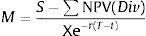
where S represents the underlying stock price, X represents the exercise price, r the risk free interest rate, T–t represents the time to maturity and NPV(Div) the net present value of the dividends paid on the stock until expiration. The moneyness degree of ATM options equals 1, for OTM call options it will be lower than 1 and for ITM options it will be greater than 1. They estimated the implied volatility of three specific moneyness degree, such as: M=1.06; M=1.00 and M=0.94. These are near ATM options and the exercise price interval [0.94; 1.06] is the range where option series are actively traded with higher open interest. Pan (2002) also selected a similar exercise price interval ([0.95; 1.05]).
In Kuo (2011), for Euribor futures and options traded in LIFFE, moneyness is defined as the futures price less the strike price for calls and the strike price less the futures price for puts with a moneyness degree such as: M≥0.1 (ITM); −0.1<M<0.1 (ATM) and M≤−0.1 (OTM). The skewed pattern indicates that OTM options are priced with greater volatility than those of ATM and ITM options and ITM volatilities are greater than ATM's, but are asymmetric around zero moneyness.
As moneyness could be calculated without time value and dividends, Eq. (2) could be written as:
where S represents the underlying stock price or index value and X the exercise price. It could also be used different levels of moneyness in percentage. For instance, a level of 5% gives an interval of [0.95;1.05], like Pan (2002); a level of 6% gives a interval of [0.94;1.06] like Duque and Teixeira Lopes (2003) or a level of 10% gives an interval of [0.90; 1.10]. These allow estimates implied volatilities under different groups of moneyness values the nearest or further from at-the-money level.
As the underlying stock price moves stochastically and the exercise prices are constant, daily observed moneyness of quoted options for the available exercise price change permanently. Therefore, it is impossible to extract daily implied volatilities with those exact moneyness degrees, directly from the available option premiums. In order to overcome this problem, volatility values for different points of moneyness for every day could be obtained (from implied volatilities for options with given strikes) by interpolation in different ways.
Interpolation is a method of constructing new data points within the range of a discrete set of known data points and provides a means of estimating the unknown function of implied volatility at intermediate points. There are many different interpolation methods such as the simplest Piecewise constant interpolation method or Nearest-neighbor interpolation, Linear interpolation (one of the simplest and widely-used methods), Polynomial interpolation (a generalization of linear interpolation) or Spline interpolation, which uses low-degree polynomials in each of the intervals, and chooses the polynomial pieces such that they fit smoothly together resulting a function called Spline. Other forms of interpolation can be constructed such as interpolation via Gaussian processes or by rational interpolation, trigonometric interpolation or the Whittaker-Shannon interpolation formula if the number of data points if infinite (see Marks II, 1991).
Duque and Teixeira Lopes (2003), like Clewlow and Xu (1993), used a B-spline curve in its cubic version to estimate the desired implied volatilities. B-spline curves (Gerald & Wheatley, 1994) are helpful instruments to draw non-linear functions from an irregular data set. In order to draw a piece of the desired function we need 4 data points. With these data points, the cubic version of B-spline enables us to draw a curve for the interval contained between the 2nd and the 3rd point.
In our paper, we applied linear extrapolation, where only two points to the left and right of moneyness calculated are needed, so with linear method it is possible to obtain more smiles, especially during high volatility periods, and allow us to estimate which type of smile it is, given by three moneyness points set.
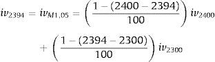
4DataThe WIG20 index is a capitalization-weighted stock market index of the twenty largest companies on the Warsaw Stock Exchange (WSE). Constituents of the WIG20 index are 20 companies with the highest position in the Ranking selected based on data following the last session of February, May, August and November. The Ranking is based on 12-month turnover values and free float market capitalization on the Ranking day. WIG20 is a price index and thus when it is calculated it accounts only for prices of underlying shares whereas dividend income is excluded.5 Options on Warsaw Stock Exchange have four strikes dates, these are third Friday of March, July, September and December. The calls are denominated C – March, F – June, I – September, L – December and puts O – March, R – June, U – September, X – December respectively. In the period under analysis (20 June–16 September 2011) strike prices were every 100 points of index WIG20. Polish option market is not very liquid unfortunately, options in-the-money, about 200 points and more from at-the money price are not intensively traded. At the beginning of period mentioned above, there were striking prices from 2100 up to 3300 and level of index WIG20 was about 2800 points (see Fig. 1). Between 1st and 11th September the index level went down from 2750 to 2111. The series with strike price 2000 were introduced in the market on 9th September, with strike prices of 1900 and 1800 on 11th September. It seems to be a little bit too late, but however, they were not much traded first days. Because on Warsaw Stock Exchange option market any reasonable liquidity is for option series nearest to the expiring date, we have taken into consideration September 2011-expiring series, it means OW20I (calls) and OW20U (puts) series. For others the trading is not high in the volume, and sometimes for hours on the bid/ask table there are only market-makers offers. In our paper we decided to use weighted average as a way to calculate values of volatility for chosen levels of moneyness. In this method only two points – one on the left side and one on the right side of moneyness value are needed. For example, to calculate ATM index value when actual WIG20 level is 2280 points, we take implied volatilities of 2300 and 2200 series iv2200 and iv2300, and:
The value of index (ind) for moneyness needed (for example 1.05) is calculated as follows:and for this value we calculate the weighted value of implied volatility in the same way as for at-the-money case above:The moneyness (M) is taken without time value, M=(actual index value)/(exercise price).

; daily differences between maximal and minimal value of WIG20 (right).")
The implied volatility values are taken from the Warsaw Stock Exchange official website following its method of achieving values.6
5Empirical resultsBelow, we propose some kind of classification of option volatility smiles which can be useful in our analysis. It concerns three points smile, which means that the center point is at-the-money level, while left and right equidistance under and above at-the-money. For example ±2% gives us levels of moneyness 0.98 and 1.02, so these three points will be 0.98; 1.00 and 1.02. In this paper we take under investigation three such groups of moneyness values: (0.98; 1.00; 1.02), (0.95; 1.00; 1.05) and (0.90; 1.00; 1.10).
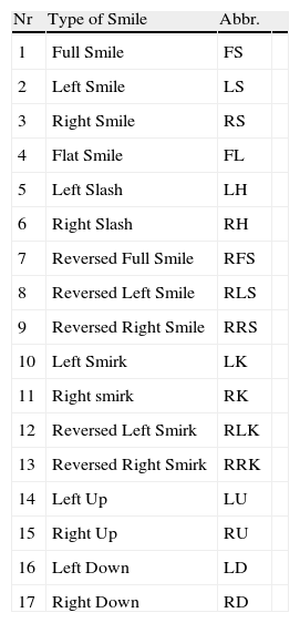
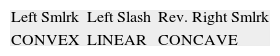
Option smiles classification, mentioned above, is presented in Table 1. These seventeen types which we propose here represent all possible cases of three points (three moneynesses) graphical patterns. Of course, Full Smile, Flat Smile, Reversed Full Smile, Left Down, Left Up, Right Down or Right Up are rather theoretical only. They could be taken into comparison also in the manner that the left and right points can differ in a little one from another to confirm this graph, for example, if the difference between left and right points does not exceed 10% of smile depth (left or right point value minus at-the-money point value). But in this paper we follow the precise, strict classification. This classification is made basing on relationship higher/equal/lower values of implied volatility for each of three points. Furthermore, we distinguish the convexity of pattern. For example, Left Smirk, Left Slash and Reversed Right Smirk have the same order of implied volatilities for consecutive points (the higher at the left and the lower at right hand side) but they have different convexity. Left Smirk is convex, Reversed Right Smirk is concave while Left Slash has linear dependence, so is between concave and convex (see Table 2).
Smile types classification.
| Nr | Type of Smile | Abbr. | |
| 1 | Full Smile | FS | |
| 2 | Left Smile | LS | |
| 3 | Right Smile | RS | |
| 4 | Flat Smile | FL | |
| 5 | Left Slash | LH | |
| 6 | Right Slash | RH | |
| 7 | Reversed Full Smile | RFS | |
| 8 | Reversed Left Smile | RLS | |
| 9 | Reversed Right Smile | RRS | |
| 10 | Left Smirk | LK | |
| 11 | Right smirk | RK | |
| 12 | Reversed Left Smirk | RLK | |
| 13 | Reversed Right Smirk | RRK | |
| 14 | Left Up | LU | |
| 15 | Right Up | RU | |
| 16 | Left Down | LD | |
| 17 | Right Down | RD |
Seven types have lower moneyness point with higher implied volatility, of course, also seven types – right moneyness points with higher volatility, and three types have the same level of left and right point (Full, Reverse Full and Flat Smiles). In three cases, ATM point has the lowest value (these are smiles), and three types have ATM point at the highest value (these are reversed smiles).
The Flat Smile is situation with no moneyness dependence, like in theoretical Black–Scholes option pricing model. In Smiles the at-the-money (the middle point) is always below or above (reversed smiles) other two points, while in Smirks, this at-the-money point has volatility between volatilities of two others. We can note that smiles, smirks and ups are convex in shape, while reversed ones and downs are concave functions.
In the previous Fig. 1 one can see, why the period chosen by us is so interesting. The value of main index of Warsaw Stock Exchange market WIG20 has fallen down by more than 500 points, which makes a drop of about 20% in two week time. The daily changes of this index had risen threefold–fourfold during period of drops. Fig. 2 presents illustrative volatility curves of put and call options in one-month intervals, it means one, two and three months to maturity day of these options. Characteristically, at the high-volatility day, the right tail of volatility curves situate higher, than before. Values of implied volatilities are then at least twice as those of months before. Fig. 3 introduces changes of implied volatility of ATM options versus time. Besides characteristic growing shape of time-dependence of implied volatility, we can observe here the jump of volatility between June and September.
 curves for call (left) and put (right) options with expiring day of 16.09.2011 versus moneyness.")
 curves for call (left) and put (right) options with expiring day of 16.09.2011 calculated for at-the-money points.")
For the highest volatility days, it means 9th and 10th September, in Fig. 4 “smile”-curves versus moneyness for call and put options are presented. The values of implied volatilities for moneyness below 1.00 (at 9th September) and 0.98 (at 9th 10th September) for calls were not possible to calculate because of nil-trading for options in these strike areas. It is noticeable that the values of implied volatility exceed here unusually rare value of 70%. Fig. 5 presents implied volatilities curves for the most volatile week for call and put options with expiring day of 16.09.2011 versus moneyness.
 curves for two days with the highest volatilities for call and put options with expiring day of 16.09.2011 versus moneyness.")
 curves for the most volatile week for call and put options with expiring day of 16.09.2011 versus moneyness.")
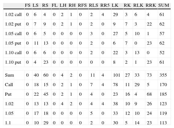
The smile type classification analysis is presented in Table 3. The most popular type, for both calls and puts, is Left Smirk (101 cases for 355 possible), rather than Reversed Right Smirk (73), Right Smile (60) and Left Smile (40). Never occurred seven theoretical types, it means Flat Smile, Reversed Full Smile, Left Up, Right Up, Left Down, Right Down and Full Smile. Left and Right Slash, as well as Reversed Right Smile have occurred only several times (no more than 4).
Number of smile types occurred on WSE for call and put options with expiring day of 16.09.2011 during the period 20.06.2011–16.09.2011 for three-point-smiles calculated with different moneyness (1.02 call means moneyness taken 0.98; 1; 1.02 for call options).
| FS | LS | RS | FL | LH | RH | RFS | RLS | RR5 | LK | RK | RLK | RRK | SUM | |
| 1.02 call | 0 | 6 | 4 | 0 | 2 | 1 | 0 | 2 | 4 | 29 | 3 | 6 | 4 | 61 |
| 1.02 put | 0 | 7 | 9 | 0 | 2 | 1 | 0 | 2 | 0 | 9 | 7 | 3 | 22 | 62 |
| 1.05 call | 0 | 6 | 5 | 0 | 0 | 0 | 0 | 3 | 0 | 27 | 5 | 10 | 1 | 57 |
| 1.05 put | 0 | 11 | 13 | 0 | 0 | 0 | 0 | 2 | 0 | 6 | 7 | 0 | 23 | 62 |
| 1.10 call | 0 | 6 | 6 | 0 | 0 | 0 | 0 | 2 | 0 | 22 | 3 | 13 | 0 | 52 |
| 1.10 put | 0 | 4 | 23 | 0 | 0 | 0 | 0 | 0 | 0 | 8 | 2 | 1 | 23 | 61 |
| Sum | 0 | 40 | 60 | 0 | 4 | 2 | 0 | 11 | 4 | 101 | 27 | 33 | 73 | 355 |
| Call | 0 | 18 | 15 | 0 | 2 | 1 | 0 | 7 | 4 | 78 | 11 | 29 | 5 | 170 |
| Put | 0 | 22 | 45 | 0 | 2 | 1 | 0 | 4 | 0 | 23 | 16 | 4 | 68 | 185 |
| 1.02 | 0 | 13 | 13 | 0 | 4 | 2 | 0 | 4 | 4 | 38 | 10 | 9 | 26 | 123 |
| 1.05 | 0 | 17 | 18 | 0 | 0 | 0 | 0 | 5 | 0 | 33 | 12 | 10 | 24 | 119 |
| 1.1 | 0 | 10 | 29 | 0 | 0 | 0 | 0 | 2 | 0 | 30 | 5 | 14 | 23 | 113 |
In Tables 3–5 smile types numbers 14–17 (Left Up, Right Up, Left Down, Right Down) are not presented in the columns because they did not occur at all.
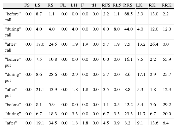
Frequency of smile types for three given periods, a period “before” – before jump of volatility: 20.06–2.08, a period “during” – during high volatility: 3.08–19.08, period “after” – after jump of volatility: 20.08–15.09.
| FS | LS | RS | FL | LH | F | tH | RFS | RL5 | RRS | LK | RK | RRK | |
| “before” call | 0.0 | 8.7 | 1.1 | 0.0 | 0.0 | 0.0 | 0.0 | 2.2 | 1.1 | 68.5 | 3.3 | 13.0 | 2.2 |
| “during” call | 0.0 | 4.0 | 4.0 | 0.0 | 4.0 | 0.0 | 0.0 | 8.0 | 8.0 | 44.0 | 4.0 | 12.0 | 12.0 |
| “after” call | 0.0 | 17.0 | 24.5 | 0.0 | 1.9 | 1.9 | 0.0 | 5.7 | 1.9 | 7.5 | 13.2 | 26.4 | 0.0 |
| “before” put | 0.0 | 7.5 | 10.8 | 0.0 | 0.0 | 0.0 | 0.0 | 0.0 | 0.0 | 16.1 | 7.5 | 2.2 | 55.9 |
| “during” put | 0.0 | 8.6 | 28.6 | 0.0 | 2.9 | 0.0 | 0.0 | 5.7 | 0.0 | 8.6 | 17.1 | 2.9 | 25.7 |
| “after” put | 0.0 | 21.1 | 43.9 | 0.0 | 1.8 | 1.8 | 0.0 | 3.5 | 0.0 | 8.8 | 5.3 | 1.8 | 12.3 |
| “before” | 0.0 | 8.1 | 5.9 | 0.0 | 0.0 | 0.0 | 0.0 | 1.1 | 0.5 | 42.2 | 5.4 | 7.6 | 29.2 |
| “during” | 0.0 | 6.7 | 18.3 | 0.0 | 3.3 | 0.0 | 0.0 | 6.7 | 3.3 | 23.3 | 11.7 | 6.7 | 20.0 |
| “after” | 0.0 | 19.1 | 34.5 | 0.0 | 1.8 | 1.8 | 0.0 | 4.5 | 0.9 | 8.2 | 9.1 | 13.6 | 6.4 |
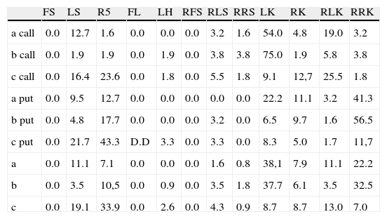
Frequency of smile types for three one-month periods, “a” period: 20.06–19.07, “b” period: 20.07–18.08, “c” period: 19.08–15.09.
| FS | LS | R5 | FL | LH | RFS | RLS | RRS | LK | RK | RLK | RRK | |
| a call | 0.0 | 12.7 | 1.6 | 0.0 | 0.0 | 0.0 | 3.2 | 1.6 | 54.0 | 4.8 | 19.0 | 3.2 |
| b call | 0.0 | 1.9 | 1.9 | 0.0 | 1.9 | 0.0 | 3.8 | 3.8 | 75.0 | 1.9 | 5.8 | 3.8 |
| c call | 0.0 | 16.4 | 23.6 | 0.0 | 1.8 | 0.0 | 5.5 | 1.8 | 9.1 | 12,7 | 25.5 | 1.8 |
| a put | 0.0 | 9.5 | 12.7 | 0.0 | 0.0 | 0.0 | 0.0 | 0.0 | 22.2 | 11.1 | 3.2 | 41.3 |
| b put | 0.0 | 4.8 | 17.7 | 0.0 | 0.0 | 0.0 | 3.2 | 0.0 | 6.5 | 9.7 | 1.6 | 56.5 |
| c put | 0.0 | 21.7 | 43.3 | D.D | 3.3 | 0.0 | 3.3 | 0.0 | 8.3 | 5.0 | 1.7 | 11,7 |
| a | 0.0 | 11.1 | 7.1 | 0.0 | 0.0 | 0.0 | 1.6 | 0.8 | 38,1 | 7.9 | 11.1 | 22.2 |
| b | 0.0 | 3.5 | 10,5 | 0.0 | 0.9 | 0.0 | 3.5 | 1.8 | 37.7 | 6.1 | 3.5 | 32.5 |
| c | 0.0 | 19.1 | 33.9 | 0.0 | 2.6 | 0.0 | 4.3 | 0.9 | 8.7 | 8.7 | 13.0 | 7.0 |
One can see from this table, that other patterns are typical for calls rather than puts. Typically calls are Left Smirk and Reversed Left Smirk, while for puts there are Reversed Right Smirk and Right Smile (this is more typical for bigger moneyness distance from ATM). These are presented below (Fig. 6):

With bigger distance from at-the-money (1.02→1.05→1.10) the number of Right Smiles increases, while left and Right Slashes as well as Reversed Right Smile appear only near-the-money (1.02 moneyness).
In Tables 4 and 5 analysis concerning time of appearance of specific type of smile is presented. First (Table 3), given period was divided into three as follows: before jump of volatility (20.06–2.08), during high volatility (3.08–19.08), after jump of volatility (20.08–15.09). Because of different period length the values in Table 4 are in percentage.
The “during” is a period related to high volatility time. Besides Right Smirk for puts, there are no other characteristic types of smile, which appears with considerably greater frequency. But other relationships could be observed here. Decreasing character of number of Left Smirks (for call options) from more than two-thirds to 7.5%, increasing of Right Smiles for both types of options and decreasing of Reversed Right Smirk for puts. So, in first period, Left Smirk is the most popular for calls and Reversed Right Smirk for puts. In second, Left Smirk is still the most popular for calls but with 24% less frequency, while for puts Right Smile and Reversed Right Smirk. The last period is a domination of Right Smile for puts and Reversed Left Smirk and Right Smile almost equally for calls. So, we can see here a changing character of smiles preferred.
Table 5 is similar, but here the summer period was divided into three, equal in length: “a” period: 20.06–19.07, “b” period: 20.07–18.08, “c” period: 19.08–15.09.
For call options in first two months the highest frequency is for Left Smirk, while in the last month before maturity Reversed Left Smirk, Right Smile and Left smile are the most common. For put options for first two months Right Reversed Smirk has the highest values, however for last month period it is Right Smirk which occurs the most frequent. Reversed Right Smile was never the case for put options, it occurred only for calls.
Comparing Tables 4 and 5, one can notice that, (1) for calls during volatility jump there were less Left Smirks than during b-period month (44% instead of 75%) and more RLK and RRK (12% instead of 5.8% and 3.8%); (2) for puts in the “during” high volatility period there were more Right Smiles (28.6% instead of 17.7%) but much less Reversed Right Smirks (25.7% instead of 56.5%).
6ConclusionsThis paper studies the behavior of the smile in the Warsaw Stock Exchange (WSE) during the volatile summer of 2011. In this period, the value of main index of Warsaw Stock Exchange market WIG20 has fallen down by more than 500 points, which makes a drop of about 20% in two weeks time. Polish option market is not very liquid, thus we investigate the volatility smile derived from call and put options on the Polish WIG20 index, the nearest to expiring date. We have taken into consideration September 2011-expiring series. The period analyzed (20 June–16 September 2011) was divided into three as follows: before jump of volatility (20/06–2/08), during high volatility (3/08–19/08), after jump of volatility (20/08–15/09). In order to estimate the implied volatility by linear interpolation, we have created a special program in Excel-VBA by ourselves and used weighted average as a way to calculate values of volatility for chosen levels of moneyness. 355 smile curves have been constructed for calls and puts options to study and make some kind of smile-types classification. We studied three triple points of moneyness every day of analysing period, and every triple was classified to one smile-type. Then, we compared all of them with typical shape pattern for calls, puts, different dates, etc. so we provide a pattern of them to the Polish market. In total, there are 170 smiles curves for call options and 185 for puts, corresponding to 2.7 call smiles and 2.9 put smiles on average per day. For those smiles, 52.1%, 16.9% and 31.0% correspond to first, second, and third sub-period, respectively.
The main result of the paper is to extend all theoretical graphics patterns to some kind of classification of option volatility smiles in WSE which can be useful for traders, investors, market makers, investment companies, etc. For instance, some smile types or characteristic changes in these types could be attached with changes of volatility or could anticipate changes in volatility (it should be important for traders on options volatility).
Seventeen types which we propose represent all possible cases of three points (three moneynesses) graphical patterns. This classification is made basing upon relationship higher/equal/lower values of implied volatility for each of three points. Furthermore, we distinguish the convexity of pattern. We can notice that smiles, smirks and ups are convex in shape, while reversed ones and downs are concave functions.
Analytical results reported that the most popular type, for both calls and puts, is Left Smirk (101 cases for 355 possible), rather than Reversed Right Smirk (73), Right Smile (60) and Left Smile (40). Seven theoretical types never occurred. Left and Right Slash, as well as Reversed Right Smile have occurred only several times (no more than 4).
Finally, the examination of volatility smile curves let us point out that decreasing character of number of Left Smirks (for call options) from more than two-thirds to 7.5%, increasing of Right Smiles for both types of options and decreasing of Reversed Right Smirk for puts. So, in first period, Left Smirk is the most popular for calls and Reversed Right Smirk for puts. In second, Left Smirk is still the most popular for calls but with 24% less frequency, while for puts Right Smile and Reversed Right Smirk. The last period is a domination of Right Smile for puts and Reversed Left Smirk and Right Smile almost equally for calls. In comparison with previous studies, smile patterns in the Warsaw Stock Exchange (WSE) differ from other option markets (LIFFE, CBOE, TWSE, OMX, etc.), which means each market smiles in some ways.
We believe that our research may modestly contribute to understand the volatility smile behavior in the Warsaw Stock Exchange. Future developments might compare how different the smile behave between Polish and Spanish options markets taking into consideration calls and puts options on IBEX-35.
Generalized auto regressive conditional heteroscedasticity.
Exponentially weighted moving average.
The bisection method is to bracket the root, then repeatedly cut the bracket in half to converge on the root.
The Newton–Raphson root-finding method speeds up convergence by taking advantage of information in the function's first derivate.
http://www.gpw.pl/indeksy_gieldowe_en?isin=PL9999999987&ph_tresc_glowna _start=show#portfolio –WIG20 – Main List Equity Index rules.


www.publicationethics.org.