Financial situation and political parties in local governments: Empirical evidence in the Spanish municipalities

Abstract

In contrast to several studies presented in the literature which analyze how different political elements affect specific aspects of financial management of public institutions, we have investigated from a comprehensive perspective how various political factors influence the financial situation of the municipalities. To do this, we use diverse multivariate techniques, the concept of financial condition and a large sample of Spanish municipalities. By isolating the electoral cycle and analyzing the essence of political factors, our main findings are that conservative and progressive parties do not present different behavior in relation to any of the financial dimensions. The territoriality of political parties influences the relationship between fund transfers received by the municipalities and certain expenses and investments. Furthermore, we did not detect that, in Spain, a partisan alignment exists between municipalities and the upper-level institutions.

Resumen

En contraste con los diversos estudios presentes en la literatura que analizan cómo los diferentes elementos políticos afectan a aspectos específicos de la gestión financiera de las instituciones públicas, hemos investigado desde una perspectiva integral cómo varios factores políticos influyen en la situación financiera de los municipios. Para ello hemos usado diversas técnicas multivariantes, el concepto de condición financiera y una amplia muestra de municipios españoles. Aislando el ciclo electoral y analizando la esencia de los factores políticos, nuestros principales hallazgos son que los partidos conservadores y progresistas no presentan distintas conductas en las diferentes dimensiones financieras, y que la territorialidad de los partidos políticos influye en la relación entre los fondos recibidos por transferencias y ciertos gastos e inversiones. Además, no hemos detectado que exista un alineamiento partidista entre los municipios españoles y las instituciones de nivel superior.

1

Introduction

Studies analysing the influence of political factors on specific aspects of financial management of public administrations, as deficit, expenditures, tax burden, revenues, public debt, and transfers at different territorial levels are, numerous (Benito & Bastida, 2010; Poterba, 1994; Rattsø & Tovmo, 2002; Roubini & Sachs, 1989; Solé-Ollé & Sorribas-Navarro, 2008; Veiga & Veiga, 2007).

Unlike these previous studies, García-Sánchez, Mordan, and Prado-Lorenzo (2012) analyzed the effect that political ideology and strength have on overall financial management of local governments through analysis of the financial condition concept in the largest Spanish municipalities. However, this study was limited because they directly assigned indicators to the financial dimensions, and performed individually the political variables on each of the indicators from a limited set. Furthermore, using various indicators which may reflect the same behavior tends to distort the analysis because this promotes the assessment of aspects in a duplicate manner (Cabaleiro, Buch, & Vaamonde, 2012).

Different from the rest of the studies presented in the literature, our paper is based on a more comprehensive vision that eliminates the analysis of redundant financial aspects and it intends to explain how different political factors such as ideology, political weakness of governments, and alignment between political hierarchical institutions (which have not presented conclusive results in previous works), or territoriality of political parties (which have not been empirically verified) may be influencing the overall financial health of local governments.

2

Literature review: background and hypotheses

2.1

The financial health of local governments

Various terms that correspond to different methodological approaches were used in the literature to analyze the same reality, the financial health (Berne, 1992; Clark, 1994; Carmeli, 2003; Kloha, Weissert, & Kleine, 2005; Wang, Dennis, & Tu, 2007), and the financial condition is one of the terms most widely used (Cabaleiro et al., 2012; Rivenbark & Roenigk, 2011; Sohl, Peddle, Thurmaier, Wood, & Kuhn, 2009; Wang et al., 2007). In this sense, Honadle, Costa, and Cigler (2004) noted that financial condition of local institutions is a term closely linked to the concept of fiscal health and Wang et al. (2007) pointed out that this concept represents the ability of an organization to meet its financial obligations on time.

As financial condition is a concept that is not directly observable, literature has focused on assessing the different aspects or dimensions that compose it (Clark, 1977; Groves, Godsey, & Shulman, 1981; Hendrick, 2004; Mercer & Gilbert, 1996). Groves et al. (1981) note that financial condition is composed of cash solvency (government's capacity to generate enough cash or liquidity to pay its bills), budgetary solvency (the city's ability to generate sufficient revenues over its normal budgetary period to meet its expenditure obligations and not incur deficits), long-run solvency (the long-run ability of a government to pay all the costs of doing business, including expenditure obligations that normally appear in each annual budget, as well as those that show up only in the years in which they must be paid), and service-level solvency (it refers to whether a government can provide the level and quality of services required for the general health and welfare of a community), and this approach was assumed by the International City/County Management Association [ICMA] (2003) for its extensive application in local governments in USA.

Another significant contribution for the local level is made by the Canadian Institute of Chartered Accountants [CICA] (1997, 2009) which assesses the concept through the dimensions of sustainability (degree to which a government can maintain its existing financial obligations without increasing the relative debt or tax burden on the economy within which it operates), flexibility (degree to which a government can change its debt or tax burden on the economy within which it operates to meet its existing financial obligations), and vulnerability (degree to which a government is dependent on sources of funding outside its control or influence or is exposed to risks that could impair its ability to meet its existing financial obligations).

To assess the financial condition, numerous indicators have been used. It should be noted that there has not been a common view in their selection, use, and application (CICA, 1997, 2009; Clark, 1977, 1994; Groves et al., 1981; Hendrick, 2004; ICMA, 2003).

On the contrary, the financial condition of governments and socioeconomic variables are interrelated aspects (Carmeli & Cohen, 2001; Honadle et al., 2004). The characteristics of a socioeconomic environment are diverse and varied in nature, that is, the economic sectors, nature of the territory, population structure and population movements, and economic policies developed by state public institutions (Honadle, 2003). In addition, the ICMA (2003) includes among the “environmental factors” the variables of population size, density, the level of unemployment, and business activity. Wang et al. (2007) analyzed the relationship between the financial condition and population (population size and growth rate) and economic factors (personal income per capita, gross state product per capita, and percentage change in personal income), and concluded that these variables can be used to predict the financial condition with a certain level of accuracy.

2.2

The political factors on the financial health of local governments

The ICMA (2003) considers that issues of a political nature must also be taken into account among the various factors to consider in the analysis of the financial management of public institutions. Except the limited study of García-Sánchez et al. (2012), there have been no empirical studies evaluating the relationship between the global financial situation of public institutions and political factors, although diverse political factors have been used to predict specific aspects of financial management (Alesina & Perotti, 1995; Alesina & Tabellini, 1990; Ashworth, Geys, & Heyndels, 2005; Benito & Bastida, 2010; Curto-Grau, Solé-Ollé, & Sorribas-Navarro, 2012; Solé-Ollé & Sorribas-Navarro, 2008).

A first political issue that we could not ignore is “The political cycle theory” or “Political opportunism”, which assumes that the primary interest of a politician or party is being re-elected and there are no ideological motives. Franzese (2002) notes that this theory is focused on the impact of the timing of elections, and this causes changes in some financial variables (debt, deficit, expenses, and transfers).

The “partisan theory” attributes central importance to the ideological differences between groups within a society and the parties that represent these groups (Persson & Svensson, 1989; Tuffe, 1978). In this line, unlike the conservative parties, progressives tend to increase public spending, showing greater laxity in public financial management (Tuffe, 1978). However, this theory has not been confirmed empirically in some studies at municipal level as in those made by Bosch and Suarez-Pandiello (1995) and Benito and Bastida (2010).

Some papers have examined the effect of political decentralization on the organization or cohesion of political parties (Desposato, 2004; Wildavsky, 1967). Territorial (local and regional) parties are thought to exist because these geographical areas have unique interests and concerns that cannot be or are not being addressed adequately by existing parties to other level (Brancati, 2008; Hearl, Budge, & Pearson, 1996).

Following the line of study based on “weak government” or “fragmented governments”, Roubini and Sachs (1989) initiated a line of empirical work studying the influence of fragmentation of governments on the finance of public institutions. At the municipal level, the works that researched any aspect of public finances have been few and they have also presented different results (Ashworth et al., 2005; Borge, 2005; Bruce, Carrol, Deskins, & Rork, 2007; Geys, 2007; Goeminne, Geys, & Smolders, 2008; Rattsø & Tovmo, 2002).

Another political factor is based on the “hypothesis of the partisan alignment”. In this context, the research carried out was articulated from different perspectives: “clientelism” (Diaz-Cayeros, Magaloni, & Weingast, 2006; Scheiner, 2005), “perverse accountability” (Stokes, 2005), and the “model of pork barrel” (Brollo & Nannicini, 2010; Solé-Ollé & Sorribas-Navarro, 2008). If there is a partisan alignment between the municipal government and the upper-level government, these entities receive larger fund transfers (Brollo & Nannicini, 2010; Diaz-Cayeros et al., 2006; Solé-Ollé & Sorribas-Navarro, 2008). The effect of a partisan alignment between regional and local governments has been considered in Spain by Solé-Ollé and Sorribas-Navarro (2008) and by Curto-Grau et al. (2012).

2.3

Hypotheses

According to the previous arguments, the aim of our study is concretized on the following hypotheses:Hypothesis 1

The ideology of the municipal government affects the dimensions of financial condition of the Spanish municipalities.

Hypothesis 2

The territoriality of political parties of the municipal government affects the dimensions of financial condition of the Spanish municipalities.

Hypothesis 3

The municipal government's weakness affects the dimensions of financial condition of the Spanish municipalities.

Hypothesis 4

The partisan alignment of the municipal government affects the dimensions of financial condition of the Spanish municipalities.

3

The financial health and political parties in Spanish local governments

3.1

Data

The very short data series available having adequate detailed financial information and the necessity to isolate the impact of political cycle on the global financial situation of the municipalities have forced us to use a transversal analysis, and then we chose the year 2009 because of its intermediate position in the electoral cycle of 2007–2011. The financial data for our study were collected from the databases of the “Settlement of the Local Budgets for 2009” and the “Municipal Debt Volume for 2009” (Ministry of Finances and Public Administrations). The data on socioeconomic indicators for 2009 were extracted from the “Municipal Database” of La Caixa and “Inebase” (National Statistics Institute). The information on the political variables was extracted from the “Database of Electoral Results” of the Ministry of Interior and the “Database of Mayors of Legislature 2007–2011” (Ministry of Finances and Public Administrations).

The work is focused on municipalities with more than 20,000 inhabitants and they represent 70% of the population in Spain. After cross-checking all the databases and eliminating municipalities with incomplete and missing data, Madrid and Barcelona because they have a special financial legislation, and Ceuta and Melilla for their different administrative systems, the sample has 387 of 399 municipalities with this population level.

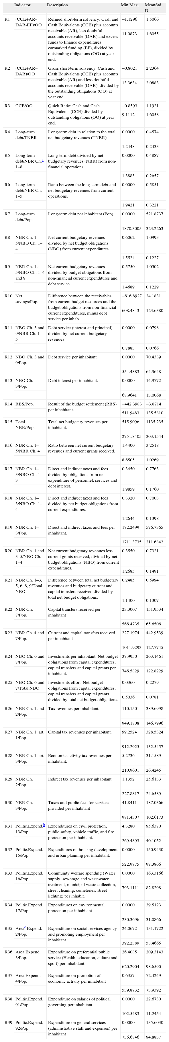
3.2

Methodology

The complexity of municipal finances analysis “requires that a mosaic of indicators be employed to account for the multitude of internal and external financial factors that comprise any given community's financial profile” (Sohl et al., 2009). In previous studies, the financial dimensions are measured through the assignment of indicators by the authors, with any exception (Clark, 1977; Mercer & Gilbert, 1996). However, an inconsistent use of indicators diminishes the reliability of a study (Sohl et al., 2009). For this reason, we used a wide set of financial ratios covering the numerous financial aspects or dimensions included in the approaches developed by ICMA (2003) and CICA (1997, 2009) because they are the more institutional relevant frameworks (see Table 1).

Table 1.

Financial indicators.

	Indicator	Description	Min.Max.	MeanStd. D
R1	(CCE+AR-DAR-EF)/OO	Refined short-term solvency: Cash and Cash Equivalents (CCE) plus accounts receivable (AR), less doubtful accounts receivable (DAR) and excess funds to finance expenditures earmarked funding (EF), divided by outstanding obligations (OO) at year end.	−1.1296	1.5066
			11.0873	1.6055
R2	(CCE+AR–DAR)/OO	Gross short-term solvency: Cash and Cash Equivalents (CCE) plus accounts receivable (AR) and less doubtful accounts receivable (DAR), divided by the outstanding obligations (OO) at year end.	−0.8021	2.2364
			13.3634	2.0883
R3	CCE/OO	Quick Ratio: Cash and Cash Equivalents (CCE) divided by outstanding obligations (OO) at year end.	−0.8593	1.1921
			9.1112	1.6058
R4	Long-term debt/TNBR	Long-term debt in relation to the total net budgetary revenues (TNBR)	0.0000	0.4574
			1.2448	0.2433
R5	Long-term debt/NBR Ch.^a 1–8	Long-term debt divided by net budgetary revenues (NBR) from non-financial operations.	0.0000	0.4887
			1.3883	0.2657
R6	Long-term debt/NBR Ch. 1–5	Ratio between the long-term debt and net budgetary revenues from current operations.	0.0000	0.5851
			1.9421	0.3221
R7	Long-term debt/Pop.	Long-term debt per inhabitant (Pop)	0.0000	521.8737
			1870.3005	323.2263
R8	NBR Ch. 1–5/NBO Ch. 1–4	Net current budgetary revenues divided by net budget obligations (NBO) from current expenditures	0.6062	1.0993
			1.5524	0.1227
R9	NBR Ch. 1 a 5/NBO Ch. 1–4 and 9	Net current budgetary revenues divided by budget obligations from non-financial current expenditures and debt service.	0.5750	1.0502
			1.4689	0.1229
R10	Net savings/Pop.	Difference between the receivables from current budget resources and the budget obligations from non-financial current expenditures, minus debt service per inhab.	−616.8927	24.1831
			608.4843	123.6380
R11	NBO Ch. 3 and 9/NBR Ch. 1–5	Debt service (interest and principal) divided by net current budgetary revenues	0.0000	0.0798
			0.7883	0.0766
R12	NBO Ch. 3 and 9/Pop.	Debt service per inhabitant.	0.0000	70.4389
			554.4883	64.9648
R13	NBO Ch. 3/Pop.	Debt interest per inhabitant.	0.0000	14.9772
			68.9641	13.0068
R14	RBS/Pop.	Result of the budget settlement (RBS) per inhabitant.	−442.3983	−3.8714
			511.9483	135.5810
R15	Total NBR/Pop.	Total net budgetary revenues per inhabitant.	515.9096	1135.235
			2751.8405	303.1544
R16	NBR Ch. 1–5/NBR Ch. 4	Ratio between net current budgetary revenues and current grants received.	1.4400	3.2518
			8.6505	1.0269
R17	NBR Ch. 1–3/NBO Ch. 1–3	Direct and indirect taxes and fees divided by obligations from net expenditure of personnel, services and debt interest.	0.3450	0.7763
			1.9859	0.1760
R18	NBR Ch. 1–3/NBO Ch. 1–4	Direct and indirect taxes and fees divided by net budget obligations from current expenditures.	0.3320	0.7003
			1.2644	0.1398
R19	NBR Ch. 1–3/Pop.	Direct and indirect taxes and fees per inhabitant.	172.2499	576.7365
			1711.3735	211.6842
R20	NBR Ch. 1 and 3–5/NBO Ch. 1–4	Net current budgetary revenues less current grants received, divided by net budget obligations (NBO) from current expenditures.	0.3550	0.7321
			1.2685	0.1491
R21	NBR Ch. 1–3, 5, 6, 8, 9/Total NBO	Difference between total net budgetary revenues and budgetary current and capital transfers received divided by total net budget obligations.	0.2485	0.5994
			1.1400	0.1307
R22	NBR Ch. 7/Pop.	Capital transfers received per inhabitant	23.3007	151.9534
			566.4735	65.6506
R23	NBR Ch. 4 and 7/Pop.	Current and capital transfers received per inhabitant	227.1974	442.9539
			1011.9293	127.7745
R24	NBO Ch. 6 and 7/Pop.	Investments per inhabitant: Net budget obligations from capital expenditures, capital transfers and capital grants per inhabitant.	37.9950	263.1461
			746.5829	122.8229
R25	NBO Ch. 6 and 7/Total NBO	Investments effort: Net budget obligations from capital expenditures, capital transfers and capital grants divided by total net budget obligations.	0.0360	0.2279
			0.5036	0.0781
R26	NBR Ch. 1 and 2/Pop.	Tax revenues per inhabitant.	110.1501	389.6998
			949.1808	146.7996
R27	NBR Ch. 1, art. 1/Pop.	Capital tax revenues per inhabitant.	99.2524	328.5324
			912.2925	132.5457
R28	NBR Ch. 1, art. 3/Pop.	Economic activity tax revenues per inhabitant.	5.2736	31.1589
			210.9601	26.4245
R29	NBR Ch. 2/Pop.	Indirect tax revenues per inhabitant.	1.1352	25.6133
			227.8817	24.6589
R30	NBR Ch. 3/Pop.	Taxes and public fees for services provided per inhabitant	41.8411	187.0366
			981.4307	102.6173
R31	Politic.Expend.^b 13/Pop.	Expenditures on civil protection, public safety, vehicle traffic, and fire protection per inhabitant.	4.3280	95.6370
			269.4893	40.1052
R32	Politic.Expend. 15/Pop.	Expenditures on housing development and urban planning per inhabitant.	0.0000	150.9430
			522.9775	97.3866
R33	Politic.Expend. 16/Pop.	Community welfare spending (Water supply, sewerage and wastewater treatment, municipal waste collection, street cleaning, cemeteries, street lighting) per inhabit.	0.0000	163.3166
			793.1111	82.8298
R34	Politic.Expend. 17/Pop.	Expenditures on environmental protection per inhabitant	0.0000	39.5123
			230.3696	31.0866
R35	Area^c Expend. 2/Pop.	Expenditure on social services agency and promoting employment per inhabitant.	24.0672	131.1722
			392.2389	58.4665
R36	Area Expend. 3/Pop.	Expenditure on preferential public service (Health, education, culture and sport) per inhabitant	26.4085	209.3143
			620.2904	98.6590
R37	Area Expend. 4/Pop.	Expenditure on promotion of economic activity per inhabitant	0.6357	72.4249
			539.8732	73.9392
R38	Politic.Expend. 91/Pop.	Expenditure on salaries of political governing per inhabitant	0.0000	22.6730
			102.5483	11.2454
R39	Politic.Expend. 92/Pop.	Expenditure on general services (administrative staff and expenses) per inhabitant	0.0000	135.6030
			736.6846	94.8837

Valid N (listwise) 387.

a

Chapter of the economic classification of the budgets in Spain.

b

Policy of expenditure on the Planning Programming Budgeting System in Spain.

c

Area of expenditure on the Planning Programming Budgeting System in Spain.

As each indicator may reflect aspects of more than one dimension (Cabaleiro et al., 2012), we will try to associate sets of indicators with similar variability to the dimensions conceptually defined by CICA and ICMA, using a multivariate statistical technique that attempts to overcome the limitations of previous works. In this sense, to assign univocally the ratios to the different financial aspects, we applied a sequential, agglomerative and non-overlapping method (hierarchical clustering with Ward method) based on the minimization of the variance of the dissimilarity measure of the squared Euclidean distance.

On each of the clusters of variables obtained, we applied factor analysis. The purpose is to find in each cluster a small number of uncorrelated aspects that explain the behavior of all the variables of the group with minimum loss of information. Consequently, the financial dimensions or sub-dimensions obtained by regression (dependent variables) are integrated by the groups of indicators that have similar variability, that is, similar behavior (Cabaleiro et al., 2012; Clark, 1977; Mercer & Gilbert, 1996). Each of these blocks/groups was identified in coherence with its information and by taking into account the financial dimensions or sub-dimensions from the ICMA and CICA frameworks.

To analyze how the political variables (ideology, territoriality of political parties, government weakness, and partisan alignment) (Table 2) might affect the dimensions that make up the financial condition of municipalities, we test if mean values are different. To do this, we performed an analysis of variance–covariance.

Table 2.

Political variables.

Political variable	Description	Freq	Relative freq (%)
(PV1) Ideology	Progressive (1)	204	52.7
	Conservative (2)	151	39.0
	Not defined (3)	32	8.3
(PV2) Territoriality of political parties	National (1)	321	82.9
	Regional (2)	46	11.9
	Local (3)	20	5.2
(PV3) Government weakness	Government party with absolute majority (1)	190	49.1
	Government party without absolute majority (0)	197	50.9
(PV4) Partisan alignment
(PV4_1) Provincial	The same political party that governs the municipality also governs the province (1)	235	60.7
	The political party that governs the municipality does not govern the province (0)	152	39.3
(PV4_2) Regional	The same political party that governs the municipality also governs the Autonomous Community (1)	213	55.0
	The political party that governs the municipality does not govern the Autonomous Community (0)	174	45.0

Valid N (listwise) 387.

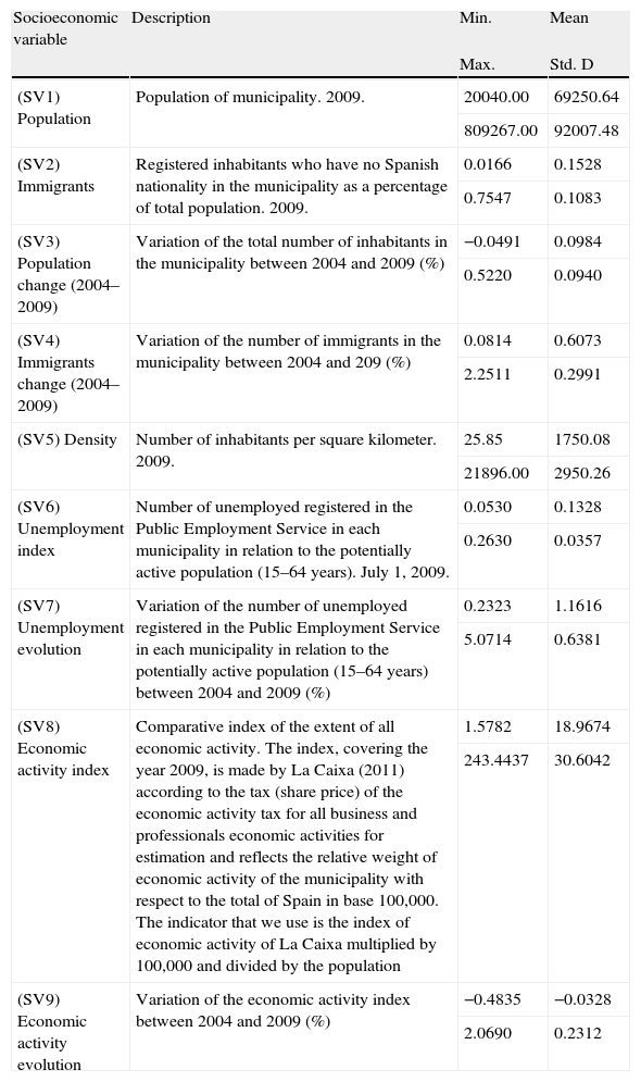
As noted above, socioeconomic factors are configured as elements of contrasted influence. For this reason, we must control the effect of demographic and economic environment variables (Table 3) on the financial condition of the municipalities.

Table 3.

Socieconomic variables.

Socioeconomic variable	Description	Min.	Mean
		Max.	Std. D
(SV1) Population	Population of municipality. 2009.	20040.00	69250.64
		809267.00	92007.48
(SV2) Immigrants	Registered inhabitants who have no Spanish nationality in the municipality as a percentage of total population. 2009.	0.0166	0.1528
		0.7547	0.1083
(SV3) Population change (2004–2009)	Variation of the total number of inhabitants in the municipality between 2004 and 2009 (%)	−0.0491	0.0984
		0.5220	0.0940
(SV4) Immigrants change (2004–2009)	Variation of the number of immigrants in the municipality between 2004 and 209 (%)	0.0814	0.6073
		2.2511	0.2991
(SV5) Density	Number of inhabitants per square kilometer. 2009.	25.85	1750.08
		21896.00	2950.26
(SV6) Unemployment index	Number of unemployed registered in the Public Employment Service in each municipality in relation to the potentially active population (15–64 years). July 1, 2009.	0.0530	0.1328
		0.2630	0.0357
(SV7) Unemployment evolution	Variation of the number of unemployed registered in the Public Employment Service in each municipality in relation to the potentially active population (15–64 years) between 2004 and 2009 (%)	0.2323	1.1616
		5.0714	0.6381
(SV8) Economic activity index	Comparative index of the extent of all economic activity. The index, covering the year 2009, is made by La Caixa (2011) according to the tax (share price) of the economic activity tax for all business and professionals economic activities for estimation and reflects the relative weight of economic activity of the municipality with respect to the total of Spain in base 100,000. The indicator that we use is the index of economic activity of La Caixa multiplied by 100,000 and divided by the population	1.5782	18.9674
		243.4437	30.6042
(SV9) Economic activity evolution	Variation of the economic activity index between 2004 and 2009 (%)	−0.4835	−0.0328
		2.0690	0.2312

Valid N (listwise) 387.

3.3

Analysis of results

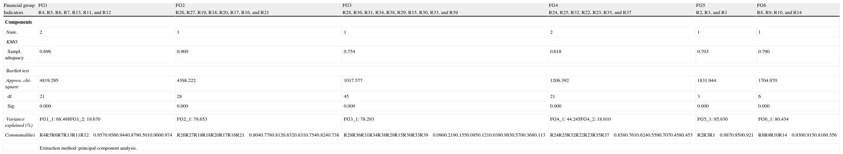
Following the methodological process described, after typifying all the financial variables (I1 to I39), we performed a cluster analysis of the variables. Fig. 1 shows the dendrogram where six groups of financial ratios (FG1 to FG6) can be clearly identified (see the cut line for rescaled distance = 10).

Fig. 1.

Clustering process of financial variables.

Following the methodology described, the technique of factor analysis was applied within each one of these groups and has led us to identify the following dependent variables, that is, financial groups (FG) (Table 4):

• -

  FG1 (R4, R5, R6, R7, R13, R11, and R12): They are basically indicators related to the dimension of long-term solvency. This group has two distinct behaviors or dimensions (factors). The first aspect gives more importance to the indicators related to the volume of debt of the entity (R4, R5, R6, R7, R13) (FG1_1). The second behavior gives more importance to the indicators R1 and R12 and an opposite direction to the other. This refers to the speed with which the entity is to amortize its debt (FG1_2).

• -

  FG2 (R26, R27, R19, R18, R20, R17, R16, and R21) represents a homogeneous group of indicators essentially concerned with budgetary solvency derived from the entity's ability to generate its own income (FG2_1).

• -

  FG3 (R28, R36, R31, R34, R38, R29, R15, R30, R33, and R39) basically consists of a set of service ratios and income tax ratios related to economic activity in the municipal environment with similar variability to all local government revenue. This seems to reflect a level of solvency of services of each entity, which is linked to the activity of local economic environment (FG3_1).

• -

  FG4 (R24, R25, R32, R22, R23, R35, and R37). This group is composed of indicators of transfers, investments, and certain spending policies. This seems to reflect a degree of financial dependence on other institutions to provide certain services and investment. The factor analysis shows the existence of two distinct behaviors or dimensions. The first shows a similar behavior between transfers received and transfers made, the real investments, and housing and urban policies and to a lesser extent, the spending policies of social protection and economic policies (FG4_1). The second component reflects a different behavior of the policies of social protection expenditure and economic policies in relation to investments and transfers made (FG4_2); that is, it displays the extent to which the local entity opts for performing one or other expenses.

• -

  FG5 (R2, R3, and R1): The group is only composed of indicators of short-term solvency or cash solvency (FG5_1).

• -

  FG6 (R8, R9, R10, and R14): The group is only composed of indicators of current and overall balanced budget. This represents general budgetary solvency (FG6_1).

Table 4.

Process of factor analysis.

Financial group	FG1		FG2		FG3		FG4		FG5		FG6
Indicators	R4, R5, R6, R7, R13, R11, and R12		R26, R27, R19, R18, R20, R17, R16, and R21		R28, R36, R31, R34, R38, R29, R15, R30, R33, and R39		R24, R25, R32, R22, R23, R35, and R37		R2, R3, and R1		R8, R9, R10, and R14
Components
Num.	2		1		1		2		1		1
KMO
Sampl. adequacy	0.696		0.900		0.754		0.618		0.703		0.790
Bartlett test
Approx. chi-square	4819.295		4398.222		1017.577		1206.392		1831.944		1704.970
df	21		28		45		21		3		6
Sig.	0.000		0.000		0.000		0.000		0.000		0.000
Variance explained (%)	FG1_1: 68.498FG1_2: 19.670		FG2_1: 79.653		FG3_1: 78.293		FG4_1: 44.245FG4_2: 18.910		FG5_1: 95.930		FG6_1: 80.434
Communalities	R4R5R6R7R13R11R12	0.9570.9560.9440.8790.5010.9600.974	R26R27R19R18R20R17R16R21	0.8040.7780.8120.8320.8310.7540.8240.738	R28R36R31R34R38R29R15R30R33R39	0.0900.2190.1550.0950.1210.0380.9930.5700.3680.113	R24R25R32R22R23R35R37	0.8580.7610.6240.5590.7070.4580.453	R2R3R1	0.9870.9500.921	R8R9R10R14	0.9300.9150.8160.556
	Extraction method: principal component analysis.

Component matrix
FG1			FG2		FG3		FG4			FG5		FG6
	FG1_1	FG1_2		FG2_1		FG3_1		FG4_1	FG4_2		FG5_1		FG6_1
R4	0.912	−0.353	R26	0.897	R28	0.300	R24	0.894	−0.243	R2	0.994	R8	0.964
R5	0.949	−0.234	R27	0.882	R36	0.467	R25	0.795	−0.359	R3	0.975	R9	0.957
R6	0.950	−0.205	R19	0.901	R31	0.394	R32	0.576	−0.541	R1	0.960	R10	0.904
R7	0.918	−0.189	R18	0.912	R34	0.308	R22	0.730	0.161			R14	0.746
R13	0.706	−0.058	R20	0.911	R38	0.348	R23	0.740	0.399
R11	0.613	0.764	R17	0.869	R29	0.194	R35	0.398	0.547
R12	0.665	0.729	R16	0.908	R15	0.997	R37	0.307	0.599
			R21	0.859	R30	0.755
					R33	0.607
					R39	0.337

Component scores standardized functions (regression method)
FG1
FG1_1	FG1_1i = 0.190 · R4i + 0.198 · R5i + 0.198 · R6i + 0.192 · R7i + 0.147 · R13i + 0.128 · R11i + 0.139 · R12i
FG1_2	FG1_2i = −0.256 · R4i − 0.170 · R5i − 0.149 · R6i − 0.137 · R7i − 0.042 · R13i + 0.555 · R11i + 0.530 · R12i
FG2	FG2i = 0.141·R26i + 0.138·R27i + 0.141·R19i + 0.143·R18i + 0.143·R20i + 0.136·R17i + 0.142·R16i + 0.135·R21i
FG3	FG3i = 0.002·R28i + 0.044·R36i + 0.006·R31i + 0.003·R34i + 0.001·R38i + 0.001·R29i + 0.886·R15i + 0.077·R30i + 0.040·R33i + 0.029·R39i
FG4
FG4_1	FG4_1i = 0.289·R24i + 0.257·R25i + 0.186·R32i + 0.236·R22i + 0.239·R23i + 0.129·R35i + 0.099·R37i
FG4_2	FG4_2i = −0.184·R24i − 0.271·R25i − 0.408·R32i + 0.122·R22i + 0.301·R23i + 0.413·R35i +0.453·R37i
FG5	FG5i = 0.475·R2i + 0.275·R3i + 0.271·R1i
FG6	FG6i = 0.300·R8i + 0.297·R9i + 0.281·R10i + 0.232·R14i

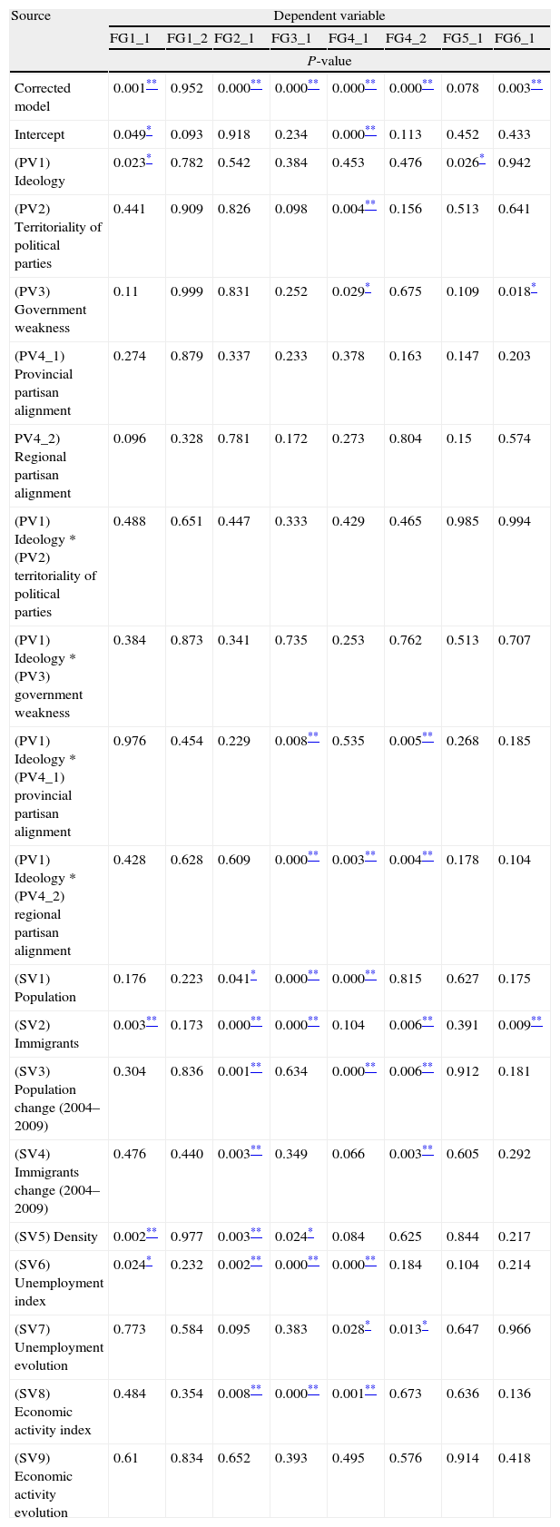
Once we identified and obtained the values of the financial dimensions and subdimensions that comprise the financial condition using the regression method, we analyzed the extent of differences based on political factors through an analysis of variance/covariance, controlling the influence of socioeconomic aspects.

We found that the normality of the residuals and the homogeneity of variances were met and the test of between-subjects effects indicates that political factors have statistically significant effects only on the volume of debt (FG1_1), on the degree of financial dependence on transfers from other institutions to perform certain services, particularly for real investments and housing and planning policies (FG4_1), and on balanced budget (FG6_1) (Table 5).

Table 5.

Tests of between-subjects effects.

Source	Dependent variable
	FG1_1	FG1_2	FG2_1	FG3_1	FG4_1	FG4_2	FG5_1	FG6_1
	P-value
Corrected model	0.001^**	0.952	0.000^**	0.000^**	0.000^**	0.000^**	0.078	0.003^**
Intercept	0.049^*	0.093	0.918	0.234	0.000^**	0.113	0.452	0.433
(PV1) Ideology	0.023^*	0.782	0.542	0.384	0.453	0.476	0.026^*	0.942
(PV2) Territoriality of political parties	0.441	0.909	0.826	0.098	0.004^**	0.156	0.513	0.641
(PV3) Government weakness	0.11	0.999	0.831	0.252	0.029^*	0.675	0.109	0.018^*
(PV4_1) Provincial partisan alignment	0.274	0.879	0.337	0.233	0.378	0.163	0.147	0.203
PV4_2) Regional partisan alignment	0.096	0.328	0.781	0.172	0.273	0.804	0.15	0.574
(PV1) Ideology * (PV2) territoriality of political parties	0.488	0.651	0.447	0.333	0.429	0.465	0.985	0.994
(PV1) Ideology * (PV3) government weakness	0.384	0.873	0.341	0.735	0.253	0.762	0.513	0.707
(PV1) Ideology * (PV4_1) provincial partisan alignment	0.976	0.454	0.229	0.008^**	0.535	0.005^**	0.268	0.185
(PV1) Ideology * (PV4_2) regional partisan alignment	0.428	0.628	0.609	0.000^**	0.003^**	0.004^**	0.178	0.104
(SV1) Population	0.176	0.223	0.041^*	0.000^**	0.000^**	0.815	0.627	0.175
(SV2) Immigrants	0.003^**	0.173	0.000^**	0.000^**	0.104	0.006^**	0.391	0.009^**
(SV3) Population change (2004–2009)	0.304	0.836	0.001^**	0.634	0.000^**	0.006^**	0.912	0.181
(SV4) Immigrants change (2004–2009)	0.476	0.440	0.003^**	0.349	0.066	0.003^**	0.605	0.292
(SV5) Density	0.002^**	0.977	0.003^**	0.024^*	0.084	0.625	0.844	0.217
(SV6) Unemployment index	0.024^*	0.232	0.002^**	0.000^**	0.000^**	0.184	0.104	0.214
(SV7) Unemployment evolution	0.773	0.584	0.095	0.383	0.028^*	0.013^*	0.647	0.966
(SV8) Economic activity index	0.484	0.354	0.008^**	0.000^**	0.001^**	0.673	0.636	0.136
(SV9) Economic activity evolution	0.61	0.834	0.652	0.393	0.495	0.576	0.914	0.418

*

Significant at 0.05.

**

Significant at 0.01.

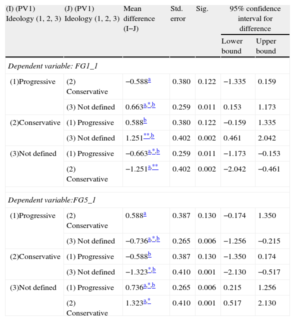
Ideology. The model reflects a significant influence of the ideology factor (PV1) on the volume of debt of the entity (FG1_1) and on the dimension of cash solvency (FG5_1) (Table 5). Specifically, the municipalities governed by political parties that have no ideology clearly positioned (not defined) as progressive or conservative have a level of debt (FG1_1) significantly lower than that of the entities that are governed by progressive parties or conservative parties (see Table 6). The mean differences between progressives and conservatives parties are not significant. The mean differences in relation to the cash solvency dimension (FG5_1) (Table 6) also show that the entities governed by the parties without an ideological option defined have higher standards of cash solvency than municipalities managed by progressive parties or by conservative parties.

Table 6.

Pairwise comparisons. Dependent variables FG1_1 and FG5_1.

(I) (PV1) Ideology (1, 2, 3)	(J) (PV1) Ideology (1, 2, 3)	Mean difference (I−J)	Std. error	Sig.	95% confidence interval for difference
					Lower bound	Upper bound
Dependent variable: FG1_1
(1)Progressive	(2) Conservative	−0.588^a	0.380	0.122	−1.335	0.159
	(3) Not defined	0.663^a^,^*^,^b	0.259	0.011	0.153	1.173
(2)Conservative	(1) Progressive	0.588^b	0.380	0.122	−0.159	1.335
	(3) Not defined	1.251^**^,^b	0.402	0.002	0.461	2.042
(3)Not defined	(1) Progressive	−0.663^a^,^*^,^b	0.259	0.011	−1.173	−0.153
	(2) Conservative	−1.251^a^,^**	0.402	0.002	−2.042	−0.461
Dependent variable:FG5_1
(1)Progressive	(2) Conservative	0.588^a	0.387	0.130	−0.174	1.350
	(3) Not defined	−0.736^a^,^*^,^b	0.265	0.006	−1.256	−0.215
(2)Conservative	(1) Progressive	−0.588^b	0.387	0.130	−1.350	0.174
	(3) Not defined	−1.323^*^,^b	0.410	0.001	−2.130	−0.517
(3)Not defined	(1) Progressive	0.736^a^,^*^,^b	0.265	0.006	0.215	1.256
	(2) Conservative	1.323^a^,^*	0.410	0.001	0.517	2.130

Based on estimated marginal means.

**

Significant at 0.01.

*

Significant at 0.05.

a

An estimate of the modified population marginal mean (I).

b

An estimate of the modified population marginal mean (J).

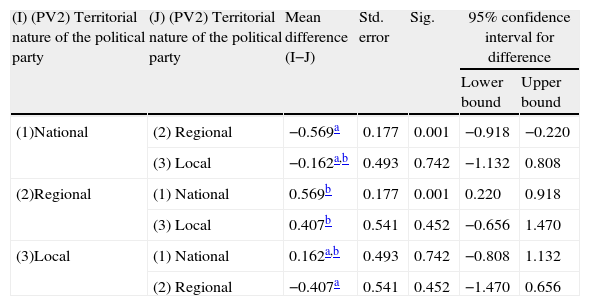
Territoriality of political parties. The territorial nature of political parties (PV2) only has a statistically significant influence on the variable (FG4_1) dependence on transfers (Table 5). Therefore, PV2 is only influencing the ratio between transfers received and transfers made, the real investments, housing and urban policies and, to a lesser extent, the implementation of policies of social protection and economic policies. Specifically, municipalities governed by regional political parties have a higher level of dependence on transfers than those governed by national parties (Table 7).

Table 7.

Pairwise comparisons. Dependent variable FG4_1.

(I) (PV2) Territorial nature of the political party	(J) (PV2) Territorial nature of the political party	Mean difference (I−J)	Std. error	Sig.	95% confidence interval for difference
					Lower bound	Upper bound
(1)National	(2) Regional	−0.569^a	0.177	0.001	−0.918	−0.220
	(3) Local	−0.162^a^,^b	0.493	0.742	−1.132	0.808
(2)Regional	(1) National	0.569^b	0.177	0.001	0.220	0.918
	(3) Local	0.407^b	0.541	0.452	−0.656	1.470
(3)Local	(1) National	0.162^a^,^b	0.493	0.742	−0.808	1.132
	(2) Regional	−0.407^a	0.541	0.452	−1.470	0.656

Based on estimated marginal means.

a

An estimate of the modified population marginal mean (I).

b

An estimate of the modified population marginal mean (J).

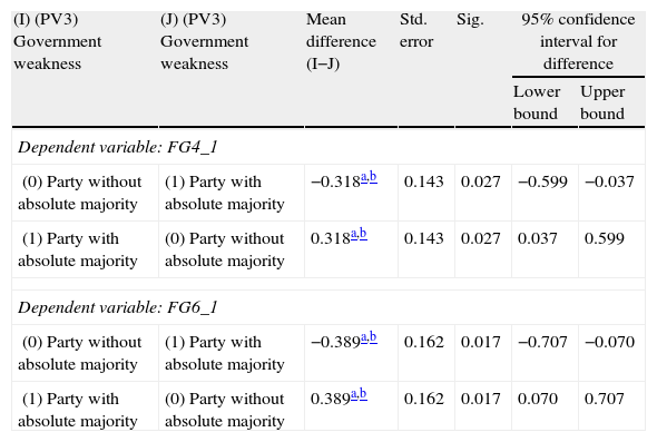
Government's weakness. The government's weakness (PV3) significantly influences the dimensions FG4_1 and FG6_1 (Table 5). The mean differences (Table 8) indicate that municipalities governed by parties that have an absolute showed a different behavior in relation to fund transfers received and transfers made, real investments, housing and urban development policies (FG4_1). The results seem to move in the opposite direction to the conclusions of Bruce et al. (2007). They note that infrastructure investments are higher when governments lack unity.

Table 8.

Pairwise comparisons. Dependent variables FG4_1 and FG6_1.

(I) (PV3) Government weakness	(J) (PV3) Government weakness	Mean difference (I−J)	Std. error	Sig.	95% confidence interval for difference
					Lower bound	Upper bound
Dependent variable: FG4_1
(0) Party without absolute majority	(1) Party with absolute majority	−0.318^a^,^b	0.143	0.027	−0.599	−0.037
(1) Party with absolute majority	(0) Party without absolute majority	0.318^a^,^b	0.143	0.027	0.037	0.599
Dependent variable: FG6_1
(0) Party without absolute majority	(1) Party with absolute majority	−0.389^a^,^b	0.162	0.017	−0.707	−0.070
(1) Party with absolute majority	(0) Party without absolute majority	0.389^a^,^b	0.162	0.017	0.070	0.707

Based on estimated marginal means.

a

An estimate of the modified population marginal mean (I).

b

An estimate of the modified population marginal mean (J).

In addition, if the ruling parties have an absolute majority, they improve the balance in budgets (FG6_1) (Table 8).

Partisan alignment. We could not find significant evidence to support the partisan alignment of the municipal governments (PV4_1 and PV4_2).

4

Conclusions

Many works in the literature have studied the effects of various political situations on public financial management. They have focused on the analysis of specific financial issues such as debt, deficits, transfers, expenses, income, or taxes, using as independent variables specific political factors, such as ideology, government weakness, political cycles, and partisan alignment. In contrast to these previous works, we have used a global concept of the financial health of public institutions, that is, the financial condition, and on this basis, we analyzed the incidence of multiple political factors.

Using a multivariate approach and a very large set of financial indicators (39) on almost all Spanish municipalities with population on over 20,000, we have identified 8 different financial dimensions or sub-dimensions within the overall concept of financial condition.

As the aim of our study was to understand the possible relationship between the essence of the policy options and all aspects of the financial condition of Spanish municipalities, we selected the most distant year of elections in order to eliminate possible effects of the electoral process.

We found that those parties that have no clear ideological position show a debt management and a short-term solvency better than parties identified ideologically as progressives or conservatives. In our study, we could not find that the municipalities governed by progressive or conservative parties differ in their financial health. Similar results were obtained by Alesina and Tabellini (1990), and Franzese (2002), and opposite results were obtained by Persson and Svensson (1989).

Our analysis of financial condition allowed us to identify a financial behavior about ratio between transfers received and transfers made, the real investments, housing and urban policies and, to a lesser extent, the implementation of policies of social protection and economic policies. This behavior is clearly influenced by the territoriality of political parties, which confirms the theory of Hearl et al. (1996) and Brancati (2008), and the government's weakness, which seems to move in the opposite direction to the conclusions of Bruce et al. (2007). They note that infrastructure investments are higher when governments lack unity, and this conclusion was confirmed by Goeminne et al. (2008) in the Flemish municipalities.

Moreover, our study confirms the government weak hypothesis in Spanish municipalities, because the municipalities in which there is no political party with an absolute majority present major fiscal imbalances (Alesina & Perotti, 1995; Roubini & Sachs, 1989). In addition, we could not verify the influence of the partisan alignment on any financial dimension, which contrasts notably with those noted by Solé-Ollé and Sorribas-Navarro (2008) and Curto-Grau et al. (2012).