Estimation of Extreme Wind Speeds by Using Mixed Distributions

Abstract

Structures are designed with the intention of safely withstanding ordinary and extreme wind loads over the entire intended economic lifetime. Due to the fact that extreme wind speeds are essentially random, appropriate statistical procedures needed to be developed in order design more accurately wind-sensitive structures. Five mixed extreme value distributions, with Gumbel, reverse Weibull and General Extreme Value components along with the Two Component Extreme Value distribution were used to model extreme wind speeds. The general procedure to estimate their parameters based on the maximum likelihood method is presented in the paper. A total of 45 sets, ranging from 9-year to 56-year, of largest annual wind speeds gathered from stations located in The Netherlands were fitted to mixed distributions. The best model was selected based on a goodness-of-fit test. The return levels were estimated and compared with those obtained by assuming the data arise from a single distribution. 87% of analyzed samples were better fitted with a mixed distribution. The best mixed models were the mixed reverse Weibull distribution and the mixture Gumbel-Reverse Weibull. Results suggest that it is very important to consider the mixed distributions as an additional mathematical tool when analyzing extreme wind speeds.

Resumen

Las estructuras son diseñadas para resistir de forma segura las cargas de viento ordinarias o extremas en el periodo de su vida útil. Debido a que las velocidades de viento son esencialmente aleatorias se requiere de procedimientos estadísticos que estimen de manera más confiable la carga por viento, para la cual una estructura trabajará eficientemente. En este trabajo se presentan cinco distribuciones de probabilidad de valores extremos mixtas, cuyas componentes son las distribuciones Gumbel, Weibull, General de Valores Extremos y TCEV para modelar velocidades extremas de viento. Los parámetros de dichas distribuciones son obtenidos por la técnica de máxima verosimilitud. Para aplicar las distribuciones mezcladas propuestas se utilizaron los registros de velocidades de viento máximo anual de 45 estaciones localizadas en Holanda, cuyas longitudes varían de 9 a 56 años. El mejor modelo univariado o mezclado fue elegido a través de un criterio de bondad de ajuste. Un 87% de las muestras analizadas se ajustaron mejor a una distribución mezclada y las mejores combinaciones fueron las de Gumbel-Weibull y la Weibull-Weibull. Los resultados sugieren que es muy importante considerar a las distribuciones mezcladas como una herramienta adicional en el análisis de velocidades de vientos extremos.

Introduction

Structures are designed with the intention of safely withstanding ordinary and extreme wind loads over the entire intended economic lifetime. The wind pressures on a structure are a function of the characteristics of the approaching wind, the geometry of the structure under consideration, and the geometry and proximity of the structures upwind. The pressures are not uniformly distributed over the surface of the structure and they can result in fatigue damage and in a probable dynamic excitation. Because of the many uncertainties involved, the maximum wind loads experienced by a structure during its lifetime, may vary widely from those assumed in design.

In terms of designing a structure for lateral wind loads the following basic design criteria need to be satisfied:

• 1)

  Stability against overturning, uplift and/or sliding of the structure as a whole.

• 2)

  Strength of the structural components of the building is required to be sufficient to withstand imposed loading without failure during the life of the structure.

• 3)

  Serviceability for example for buildings, where interstorey and overall deflections are expected to remain within acceptable limits.

The ultimate limit state wind speed is adopted by most international codes to satisfy stability and strength limit state requirements. In many codes such a speed has a return period of fifty years (Û₅₀).

The objective of wind speed frequency analysis is to obtain the most accurate estimates to any return period of occurrence through the use of probability distributions.

Much of the work in extreme value theory begins with the assumption that X₁, X₂, … , X_n are independent and identically distributed observations with some common, but unknown, distribution function F(x): The Fréchet distribution (with infinite upper tail), The Gumbel distribution (with infinite upper tail) and the reverse Weibull distribution, whose upper tail is finite (Castillo, 1988).

In the early 1970's two competing models of extreme wind speeds were widely used: the extreme value type II or Fréchet distribution and the extreme value distribution type I or Gumbel distribution. However, for long return periods the Fréchet distribution can lead to unrealistically high estimated speeds and inefficient for design purposes (Simiu et al., 1978).

In some works (Dukes and Palutikof, 1995; Simiu and Heckert, 1996; Heckert and Simiu, 1998, and Simiu et al., 2001) the Reverse Weibull distribution, based on epochal and peaks over threshold (POT) approaches, has been considered to be better in comparison to the Gumbel distribution for modeling extreme wind speeds.

In contrast, Galambos and Macri (1999) found that the assumption of bounded wind speeds and the subsequent implementation of the POT method for estimating the required parameters from wind speeds data lead to contradictions and that the Gumbel distribution is better to model extreme wind speeds. Perrin et al. (2006)also found that the Reverse Weibull distribution generates incorrect estimates of the tails of the distributions of wind speeds and of the distribution of annual maxima wind speed.

According to results obtained in those works, none of two extreme distributions (Gumbel or Reverse Weibull) can be considered better or totally adequate to model extreme wind speeds.

Simiu (2002) wrote “It is likely that better probabilistic models of extreme wind speeds could be developed if statistics of thunderstorm and large-scale storm wind speeds could be developed separately and combined in mixed distributions”. So, efforts in this direction have already been reported (Holmes and Moriarty, 1999; Dougherty et al., 2003).

In order to continue with this topic, six mixed extreme value distributions are proposed to model annual maximum wind speed samples.

Univariate extreme value distributions

In general, extreme value distributions have been widely used for fitting the distribution of extreme wind speeds. The name extreme value is attached to these distributions because they can be obtained as limiting distributions (as n → ∞) of the greatest value among n independent random variables, each having the same continuous distribution.

The general solution of the functional equation that must satisfy the extreme values has been called General Extreme Value distribution, which directly represents the Types II, and III extreme value distributions. Type I distribution results as limiting condition of the General Extreme Value distribution. Each type is characterized by the value of the shape parameter β as: Gumbel distribution β = 0, Fréchet distribution β < 0 and Weibull distribution β > 0.

The probability density function (pdf) of the Gumbel distribution is

where υ and α are the location and scale parameters, and α > 0.

The pdf of the standard Fréchet distribution is

where σ and λ are the scale and shape parameters, with σ > 0 and λ > 0.

The pdf of the Reverse Weibull distribution is

where φ and κ are the scale and shape parameters, with φ > 0 and κ > 0.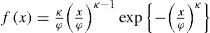

The pdf of the General Extreme Value distribution is

where ω, η and β are the location, scale and shape parameters, and η > 0.

Mixed distributions

Extreme wind speeds (EWS) have been analyzed through the use of univariate distributions. Several assumptions underlay the statistical estimate of the wind speed. The most important one that all extremes (up to return periods of 10⁴ yr) belong to the same population is hard to verify from the available short observational sets.

Van et al. (2004) noticed the existence of areas where the extreme value distribution of extratropical winds was double populated.

They demonstrated that the local wind can be caused by two meteorological systems “1” and “2” of different physical nature, each of them generating its own distribution F₁(x) and F₂(x). Then, the parent distribution F(x) is said to be mixed.

The use of a mixture of probability distributions functions for modeling samples of data coming from two populations have been proposed long time ago (Mood et al., 1974):

where p is a factor used to weight the relative contribution of each population (0 < p < 1).

Mixed Gumbel Distribution (MG)

If F₁(x) and F₂(x) of (5) are Gumbel distributions, the corresponding mixed pdf is (Raynal and Guevara, 1997):

where υ₁, α₁ and υ₂ , α₂ are the location and scale parameters for the first and second population, respectively, and p is the association parameter (0 < p < 1).

Mixed General Extreme Value Distribution (MGEV)

If F₁(x) and F₂(x) of equation (5) are General Extreme Value distributions, the mixed pdf is (Raynal and Santillan, 1986):

where ω₁, η₁, β₁ and ω₂, η₂, β₂ are the location, scale and shape parameters for the first and second population, respectively, and p is the association parameter (0 < p < 1).

Mixed Reverse Weibull Distribution (MRW)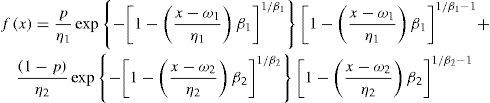

If F₁(x) and F₂(x) of equation (5) are Reverse Weibull distributions, the mixed pdf is (Escalante, 2006):

where φ₁, κ₁ and φ₂, κ₂ are the scale and shape parameters for the first and second population, respectively, and p is the association parameter (0 < p < 1).

Mixed Gumbel-Reverse Weibull Distribution (G-RW)

Assuming that first and second populations behave as Gumbel and Reverse Weibull distributions, respectively, the pdf of equation (5) yields to the five-parameter mixture model:

where υ₁, α₁ are the location and scale parameters for the first population, φ₂, κ₂ are the scale and shape parameters for the second population, and p is the association parameter (0 < p < 1).

Mixed Gumbel-General Extreme Valued Distribution (G-GEV)

Assuming that first and second populations behave as Gumbel and General Extreme Value distributions, respectively, the pdf of equation (5) yields to the six-parameter mixture model:

where υ₁, α;₁ are the location and scale parameters for the first population, and ω₂, η₂, β₂ are the location, scale and shape parameters for the first and second population, and p is the association parameter (0 < p < 1).

Two Component Extreme Value (TCEV) Distribution

The cumulative density function is (Rossi et al., 1984):

The corresponding pdf is

Estimation of parameters by maximum likelihood

Since the parameters of the mixed distributions are unknown, they must be estimated from data. The method of maximum likelihood for estimation of the parameters of the mixed extreme value distribution was selected due to its wide applicability and the efficiency features associated with it, which are not easily found in other methods of parameter estimation.

The likelihood function of n random variables is defined to be the joint density of n random variables and it is a function of the parameters. If is a random sample of a univariate density function, the corresponding likelihood function is (Mood et al., 1974):

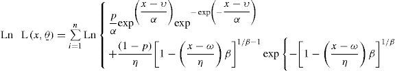
The logarithmic function will be used instead of the likelihood function because it is easier to handle. So, equation (13) is transformed:

where L is called the likelihood function; Ln is the natural logarithm; θ is the set of parameters to be estimated, and fx,θ_; is the univariate or mixed pdf.

For the case of the G-GEV distribution, equation (14) is

Due to the complexity of the mathematical expressions in (14) and the partial derivatives with respect to the parameters, the constrained multivariable Rosenbrock method (Kuester and Mize, 1973) was applied to obtain the estimators of the parameters by the direct maximization of (14).

Once obtained the parameters, the quantiles for different return periods can be estimated by solving equation (5). For the case of MG distribution:

where Û_T is the maximum extreme wind speed (in m/s) associated with T years of return period.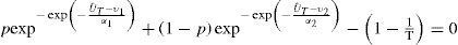

The best model can be selected based on the criterion of minimum standard error of fit (SEF), as defined by Kite (1988):

where g_i, i = 1, … , n are the recorded events; h_i, i = 1, … , n are the event magnitudes computed from the univariate or mixed distributions at probabilities obtained from the sorted ranks of g_i, i = 1, … ,n; q is the number of parameters estimated for the univariate or mixed distributions; n is the length of record, and j is the number of the analyzed station.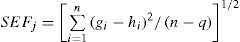

So, q = 2 for the Gumbel and Reverse Weibull distributions; q = 3 for the General Extreme Value Distribution; q = 4 for the TCEV distribution; q = 5 for the MG, MRW and G-RW distributions, and q = 6 for the MGEV distribution.

Case study

The mixed extreme value distributions were applied to model the annual maxima wind speed data gathered of the hourly potential winds computed at 45 stations located in The Netherlands (Figure 1). This country has a typical midLatitude oceanic climate with prevailing westerly winds. Winter storms are the result of differences in temperature between the polar air masses and the air in the middle latitudes in autumn and winter. These extratropical cyclones generally have less destructive power than tropical cyclones by they are able to provide damaging winds over wide coastal and inland areas.

Figure 1.

Location of wind stations used in case study

Data are available from the Royal Netherlands Meteorological Institute (KNMI). Lengths of record vary from 9 to 56 years (Table 1).

Table 1.

Some characteristics (m/s) of stations analyzed in this study

Wind station	Period of record	Mean	Standard Deviation	Minimum value	Maximum value
Arcen	1991–2004	15.3	1.2	13.8	17.7
Beek	1962–2005	17.8	2.3	12.8	23
Cabauw	1987–2004	19.1	3	14.9	25.7
Cadzand	1972–2004	20.7	2.5	17.2	26.2
De Bilt	1961-2005	16.5	2.5	10.5	22.8
De Kooy	1972–2004	21.8	2.8	18	28.8
Deelen	1961–2005	18.5	2.9	12.9	25.9
Eelde	1961–2005	18.6	2.3	15.5	24.1
Eindhoven	1960–2005	17.6	2.6	14	23.3
Europlatform	1984–2005	23.1	2.1	20.7	29.2
Gilze-Rijen	1961–2005	17.3	2.5	13.6	23.2
Heino	1991–2004	16.5	1.9	12.2	18.9
Herwijnen	1966–2004	19.1	2.9	14.2	26.7
Hoek van Holland	1962–2005	20.6	2	16.3	25.8
Hoogeven	1981–2004	17.5	2	13	20.9
Hoorn	1995–2004	20.9	1.4	19.5	24.2
Houtrib	1977–1994	20	2.7	15.9	25.9
Huibertgat	1981–2004	23.2	2.3	20.1	30
Hupsel	1990–2004	17.2	2.8	13.3	23.1
IJmuiden	1952–2005	21.4	2.1	16.9	26
K13	1983–2004	23.9	2.8	20.9	31.1
L. E. Goeree	1975–2004	21.2	2.4	17.2	26.6
Lawersoog	1969–2004	21.1	2.4	17.5	27.3
Leeuwarden	1962–2005	20.2	2.8	16.8	28.1
Lelystad	1983–2004	19	3.2	14.7	26.2
Marknesse	1990–2004	17.7	1.7	15.7	21.4
Meetpost Noordwijk	1991–2005	22.8	2	19.9	26.9
Niuew Beerta	1991–2004	19.5	2	17.1	24.1
Oosterschelde	1982–2004	21.6	2	18.2	26.4
Rotterdam Geulhaven	1981–2004	19.6	2.8	16.2	25.7
Schaar	1983–2003	20.8	1.8	18.5	25.6
Schiphol	1950–2005	20.8	2.6	15.7	28
Soesterberg	1959–2005	17.3	2.5	13.6	25.2
Stavoren-Haven	1991–2002	19.9	1.3	16.9	21.7
Terschelling	1969–1995	22.3	2	19.2	27
Texelhors	1969–2004	21.8	2.9	18	29.4
Tholen	1983–2003	19.6	2.4	15.8	24.4
Twenthe	1971–2004	16.8	2.9	12.7	23.7
Valkenburg	1982–2004	20.2	2.6	15.5	25.6
Vlissingen	1959–2005	20	2.2	16.3	25.8
Volkel	1971–2004	17.3	2.8	12.7	26.9
Wijdenes	1995–2004	19.7	2.1	16.4	22.6
Wilhelminadorp	1990–2004	19.1	2.3	16.4	24
Wownsdrecht	1996–2004	16.8	2.5	14.1	22.3
Zeistienhoven	1962–2005	19.5	2.5	14.8	26.8

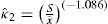
As it is known, in any of the multivariable constrained non-linear optimization techniques, global optimality is never assured. Therefore, care must be taken in order to avoid a local optimum. It is suggested to start always with a set of initial parameters (Moments estimators). For example, in Schiphol station for the case of the G-RW distribution, sample is sorted in decreasing order of magnitude and divided into two parts. The first one contains a third of the sample (association parameter p = 0.33) with a mean equal to 23.85 m/s and standard deviation equal to 1.62 m/s. With these values and by using equations (18) and (19), the initial parameters for the Reverse Weibull distribution are computed κˆ2=18.546, ϕˆ2=24.546. For the rest of the sample with a m ean equalto 19.41 m/s and standard deviation equal to 1.56 m/s, initial parameters for the Gumbel distribution are computed with equations (20) and (21), νˆ1=18.70,  αˆ1=1.214.

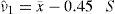
The final maximum likelihood estimators by the direct maximization of equation (14) are:

In this station the best univariate fit was obtained using the General Extreme Value distribution with a SEF = 0.320 m/s and Û₅₀ = 26.7 m/s.

In Figure 2, a graphical comparison between the empirical and fitted distributions (G-RW) is made.

Figure 2.

Empirical and fitted frequency curves for the Extreme Wind Speed at Shiphol station

The univariate and mixed return levels U(m/s) for different return periods T(years) along with the minimum value of the standard error of fit were obtained for each analyzed station. If only the univariate distributions had been considered in the wind speed frequency analysis 40% of the samples would have been better fitted with the Gumbel distribution, 56% with the General Extreme Value distribution, and 4% with the Reverse Weibull distribution.

It was possible to reduce the standard error of fit when mixed distributions were applied. 40% of samples were better fitted with the MRW distribution, and another 40% with the G-RW distribution. For instance, in station K13 with 22 years of record, the best univariate fit was obtained with the General Extreme Value distribution, SEF = 0.910 m/s and Û₅₀ = 32.7 m/s, and the best mixed fit was obtained with the MRW distribution with a SEF = 0.443 m/s and the return level reduced to Û₅₀ = 30.9 m/s, which also represents a significant difference for design purposes.

It was also seen that the reduction of the SEF was important in the cases when the analyzed sample has a short length of record. This fact represents a great advantage of the mixed distributions with reference to univariate distributions. The final values of the return levels are shown in Table 2.

Table 2.

Return levels (in m/s) for the best univariate or mixed distribution in each wind station.

	Final					Return	Period	(years)
Wind station	Model	2	5	10	20	50	100	500	1000	5000	10000	SE
Arcen	G-RW	15.1	16.3	17.2	17.6	17.9	18.2	19.4	19.9	21.2	21.7	0.258
Beek	MRW	17.3	20.0	21.0	21.7	22.3	22.7	23.4	23.7	24.1	24.3	0.273
Cabauw	G-RW	18.4	21.8	24.0	25.0	25.9	26.4	27.5	28.3	31.0	32.1	0.44
Cadzand	G-RW	20.2	23.2	24.3	25.1	25.8	26.2	27.1	27.5	29.0	29.9	0.313
De Bilt	MRW	16.3	18.0	20.6	21.7	22.3	22.6	23.2	23.3	23.7	23.8	0.351
De Kooy	G	21.4	23.8	25.5	27.1	29.1	30.6	34.2	35.7	39.2	40.7	0.380
Deelen	G-RW	18.3	20.9	22.4	23.7	25.2	26.4	29.0	30.1	32.7	33.9	0.374
Eelde	G-RW	17.9	20.4	22.1	23.3	24.4	25.0	26.2	26.6	27.6	28.1	0.295
Eindhoven	G-RW	17.2	20.1	21.7	22.7	23.8	24.5	26.9	28.1	31.1	32.3	0.301
Europlatform	MG	22.5	24.7	26.1	27.3	28.8	29.9	32.5	33.6	36.1	37.2	0.491
Gilze-Rijen	G-RW	16.9	19.4	21.1	22.4	23.7	24.5	26.7	28.0	30.8	32.1	0.363
Heino	G-RW	16.8	18.0	18.5	18.9	19.3	19.7	22.2	23.6	26.8	28.2	0.521
Herwijnen	G	18.6	21.3	23.1	24.8	27.1	28.7	32.6	34.3	38.1	39.8	0.300
Hoek van Holland	MRW	20.5	22.1	23.3	24.2	25.0	25.4	26.2	26.5	27.0	27.2	0.229
Hoogeven	RW	17.7	19.1	19.8	20.3	20.8	21.1	21.7	22.0	22.4	22.6	0.285
Hoorn	G-RW	20.4	21.4	23.7	24.2	24.3	24.3	24.4	24.4	25.0	25.4	0.519
Houtrib	MRW	19.6	22.2	24.2	25.2	26.1	26.5	27.4	27.6	28.2	28.4	0.445
Huibertgat	MRW	22.6	24.9	26.9	28.1	29.2	29.8	30.9	31.3	32.0	32.3	0.453
Hupsel	MRW	16.5	19.9	21.5	22.4	23.1	23.5	24.2	24.5	24.9	25.1	0.615
IJmuiden	MRW	21.0	23.4	24.5	25.1	25.6	25.9	26.4	26.6	27.0	27.1	0.201
K13	MRW	23.4	24.7	29.5	30.4	30.9	31.2	31.5	31.7	31.9	32.0	0.443
L. E. Goeree	MRW	21.0	23.3	24.9	25.6	26.2	26.5	27.1	27.3	27.7	27.9	0.299
Lawersoog	G-RW	20.6	22.8	24.7	26.2	27.4	28.1	29.3	29.8	31.5	32.5	0.312
Leeuwarden	MRW	19.7	21.8	25.0	26.3	27.3	27.9	28.8	29.1	29.7	29.9	0.469
Lelystad	MRW	18.5	20.8	24.5	25.6	26.5	26.9	27.7	28.0	28.5	28.6	0.522
Marknesse	MRW	17.3	19.4	20.3	20.9	21.4	21.8	22.3	22.5	22.9	23.0	0.352
Meetpost Noordwijk	G-RW	22.5	24.4	26.0	26.7	27.6	28.3	29.7	30.3	31.7	32.3	0.383
Niuew Beerta	MRW	19.2	20.5	23.0	23.7	24.1	24.4	24.7	24.8	25.0	25.1	0.415
Oosterschelde	G	21.3	23.0	24.2	25.4	26.8	27.9	30.5	31.6	34.1	35.2	0.360
Rotterdam Geulhaven	G-RW	18.8	21.8	24.1	25.4	26.4	27.0	28.0	28.4	29.5	30.3	0.470
Schaar	G-RW	20.4	22.2	23.5	24.8	26.4	27.7	30.5	31.6	34.4	35.6	0.249
Schiphol	G-RW	20.5	23.4	24.1	25.6	27.6	29.1	32.7	34.2	37.7	39.2	0.285
Soesterberg	TCEV	16.9	19.2	20.7	22.2	24.2	25.6	29.0	30.5	33.9	35.4	0.300
Stavoren-Haven	G-RW	19.9	20.8	21.4	22.0	22.8	23.3	24.6	25.2	26.5	27.0	0.323
Terschelling	G	21.9	23.8	25.0	26.2	27.7	28.8	31.5	32.6	35.2	36.3	0.350
Texelhors	MRW	21.4	23.3	26.7	28.3	29.4	30.0	30.9	31.1	31.7	31.9	0.471
Tholen	MRW	19.4	21.1	23.7	24.1	24.4	24.5	24.7	24.7	24.8	24.9	0.311
Twenthe	MGEV	16.1	19.7	21.1	22.1	23.0	23.5	24.2	24.5	24.8	24.9	0.305
Valkenburg	G	19.8	22.3	24.0	25.6	27.7	29.2	32.8	34.3	37.9	39.4	0.470
Vlissingen	MRW	19.8	21.2	23.6	24.9	25.5	25.7	26.2	26.3	26.6	26.6	0.236
Volkel	MRW	16.8	19.1	21.8	23.4	25.0	25.9	27.5	28.1	29.3	29.7	0.527
Wijdenes	RW	19.9	21.4	22.0	22.5	23.0	23.3	23.9	24.1	24.6	24.7	0.572
Wilhelminadorp	MG	18.6	21.0	22.1	23.1	24.4	25.4	27.5	28.5	30.7	31.6	0.506
Wownsdrecht	G-RW	16.5	17.8	21.2	23.3	25.2	26.5	29.3	30.5	33.3	34.5	0.809
Zeistienhoven	G-RW	19.1	20.6	23.2	24.8	26.5	27.8	30.6	31.8	34.6	35.7	0.312

Conclusions

The general objective of this study is to show how the mixed distributions can be applied to model extreme wind speeds.

Five mixed extreme value distributions, with Gumbel, Reverse Weibull, and General Extreme Value components along with the Two Component Extreme Value distribution were used to model extreme wind speeds. The maximum likelihood estimators of the parameters were obtained numerically by using the multivariable constrained Rosenbrock optimization algorithm, which worked out very well in all cases.

Results have shown that there exists a reduction in the standard error of fit when estimating the parameters with mixed distributions instead of its univariate counterpart, and differences between univariate and mixed design events can be significant as return period increases. 87% of samples were better fitted with a mixed distribution.

In 34 analyzed samples at least one of the components of the mixed distribution is the Reverse Weibull distribution. Besides, the final return levels were not observed like unrealistic design events even for long return periods.

Results suggest that it is very important to consider the mixed distributions as an additional mathematical tool when analyzing extreme wind speeds.