Output gaps and stabilisation policies in Latin America: The effect of commodity and capital flow cycles

Abstract

We provide a measure of the output gap that filters out the impact of the commodity and net capital inflows booms for Latin American countries. These two factors temporarily boost output and so are likely to push up estimates of potential growth in the region to unrealistic levels, thereby resulting in an underestimation of the output gaps during the upswing of the commodity cycle. We also shed light on the interaction between the two components. The results show that commodity prices have been the dominant factor explaining deviation of activity from sustainable levels. A timely consideration of these factors could prevent a procyclical fiscal policy bias in the region.

Resumen

Se proporciona una medida de la brecha de producción que filtra el impacto del auge de materias primas y flujos de capitales en los países latinoamericanos. Estos dos factores potencian temporalmente la producción y por tanto tienden a inflar las estimaciones de crecimiento potencial hasta niveles excesivos, lo que resulta en una subestimación de las brechas de producción durante la fase ascendente del ciclo de las materias primas. También se arroja luz acerca de la interacción entre ambos componentes. Los resultados muestran que los precios de las materias primas constituyen el factor dominante para explicar la desviación de la actividad económica con respecto a niveles sostenibles. La consideración de estos factores podría evitar un sesgo fiscal procíclico en la región.

1

Introduction

In the last decade Latin America has experienced a long period of sustained growth and unprecedented economic and financial stability. The parenthesis represented by the global financial crisis was short-lived and did not spawn trouble in the domestic financial sector. Moreover, the swift recovery of the region fed the perception that countries had turned the page and they could sustain higher rates of growth than in the past.

A much improved macroeconomic framework, a reduction in financial vulnerability and a broadening of the domestic demand base were seen as key factors of that change. The benign external environment was also given some credit: the loose global financing conditions before and after the crisis, which fostered large capital inflows and the sustained increase of commodity demand and prices helped. Resource-rich Latin American countries with low saving rates – and thus heavy dependence in external financing – were especially favoured by this set of circumstances.

To illustrate this point, Fig. 1 displays the evolution of GDP growth, net capital inflows as a percentage of GDP and the (country-specific) growth rate of commodity prices since the nineties for a set of Latin American countries. The upward trend in commodity prices since the beginning of last decade was briefly interrupted during the global recession but resumed its two-digit growth shortly afterwards. However, after mid-2011 commodity prices plummeted. The evolution of net capital inflows has certain similarities: they increased strongly in the early 2000s, recovered rapidly after the global financial crisis and moderated towards the end of the sample. A certain co-movement is visible among the three variables, in particular during the last decade.

Fig. 1.

Input variables.

¹ Weighted averages based on GDP and PPP exchange rates for Brazil, Chile, Colombia, Mexico and Peru. For Peru, data until Q4 2013. ²Country specific commodity price index calculated using 3 digits exports weights for SITC Rev. 3. ³As a share of GDP.

Sources: Bloomberg; Datastream; IMF, Balance of Payments; Primary Commodity Prices; UN Comtrade; UNCTAD Statistics; World Bank; national data; BIS calculations.

The sharp slowdown in growth in most countries of the sample has come as a surprise to many. The co-movement between the variables in Fig. 1 suggests that not only the current disappointing growth but also the robust recovery from the crisis is closely linked to the reversal in the external conditions. The fall in commodity prices, which was not anticipated, has severely affected growth prospects: it is remarkable to see in Fig. 2 how growth forecasts have been systematically revised downwards in the region, coinciding with the reversal in commodity prices.

Fig. 2.

GDP growth forecasts evolution for Latin America.¹

This figure can be seen in colour in the electronic version.

¹Weighted average based on PPP exchange rates for Argentina, Brazil, Chile, Colombia, Mexico and Peru.

Source: IMF, World Economic Outlook.

Let us take for instance Brazil, a country whose share of commodity exports has averaged more than 60% in the last decade. Fig. 3 shows the strong positive correlation between changes in commodity prices and growth rates in Brazil. The correlation is even stronger with the changes in the growth forecasts, suggesting that economic performance is perceived to be closely associated with the evolution of commodity prices.

Fig. 3.

Correlation of commodity prices and GDP growth in Brazil from 2003 to 2016.¹

¹Country specific commodity price index calculated using 3 digits exports weights for SITC Rev. 3. ²Revisions to forecast is defined as revt=yt,m−yt−1,m, where y is the forescast for year t made in month m. Commodity prices are brought forward one period since when forecast is made it is already observed.

Sources: Bloomberg; Consensus economics; Datastream; IMF Primary Commodity Prices; UN Comtrade; UNCTAD Statistics; World Bank; national data; BIS calculations.

As a matter of fact, expectations of long-term growth in Latin America, boosted by the boom in commodity prices, have been scaled back. The IMF's five-year ahead forecasts, which can be seen as a proxy for the long-term expectations of potential growth, have been revised down from 4% to 3%.

There is a growing acknowledgement that long-term growth expectations in Latin America have been boosted by those extraordinary conditions is settling. This implies that the sustainable rate of growth in normal circumstances is perceived as lower than in the post-crisis recovery, and that the output gaps during the bonanza were underestimated.

This paper explores how to convey the extraordinary factors which have boosted growth in Latin America in the estimation of potential output and, hence, the output gaps.

The concept of potential output is an elusive one, relating to the rate of growth that a certain economy can attain without the insurgence of adverse side effects that may compromise future economic performance. The output gap – namely the difference between actual and potential output – is therefore a measure of the amount of slack or overheating at a certain point in time. As such, the notion of potential output is intertwined with that of sustainable growth. The sense in which sustainability should be interpreted varies depending on the specific approach taken.

One strand of approaches is based on production functions: potential output is expressed as a function of the input factors in the production process (capital, labour and technology). Accordingly, output above potential indicates that production factors are being overused, which could compromise future economic growth. The most widespread approach however relates sustainability to inflation: rising prices are interpreted as a sign of unsustainable growth. However, the structural changes in the relationship between inflation and unemployment in recent decades and the difficulties to estimate ‘sustainable’ – or equilibrium – employment rates has eroded the reliability of this approach.

Other approaches are entirely data-driven. For instance, the Hodrick–Prescott filter and other univariate time series filters (Baxter & King, 1999; Christiano & Fitzgerald, 2003). In recent times, there have been several attempts, through this filtering approach, to correct the contamination of the estimated output gaps from the factors that may presage unsustainable growth other than inflation (see Alberola, Estrada, & Santabarbara, 2014 and Benes et al., 2010 among others). A particularly relevant addition to the literature is the incorporation of financial cycles into the estimation of the output gaps. The focus on the relationship between financial cycles and business cycles has a long tradition in the literature, but it has mushroomed after the crisis (see Borio, 2012; Claessens, Kose, & Terrones, 2011; Rabanal and Taheri, 2015). Borio, Disyatat, and Juselius (2013, 2014) propose to include financial cycle considerations in the estimation of the output gap by correcting the HP filter with variables associated to the financial cycle, such as the credit growth and the house prices.

The approach by Borio et al. (2013) has been applied to Latin American countries by Amador, Gomez, Ojeda, Jaulin, and Tenjo (2016) and to EMEs in general by Grintzalis, Lodge, and Manu (2016). In this paper, we apply a similar approach, but focus on alternative gauges of unsustainable growth that may be more relevant for Latin American economies. A first alternative is net capital flows: a bonanza of foreign investment is likely to boost demand and growth in the recipient country, but when financial conditions in source countries tighten the flows may reverse, thereby dragging on growth. There is a very large literature linking the sharp economic cycles in the region to the boom and busts of capital flows, the so-called “sudden stops”: Edwards (2004), Kaminsky, Reinhart, and Vegh (2005), Calvo and Talvi (2005).

Another common feature of the Latin American economies under study is the importance of commodities (see for instance, Céspedes & Velasco, 2012). Booms in commodity prices tend to raise real GDP in the short term by increasing the value and production of a key production factor in the economy (natural resources) and lifting the demand for ancillary goods and services. But it is an open question how far such booms raise potential growth in the longer term. By attracting capital and increasing investment in the resource sector, booms may raise potential output. And this may provide financial resources which could be in turn used to increase investment in other sectors of the economy. However, the so-called Dutch disease (Corden, 1984) operates in the opposite direction. The positive terms of trade (with the corresponding real exchange rate appreciation) and income shock associated with commodity booms shift production out of non-commodity tradables and into the non-tradable service sectors, with lower relative productivity. If the manufacturing base of the economy – the main non-commodity tradable – is reduced in a permanent way, potential growth can be reduced, too, as the tradable sector usually enjoys higher productivity levels and growth. Furthermore, commodity booms can catalyse waves of capital inflows and high demand of credit, on the basis of improved growth prospects, implying a linkage with the financial cycle too.

So, to assess potential output and diagnose the amount of economic slack at a given point in time, the status of international commodity prices should be taken into account. If one fails to consider the cyclical nature of commodity prices and assumes that their level during an upswing phase is going to last, the assessment of potential economic growth will be excessively optimistic.

By following this approach we obtain a measure of the output gap which is neutral to commodity prices and financial inflows. In other words, we aim to purge the output gap of the boosting/depressing effects that these factors may play.

Our results suggest that commodity prices are a more determinant booster of the cycle than net capital flows. The resulting output gaps, adjusted for commodity prices and (when relevant) capital inflows, are between one and three percentage points of GDP higher compared to standard univariate filters. For instance, while the standard approach yielded gaps of up to 1.5 pp of GDP in the recovery, the output gap with the adjusted filter reaches up to 5 pp and in all countries surpasses the 3 pp at some point. For the regional aggregate the peak of the output gap is 3.5 pp, compared with 1 pp of the usual method. When we take the whole upswing of the commodity cycle, this divergence also appears in most countries prior to 2008. The implied differences in potential output are also large. At the peak of the divergence the level of estimated potential output is between 2.2% and 4.8% (2.4% for the regional aggregate). These differences have narrowed in the last years, after commodity prices have fallen and capital inflows have moderated.

The results are maintained when, instead of usual ex-post estimates, we compute the real time estimates, that is, recursively estimating the output gap by adding new observations. Real time computation of output gaps comes closer to actual policymaking, therefore we use them to assess the policy implications of our analysis. Acknowledging that output gaps had been higher during the expansionary phase would have led to more prudent monetary and fiscal policies. This is particularly relevant for the analysed countries, as the commodity cum capital inflows cycles introduce an additional procyclical bias into monetary policy, through their impact on exchange rates.

The paper is structured as follows: the next section describes the data and performs a preliminary analysis to reveal some of the key relations among the variables. Section 2 explains the empirical approach and section 3 shows the main results. In section 4 we present a policy discussion based on the comparison between the real time adjusted output gaps and those considered by the economic authorities. Section 5 concludes.

2

Data and descriptive statistics: the commodity-capital flows interactions

We estimate the adjusted GDP gap using a data set of three variables: real GDP, country-specific commodity prices, and capital inflows (gross and net). Countries under scrutiny are Brazil, Chile, Colombia, Mexico and Peru, and we consider a sample ranging from 1981 to 2014, at quarterly frequency.

For real GDP we use national sources and data covers from Q1 1981 to Q1 2015.¹ Real GDP is seasonally adjusted and it is also annualised using a four-quarter moving sum.

For data on financial flows, we construct the series of gross capital flows by foreigners (inflows) and residents (outflows) as a share of GDP using both annual and quarterly data from the financial account in Balance of Payments (BoP) of the IMF.² Gross financial inflows (outflows) are defined as the sum of external liabilities (assets) comprising foreign direct, portfolio and other investment; we exclude monetary authorities’ holdings. The series of net inflows are constructed as the difference between gross financial inflows (liabilities) and gross financial outflows (assets). For each country we use four-quarter cumulative net inflows, scaled by nominal GDP (from World Economic Outlook, IMF). Annual data is linearly interpolated and joined to form quarterly figures in cases where only annual data are available.³

As the goal of the analysis is to compute output gaps, the choice of net capital flows for the exercise appears as more appropriate as this variable is expected to have a closest link to demand than gross inflows.⁴ Only results using net capital inflows are reported in what follows.

Data show a distinct behaviour among countries when it comes to net inflows (see Fig. 1). On the one hand, we observe that for Chile, net inflows have fallen 3.4 pp of GDP from 1990 to 2014. For the same period we see an increase of 4.3, 5.7, 3.4 and 5.0 pp of GDP for Brazil, Colombia, Mexico and Peru, respectively. Only Chile showed a decrease of 1.6 pp from 2003 to 2014 while the rest experienced an increase, in particular Brazil and Colombia (6.4 and 4.6 pp, respectively).

We use the country-specific commodity price indices (expressed in US dollars) developed by Kohlscheen, Avalos, and Schrimpf (2016). This is a weighted average of a basket of 83 commodity prices and commodity trade exports using 3-digit SITC Rev.3. The number of commodity prices used is based on the availability of data.⁵ Commodity trade export shares act as weights; therefore we use the average of exports between 2004 and 2013. Prices are deflated by the U.S. consumer price index. Finally, we calculate annual percentage changes for each country.

With respect to the main commodity exports by each country, most countries in the sample have an export structure which is highly concentrated on a particular product, except for Brazil, with a significant share of iron ore and agricultural products (soybean, sugar cane, coffee). Some countries in the sample are mainly metal exporters, such as Chile (copper) and Peru (copper and gold), whereas Colombia and Mexico are oil exporters. Metal exporters have roughly maintained the share of metal exports in total exports of goods since the 1990s. However, in the case of Colombia, oil exports nearly doubled since early 1990s to 40% of total exports in 2015, whereas they dropped to only 5% in Mexico.⁶ From Fig. 1 we observe that commodity export prices have diverged among countries. For example, the Brazilian commodity price index has experienced a fall between 1990 and 2014 of around 10%, while the rest have seen their prices grew from 20% to 46%. However, for the most recent period (2003–2014) all countries display large increases (110%, 109% 87%, 74%, and 38% for Chile, Peru, Colombia, Mexico and Brazil, respectively). In our analysis, we take the natural logarithm of real GDP. As in Borio et al. (2013), we adjust net inflows and country-specific commodity prices using Cesàro averages.⁷ In the case of net inflows we subtract its Cesàro average directly on the levels, while for commodity prices on the annual growth rate. This de-meaning process implies that the explanatory variables are allowed to display a linear trend in levels.⁸

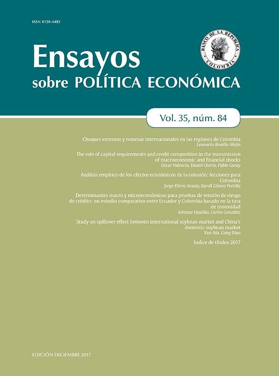
A first investigation into the data is to compute the correlations between commodity prices and net capital inflows, as displayed in Table 1. Contrary to our expectations, both variables are only strongly and positively correlated in some cases. For the whole period only Brazil fits the prior for the whole and the second part of the sample (2003–2014) and Peru and Chile (at 10% significance) for the first part of the sample. In more cases, the correlation is negative and significant, like Mexico and Chile for the whole sample commodity prices and capital flows are not strongly related overall. The exception is Brazil and some periods in other countries. As a matter of fact, the correlation is negative in several countries/periods. By contrast, the correlations between GDP growth and commodity prices tend to be positive and statistically significant, and seems to have strengthened over time. The correlation between net inflows and GDP growth is also strongly significant on historical periods, but has somehow weakened over time.

Table 1.

Country specific commodity prices and net inflows correlation.^a

	Commodity prices and net inflows			Commodity prices and GDP growth			Net inflows and GDP growth
	1	2	3	1	2	3	1	2	3
Brazil	0.28^***	0.01	0.35^**	0.56^***	0.53^***	0.62^***	0.29^***	0.23	0.35^**
Chile	−0.42^***	0.24^*	−0.58^***	0.01	−0.1	0.31^**	0.3^***	0.47^***	−0.1
Colombia	−0.01	0.03	−0.27^*	0.25^**	0.01	0.38^***	0.4^***	0.32^**	0.26^*
Mexico	−0.21^**	−0.35^**	−0.03	0.1	−0.11	0.37^***	0.26^***	0.32^**	0.1
Peru^b	0.02	0.36^**	−0.1	0.37^***	0.6^***	−0.01	0.53^***	0.7^***	0.55^***

Sample 1: 1990 to 2014; sample 2: 1990 to 2002; sample 3: 2003 to 2014.

a

For the country specific commodity prices, we use annual growth rates.

b

For Peru, data starts in Q4 1991 and ends in Q4 2013.

*

Significant at 10%.

**

Significant at 5%.

***

Significant at 1%.

To further illustrate the dynamics of the linkages between the relevant variables we resort to a simple VAR. The VAR is built around the idea of an international bloc featuring, in this order, the (country-specific) commodity price index, the Fed funds rate and the VIX. The international bloc is followed by two domestic variables: the real effective exchange rate and net financial inflows. The recursive identification scheme is loosely based on a slow-to-fast criterion, as it is customary practice.⁹ So, commodity prices are driven by an exogenous shock process to which US monetary policy is assumed to respond instantaneously. Net inflows are ordered last, which means we remain agnostic on exclusion restrictions and allow them to respond contemporaneously to the shocks to all other variables. The VAR is estimated for each country using quarterly data from 1994 Q1. Due to the relatively short sample size compared to the number of variables, we could only include two lags.

Selected results are summarised in Fig. 4. The yellow bars in the graph display the impulse response of the net inflows to one positive standard deviation shock to commodity prices; a dashed pattern implies non-significance. The graph also represents the response of the exchange rate to commodity prices and net inflows. The response of net inflows to commodity prices is positive and significant for Brazil and Peru, signalling that higher commodity prices attract financial inflows. In the rest of countries it is non-significant.¹⁰ The response of the exchange rate to commodity price shocks (red bars) is strong and significant in all cases, implying an appreciation following a positive shock. Remarkably, the exchange rate (blue bars) depreciates in some cases as a response to a positive shock to net inflows, and this effect is statistically significant in the case of Chile and Peru.

Fig. 4.

Responses to commodity prices and capital inflows shocks.¹

¹Response to Cholesky one positive s.d. innovations. Negative exchange rate movements indicate appreciation. ²Responses in per cent. ³Responses in percentage points.

Source: Author's estimations.

3

The empirical approach

To empirically assess the role that commodity prices and financial inflows may have in affecting estimates of the output gap, we resort to the methodology recently proposed by Borio et al. (2013, 2014), the so-called finance-neutral (FN) output gap. The starting point is the state-space representation of the popular HP filter:

where y_t is (log) real GDP and * denotes its potential (unobserved) level. It is commonplace to calibrate the variances of the error terms so that their ratio (the so-called signal-to-noise ratio) is equal to 1600, which roughly corresponds to a business cycle of about eight years.

Borio et al. (2013) propose to augment (2) with a set of observed variables that are capable of accounting for output fluctuations around potential. Equation (2) is therefore rewritten as:

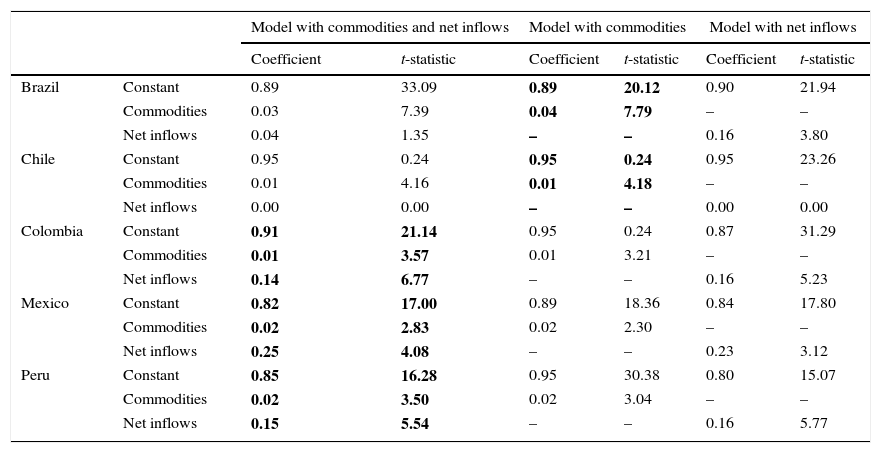
where x_t is a vector containing additional explanatory variables. Borio et al. (2013) propose setting the signal-to-noise ratio so that the relative volatility of the business cycle around potential is the same as in the standard HP filter:

As shown by Fernández-Amador, Gächter, and Sindermann (2016), the trend specification is crucial to determine the amplitude of output fluctuations. Here we stick to Borio et al. (2013), and we calibrate the trend properties to those of the HP filter to facilitate comparisons.

Borio et al. (2013) suggest that the explanatory variables should be financial factors that can account for above-potential growth experienced during financial booms. The approach is however more general, as x_t can in principle contain any variable that embeds useful information on the slack/tightness of the economic landscape. In a companion paper, Borio et al. (2014) argue for example that at the current juncture, inflation does not embed relevant information for major advanced economies, and therefore estimates of the output gap that hinge on the Phillips curve may be misleading. As anticipated in the introduction, we will instead focus on financial inflows and commodity prices as explanatory variables.¹¹

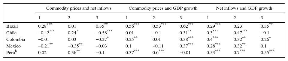
4

Results

The first step of our empirical analysis relates to model selection. For each country, we estimated models featuring both explanatory variables (commodity prices and net inflows), as well as one variable at the time.¹² Results are presented in Table 2 and differ across countries. In the first column, both variables are used in the filter. For Brazil, capital inflows are non-significant, as in Chile. In the rest of countries, both variables retain a high degree of significance. When the model is re-estimated using commodities alone (second column), we observe that all countries show significant results. By contrast, net inflows alone (third column) are significant for all countries but Chile.

Table 2.

Results from estimated models.

		Model with commodities and net inflows		Model with commodities		Model with net inflows
		Coefficient	t-statistic	Coefficient	t-statistic	Coefficient	t-statistic
Brazil	Constant	0.89	33.09	0.89	20.12	0.90	21.94
	Commodities	0.03	7.39	0.04	7.79	–	–
	Net inflows	0.04	1.35	–	–	0.16	3.80
Chile	Constant	0.95	0.24	0.95	0.24	0.95	23.26
	Commodities	0.01	4.16	0.01	4.18	–	–
	Net inflows	0.00	0.00	–	–	0.00	0.00
Colombia	Constant	0.91	21.14	0.95	0.24	0.87	31.29
	Commodities	0.01	3.57	0.01	3.21	–	–
	Net inflows	0.14	6.77	–	–	0.16	5.23
Mexico	Constant	0.82	17.00	0.89	18.36	0.84	17.80
	Commodities	0.02	2.83	0.02	2.30	–	–
	Net inflows	0.25	4.08	–	–	0.23	3.12
Peru	Constant	0.85	16.28	0.95	30.38	0.80	15.07
	Commodities	0.02	3.50	0.02	3.04	–	–
	Net inflows	0.15	5.54	–	–	0.16	5.77

Bold values correspond to the chosen model for the empirical results.

Based on these results, we retain as baseline model the commodities-only model for Chile and Brazil, and the two-variable model for Colombia, Mexico and Peru, that is, the shaded specification in Table 2. In Fig. 5, we compare the estimated output gap generated by the baseline models (blue lines) with that of the HP filter (red lines).

Fig. 5.

GDP gaps for Latin America.¹

¹Computed according to the methodology of C. Borio, P. Disyatat and M. Juselius, “A parsimonious approach to incorporating economic information in measures of potential output”, BIS Working Papers, no. 442, February 2014. The dynamic output gap equation is augmented with net inflows and country-specific commodity prices. For Brazil and Chile, only commodities prices are used to adjusted the Hodrick–Prescott filter. For Colombia, Mexico and Peru, net inflows are also included in the adjustment. ²Weighted averages based on GDP and PPP exchange rates for Brazil, Chile, Colombia, Mexico and Peru. For Peru, data until Q4 2013.

Sources: Bloomberg; Datastream; IMF, Balance of Payments; Primary Commodity Prices; UN Comtrade; UNCTAD Statistics; World Bank; national data; BIS calculations.

The first difference that stands out is that, while the dynamics of the gaps is broadly similar, adjusting for commodity prices and net inflows produces level shifts that often lead to substantially higher output gaps at times when these two variables are buoyant.

This is the case from 2002 on in countries like Chile – buoyed by high cooper prices – and Brazil. After the financial crisis and the recovery in commodities and inflows, a widening output gap appears in all countries, and the difference with the simple HP filters also opens up. The magnitude of the adjusted output gaps and the difference with the HP-based gaps differ among countries. The adjusted output gap reaches a maximum of over 6 percentage point of GDP in Chile before the crises, and this is a difference of 4 percentage points relative to the HP gaps. Brazil and Colombia also display large positive output gaps, with a peak of around 4 percentage points of GDP and also substantial differences with the HP gaps. In Mexico and Peru the difference between the adjusted and the simple HP only appears in the last years and it is of a lower order, peaking at around 2% of GDP. For the region weighted average the picture is similar, with a peak of around 4 percentage points of GDP after the crisis and a maximum difference or around 3% of GDP with the simple HP after the crisis.

In recent years, the gaps have tended to narrow, but the adjusted gap has become negative only in Brazil, while the HP gaps have closed or become negative in all countries. This means that the perception of a change of sign in the output gap is dispelled when the adjusted filter is used. This also applies to the regional average.

How do these results translate into potential output? The level and rate of growth of potential output is unobservable, but it can be simply derived by adding the (adjusted or simple) output gap to the observed level of output. Using the adjusted or the simple output gap yields different levels of potential output and potential growth. So, the relevant comparison is that difference. If the adjusted output gaps is persistently higher than HP output gaps, the level of potential output derived from the adjusted gaps would be lower, and vice versa. Note that a positive divergence between the output gaps is not immediately reflected in a lower level of potential output, as this depends on the accumulated divergence. By the same token, such divergence does not imply a lower rate of growth, as this depends on the changes in the divergence.

Fig. 6 translates Fig. 5 into levels: we show the evolution of the potential output levels and compare it with actual output. We take 2002 as a starting point, since it is a year in which both estimates were relatively similar in most countries. This allows to visualise the divergent trajectory of potential output under the two different estimation approaches. The differences are significant, in most countries and for Latin America as a whole. For instance, for Chile the level of potential output estimated by Hodrick–Prescott is up to four percentage points higher than the adjusted potential output (an annual difference of potential output growth of 0.3 pp between 2002 and 2010). The pattern is similar in Brazil (peak of 2.5%). For the aggregate of Latin America the range is between 1.9% and 2.4%, implying a difference of annual potential growth of around 0.2%.

Fig. 6.

Actual, potential and adjusted potential GDP.

¹Weighted average based on GDP and PPP exchange rates for Brazil, Chile, Colombia, Mexico and Peru.

Sources: National data; authors’ calculations.

The output gaps presented have been estimated taking into account the whole sample (ex-post estimates). It is convenient to compute the output gaps in real time, i.e. taking into account the information available at a given point in time. In our case, real times estimates for the last part of the sample are obtained by extending the initial sample of 1981–2004, adding additional quarters starting in Q1 2005, and estimating the output gaps at each moment in time.

On the one hand, real time output gaps allow to assess whether the adjusted gaps offer a more precise view of the actual cyclical position of the economy than simple HP gaps, when compared with the ex-post computations. On the other hand, policy decisions are made based on current developments and the forecasts of the future based on the information set currently available. Therefore, policy discussions have to be based on real-time estimates.

A well-known problem of statistical filters like the HP is their poor performance in real-time, due to the so-called endpoint problem. The HP filter is two-sided, so towards the end of the sample it is increasingly reliant on missing observations that have to be forecast somehow. So, it can happen that an overheating of the economy is recognised only ex-post, as sufficient observations become available, but not in real-time, which is precisely when policymakers would need to act. Borio et al. (2013) show that their finance-neutral filter provides a better performance in real-time, as conditioning on financial developments mitigates the end-point problem.

This appears to be the case, in most cases, also for our commodity- and inflows-neutral filter. In Fig. 7, we compare ex-post (solid lines) and real-time (dashed lines) estimates provided by the commodity- and inflows-neutral and the HP filter for the period 2003–2014. The real-time performance of the HP filter is particularly poor for Brazil, where the HP filter fails to recognise that the economy was overheating after 2011. On the contrary, the estimates of the adjusted filter seem to be more stable in real-time. For the other countries the differences between real-time and ex-post estimates are similar, but, again, in all case the HP filter fails to identify large output gaps after the Great Recession, while the adjusted filter does. If anything, the adjusted filter identifies in real-time even higher output gaps in the post crisis phase, as is clearly seen in the aggregate for Latin America.

Fig. 7.

Comparison of unadjusted and adjusted (ex-post and real time) GDP gap.^1,2

¹ Computed according to the methodology of C. Borio, P. Disyatat and M. Juselius, “A parsimonious approach to incorporating economic information in measures of potential output”, BIS Working Papers, no. 442, February 2014. The dynamic output gap equation is augmented with net inflows and country-specific commodity prices. For Brazil and Chile, only commodities prices are used to adjusted the Hodrick–Prescott filter. For Colombia, Mexico and Peru, net inflows are also included in the adjustment. ²Real time estimation started in Q1 2005 and it was estimated quarter by quarter until Q4 2014 (except for PE, which ends in Q4 2013). ³Weighted averages based on GDP and PPP exchange rates for Brazil, Chile, Colombia, Mexico and Peru. For Peru, data until Q4 2013.

Sources: Bloomberg; Datastream; IMF, Balance of Payments; Primary Commodity Prices; UN Comtrade; UNCTAD Statistics; World Bank; national data; BIS calculations.

However, assuming simple HP estimates as a benchmark for policy determination is not fair either, because they do not necessarily reflect the assessment of output gaps that policymakers have at each point in time. It is expected that such assessment is a bit more sophisticated, either because of the use of other estimation methods or because there is some additional judgement. It is not straightforward, though, to obtain these estimates, first because official estimates of output gaps are not usually published and second because that assessment evolves in time, implying different assessments for a period around that period (much in the line of real-time estimations). Fortunately, we can partially overcome both obstacles by using a recent research paper by the IMF (see Grigoli, Herman, Swiston, & di Bella, 2015), where the authors compile the GDP forecast vintages for Latin American countries from the successive WEOs and double-check numbers with the country desks. From these projections, real-time estimates of potential output and output gaps are derived by using an HP filter, enabling the construction of a series of real-time output gaps which includes policymakers’ judgmental forecasts.¹³ An obvious caveat is that these are the IMF-implied real-time output gaps, not those of national policymakers. As they are used in policy discussions with national authorities, both may differ but a substantial consistency among both is expected.

Fig. 8 displays now the three definitions of real-time output gap estimates: adjusted output gaps, simple HP and HP with policymakers’ forecasts. It is remarkable how close the policymakers and the simple HP estimates are, even if simple HP estimates are smoother. This suggests that real-time simple HP estimates is a good indicator of the policymakers assessment in real time and that we can rely on them for the policy discussion.

Fig. 8.

Comparison of real time output gaps. Adjusted and unadjusted versus IMF Working Paper estimates.^1,2

¹Computed according to the methodology of C. Borio, P. Disyatat and M. Juselius, “A parsimonious approach to incorporating economic information in measures of potential output”, BIS Working Papers, no. 442, February 2014. The dynamic output gap equation is augmented with net inflows and country-specific commodity prices. For Brazil and Chile, only commodities prices are used to adjusted the Hodrick–Prescott filter. For Colombia, Mexico and Peru, net inflows are also included in the adjustment. ²Real time estimation started in Q1 2005 and it was estimated quarter by quarter until Q4 2014 (except for PE, which ends in Q4 2013). ³Estimates from F. Grigoli, A. Herman, A. Swiston and G. Di Bella, “Output gap uncertainty and real-time monetary policy”, IMF Working Papers, no. 15/14, International Monetary Fund. ⁴Weighted averages based on GDP and PPP exchange rates for Brazil, Chile, Colombia, Mexico and Peru. For Peru, data until Q4 2013.

Sources: Bloomberg; Datastream; IMF, Balance of Payments; Primary Commodity Prices; UN Comtrade; UNCTAD Statistics; World Bank; national data; BIS calculations.

5

Policy implications

The policy implications of our analysis are, in principle, rather straightforward. Since policymakers underestimate output gaps in good times, there will tend to be a procyclical bias in their policy. Note that for most of the period the HP-based output gap was negative, while adjusting by the commodity and capital inflows cycle it was positive. Therefore, the policy reaction, ceteris paribus, would have been a loosening of both monetary and fiscal policy. Notwithstanding this, the actual bias in the policy stance has to consider how other variables move relative to the objectives of policy authorities.

Starting with monetary policy, all countries analysed are inflation targeters, so their primary objective is to attain the target inflation level in the short to medium run. This can be compatible with a secondary objective of stabilising output around potential, i.e. closing the output gap. This characterisation of monetary policy is widely accepted and it is conveyed in Taylor rules.¹⁴

Let us consider the impact of a positive commodity shock on the monetary policy stance.¹⁵ First, it is expected to have a positive impact on activity, through the terms of trade and income effect. This would widen the output gap and would in principle call for a tightening of monetary policy. But note that, according to the VAR results, the positive commodity shock also results in an exchange rate appreciation, inducing a downward pressure on inflation, whose magnitude depends on the degree of pass-through. This would drag the components of the Taylor rule into different directions. If inflation is the dominant factor in the policy reaction and/or the deviations of inflation are higher than the output gap, a loosening of policy might follow, and the monetary policy would not be stabilising in terms of activity.

Moreover, if real appreciation is a significant concern, the case for a policy tightening would be even weaker. Note that increasing rates in those circumstances could be counterproductive: in an expansionary context, a bout of capital inflows could follow as relative yields improve, offsetting the contractionary effect on demand and putting more upward pressure on the exchange rate.

All in all, the commodity cycle complicates the management of monetary policy and limits the space for countercyclical policy.

In the case of fiscal policy, for those countries where commodity revenues is a relevant share of government income (Mexico, Colombia and Chile in our sample), the increase in revenues derived from a positive commodity price shock could foster more expenditure and therefore, induce a procyclical bias of fiscal policy.¹⁶ Even for countries whose governments do not profit directly from commodity revenues, the boost to demand and tax collection can also bias policy towards expansion and so lead to procyclicality. However, there are mechanisms to mitigate or offset this bias, such as establishing and following fiscal rules, or the operation of stabilisation or commodity-related funds.

In order to assess the hypothesis of procyclicality bias in the case of the fiscal policy, we consider the change in the structural primary balance as the gauge of the fiscal stance. A decrease (increase) of the structural primary balance is defined as a positive (negative) fiscal impulse and therefore as an indicator of an expansionary (contractionary) fiscal policy stance.

We construct the structural fiscal balance for our sample of 5 Latin American countries by obtaining the structural component for each type of fiscal revenue (personal income tax, corporate income tax, social security contributions and indirect taxes) using standard OECD elasticities (see Girouard & André, 2005).¹⁷ Therefore, the structural balance is defined as follows:

where bj,t* is the structural balance, as percentage of potential output, T_ij,t is the tax revenue from category i, ετi,yj is the elasticity of tax revenues to output, G_j,t is fiscal expenditure and X_j,t is other net fiscal income. Y_j,t is the observed output and we use Yj,t*, the potential output, as obtained through the real time HP filter.¹⁸ Finally, the structural primary balance is obtained by dismissing interest payments from the expenditures.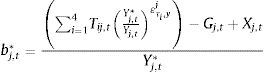

In order to analyse the cyclicality of the fiscal stance, we plot the changes in the structural primary balance against the output gap (Fig. 9). The red dots and regression line consider the real time HP gap and the blue dots and line considering the adjusted gap. Both slopes are negative, suggesting a procyclical behaviour of fiscal policy. But the slope is steeper in the case of the adjusted gap, indicating a more procyclical fiscal stance if the adjusted gap is taken as benchmark. Furthermore, the slope coefficient is non-significant in the case of the HP output gap, while it is in the case of the adjusted gap. This implies that fiscal policy is statistically neutral in the case of the HP output gap, but there is some indication of procylicality in the case of the adjusted output gap. This hints at a procyclical bias in the Latin American countries derived from the combined effect of commodity prices and capital inflows.

Fig. 9.

Procyclicality of fiscal stance.

Change in primary structural balance and real time HP output gap vs adjusted output gap.¹

This figure can be seen in colour in the electronic version.

¹The primary structural balance is constructed using the tax revenue elasticities from Alberola, Kataryniuk, Melguizo, and Orozco (2016) and including commodity revenues into each tax revenue category. For the cycle, it also considers the real time HP gap. Each point in the graph corresponds to a country – year observation of fiscal impulse and output gap.

Source: Bloomberg; Datastream; IMF, Balance of Payments; Primary Commodity Prices; UN Comtrade; UNCTAD Statistics; World Bank; national data; BIS calculations.

6

Conclusions

We have proposed and described a transparent and parsimonious method to adjust estimates of the output gap to account for the impact of financial flows and commodity prices. This is particularly relevant for Latin American countries, as their production structure and the volatility of their business cycles makes them more vulnerable to external factors, such as commodity price super-cycles and capital inflows spawned by loose monetary policies abroad.

Our findings suggest that the commodity price super-cycle has been a more relevant factor than financial inflows in explaining the output gaps. In all countries, commodity prices are significant in the multivariate filter, while capital inflows are only significant in three of the five cases. In some cases the evolution of commodity prices and capital inflows is highly correlated, but this is not a general feature of the analysis, possibly also because commodity prices incorporate a component which is tied to global demand. So, according to our analysis, real factors seem to play a larger role than purely financial factors in explaining the business cycles of Latin American countries.

In terms of the diagnosis of the state of the business cycle, our results suggest that the use of a standard HP filter to compute the output gap leads to a substantial underappreciation of imbalances building up due to buoyant commodity prices and financial inflows. This is also the case when the HP filter is computed in real time, a situation closer to that faced by policymakers. By contrast, adjusting the HP filter with commodity prices and net inflows yields results that are more robust to successive revisions, and point to a marked overheating of the economy after 2010.

In terms of policy prescriptions, it is important to take the implications with caution, first because our estimations of the adjusted output gaps cannot be taken at face value; second, because the assessment of monetary and fiscal policy is done through simple exercises. In any case, our results suggest that downplaying the role of the commodity super-cycle may have led policymakers to an excessively optimistic assessment of their economies’ potential. This in turn may have induced a procyclical bias, in particular in fiscal policy. The temptation of spending the extra revenues accruing directly from the commodity bonanza and/or the impulse on domestic demand from higher incomes is, in practice, hard to restrain. Moreover, this procyclical bias may have contributed to boost activity further beyond sustainable levels in the expansionary cycle.

The stabilisation role of monetary policy on activity is challenged by the commodity and capital inflow cycles as inflation and demand may move in different directions. Moreover, tightening monetary policy in the expansionary phase may be counterproductive, as higher rates may exacerbate capital inflows and exchange rate appreciation, thereby boosting further domestic demand and widening the imbalances. This generated a policy dilemma for Latin American countries in the booming phase of the commodity and capital flow cycle.

The limits of monetary policy under these circumstances imply that fiscal policy should lead the stabilisation effort. However, our analysis has shown that fiscal policy has been procyclical once the impact of commodity and capital cycles are taken into account.

After the reversal of the commodity super-cycle and a less buoyant financing environment, the policy space to counteract the deterioration of economic activity of the region is limited by the worsening of public accounts and inflation pressures in most countries, suggesting that the countercyclical capacity of policies is severely constrained, also in this downward phase of the cycle.

All in all, the paper suggests that improving the assessment the output gaps by taking into account the commodity cycle could help policies to stabilise more effectively activity around the potential output, in particular through facilitating the implementation of more countercyclical fiscal policies.

Conflict of interests

The authors declare that they have no conflict of interest.