Optimal v. simple financial policy rules in a production economy with “liability dollarization”

Abstract

We evaluate the effectiveness of financial policy rules in a small open economy with production, liability dollarization and “unconventional shocks” (global liquidity shifts and news about future fundamentals). Tradable and nontradable final goods are produced with tradable inputs. Debt is denominated in units of tradables and cannot exceed a fraction of the market value of total income. Optimal policy has a macroprudential or ex-ante component (a debt tax levied at date t only when the credit constraint may bind at t + 1), and ex-post components (sectoral production taxes/subsidies used when the constraint binds). The optimal policy reduces sharply the frequency and severity of financial crises but is also very complex. Simple policies are less effective and can be welfare reducing.

Resumen

Evaluamos la efectividad de las reglas de política financiera en una pequeña economía abierta con producción, dolarización de pasivos y “choques no convencionales” (cambios en la liquidez global y novedades acerca de los fundamentales futuros). Los bienes finales transables y no transables se producen con insumos transables. La deuda se denomina en unidades de bienes transables, no pudiendo exceder una fracción del valor de mercado de los ingresos totales. La política óptima tiene un componente macro-prudencial o ex-ante (un impuesto a la deuda aplicado en el periodo t solo cuando la restricción de crédito puede activarse en t+1), y componentes ex-post (impuestos/subsidios a la producción sectorial usado cuando la restricción se activa). La política óptima reduce bruscamente la frecuencia y severidad de las crisis financieras, aunque también es compleja. Las políticas simples son menos efectivas, y pueden reducir el bienestar.

1

Introduction

Recent quantitative studies show that optimal financial policy, defined as policy that implements the allocations that solve a constrained-efficient planner's problem facing a credit constraint, can be very effective at reducing the magnitude and frequency of financial crises.¹ On the other hand, these studies also show that the optimal policy has a complex state-contingent structure, which raises doubts about its feasibility and suggests that simpler policy rules should be favored. A conjecture implicit in this reasoning is that simple rules are at worse harmless and at best a good approximation to the optimal policy. The findings of recent studies suggest, however, that this conjecture is incorrect. Bianchi and Mendoza (2017) showed that simple policies can be welfare-reducing, because they may not match well the prudential characteristics of the optimal policy, which tightens credit-market access in periods of expansion, with a magnitude that varies with the likelihood and severity of future credit crises, and eases credit conditions in the opposite situations. Hence, there is a delicate tradeoff in financial policy design: The optimal policy is too complex to be feasible operationally, but arbitrarily chosen policy rules can be harmful.

This issue is of major policy relevance, because it highlights the importance of the specific rules setting the conditions that trigger the use of financial stability policy instruments and their evolution over time, and yet there is little guidance about the quantitative features that these rules should have. For instance, the Basel III Countercyclical Capital Buffer (CCyB) has the same macroprudential aim of the optimal financial policy described above (i.e. tightening credit in periods of expansion), but it did not define specific rules for when the CCyB is triggered and for how it moves over time. Instead, it left these key features of the CCyB to be determined by BIS member countries using their own judgment. In particular, Basel III indicates that: “each jurisdiction will be required to monitor credit growth and make assessments of whether such growth is excessive and is leading to the build up of system-wide risk. Based on this assessment they will need to use their judgment, following the guidance set out in this document, to determine whether a countercyclical buffer requirement should be imposed. They will also need to apply judgment to determine whether the buffer should increase or decrease over time (within the range of zero to 2.5% of risk weighted assets) depending on whether they see system-wide risks increasing or decreasing. Finally they should be prepared to remove the requirement on a timely basis if the system-wide risk crystallizes.”²

In this paper, we compare optimal and simple financial policy rules using a quantitative Fisherian model of financial crises similar to a model widely used in the literature, in which a small open economy faces an endogenously-binding collateral constraint and displays “liability dollarization.”³ In particular, debt is denominated in units of tradable goods and cannot exceed a fraction of the income from tradables and nontradables. Models in this Fisherian class feature an endogenous financial amplification mechanism that produce infrequent financial crises with realistic features.

As the literature has shown, the market failure that justifies policy intervention in these models is a pecuniary externality that exists because goods used as collateral are valued at market prices. The social marginal cost of borrowing exceeds the private marginal cost because private agents do not internalize the negative effects of their individual borrowing decisions made in normal times on collateral prices in crisis times. When a crisis hits, the collateral constraint binds inducing agents to fire-sale goods, which in turn causes a collapse in the relative price of nontradable goods, which tightens the constraint further and induces larger declines in relative prices triggering Fisher's classic debt-deflation mechanism.

The model we propose is based on the one developed by Bianchi et al. (2016), who introduced noisy news about future economic fundamentals and regime shifts in global liquidity to the workhorse model of macroprudential policy with liability dollarization. We modify this setup by introducing production of tradable and nontradable goods using intermediate goods. This has two important implications. First, it introduces a mechanism by which the collateral constraint causes a drop in output in crisis episodes, because the collapse of the relative price of nontradables causes a collapse in demand for inputs in production of nontradables. Second, as a result of the supply-side effects of the collateral constraint, it provides additional vehicles for policy intervention by introducing inefficiencies in sectoral production and factor allocations during crises.

We characterize optimal policy in the model, showing how the constrained-efficient social planner has incentives to implement both macroprudential and ex-post financial policies. The former reflects the standard pecuniary externality from the existing literature: the optimal policy seeks to increase the cost of borrowing when the collateral constraint is not binding in the current period but can bind with positive probability next period, so as to induce private agents to face the social marginal cost of borrowing in periods of expansion. The ex-post financial policies result from the fact that the effects of the crisis can be mitigated by reallocating resources from production of nontradables to production of tradables in order to prop up the value of collateral and enhance borrowing capacity. Both macroprudential and ex-post financial policies are decentralized as optimal taxes. The macroprudential policy takes the form of a debt tax, and the crisis-management policies take the form of sectoral production taxes and subsidies.⁴ Following Bianchi et al. (2016), we also characterize the effects of news about fundamentals and global liquidity shifts on the optimal policies.

The model is calibrated to data from Colombia and solved to illustrate the model's crisis dynamics in the absence of policy intervention, the effectiveness of the optimal policy, and the comparison with simple policy rules. The optimal policy reduces the magnitude and severity of financial crises significantly. In contrast, simple policies are much less effective and can be welfare reducing. In particular, time-invariant taxes set to the average values under the optimal policy yield an outcome with lower social welfare than the competitive equilibrium without policy intervention. The time-invariant taxes that yield the largest welfare gain can only produce a gain about half as large as under the optimal policy, have crises in which consumption and the real exchange rate drop nearly four times more, and have crises with a frequency of 1.1% (v. nearly zero with the optimal policy).

The rest of the paper is organized as follows. Section 2 describes the decentralized equilibrium of the model without policy intervention. Section 3 examines the problem solved by the financial regulator, characterizes the optimal policy, and shows how the allocations of the social planner can be decentralized using taxes on debt and producers’ input purchases. Section 4 examines the quantitative predictions of the model. Section 5 provides conclusions.

2

Model

Our analysis is based on a two-sector model with liability dollarization that has been widely studied in the literature on emerging markets sudden stops and on optimal macroprudential policy (e.g. Mendoza, 2002; Bianchi, 2011). In particular, we extend the variant of this model proposed by Bianchi et al. (2016) that features noisy news about future fundamentals and global liquidity regime-switches by introducing production of tradable and nontradable goods. Durdu et al. (2009) proposed a similar setup but with production only in the nontradables sector, keeping tradable goods as an endowment, and they abstracted from studying the normative implications of the model.

2.1

Households and firms

The model represents a small open economy in which a representative household consumes tradable and nontradable goods, denoted c^T and c^N respectively, and representative firms produce tradable and nontradable goods using intermediate goods, denoted m^T and m^N in each industry respectively. The household collects the profits of the firms (π^T and π^N) and has access to a world credit market of non-state-contingent bonds (b) denominated in units of tradable goods. Goods and factor markets are competitive and the prices of traded goods (including both consumption and intermediate goods) and bonds are taken as given from world markets. The credit market is imperfect, because borrowing is limited to fraction of the agent's income in units of tradable goods.

The preferences of the representative agent are given by a standard intertemporal utility function with constant relative risk aversion (CRRA) defined over a composite good c_t:

E(·) is the expectation operator, β is the discount factor, and γ is the coefficient of relative risk aversion. The composite good is modeled as a CES agregator:

The elasticity of substitution between ctT and ctN is given by which 1/(η + 1). This is an important parameter because, as we show later, is one of the main determinants of the collapse of the real exchange rate in periods of financial crises, which in turn is the main driver of crisis dynamics in the model.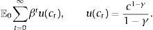

Choosing the world-determined price of tradable goods as the numeraire, the agent's budget constraint is:

The left-hand-side of this expression shows the uses of the agent's income: purchases or sales of bonds b_t+1 at the world-price q_t (the inverse of which is the world real interest rate R_t), plus total expenditures in consumption of tradable and nontradable goods in units of tradables, denoting the relative price of nontradables as ptN. A^T and A^N are constant levels of autonomous expenditures that represent investment and government expenditures, which are introduced so that the model can be calibrated to actual consumption–GDP ratios. The right-hand-side of the budget constraint shows the sources of the agent's income: Income from maturing bond holdings b_t (or repayment of debt if b_t < 0), and profits from production of tradables and nontradables.

Borrowing requires collateral and only a fraction of the agent's income is pledgeable as collateral. As a result, the representative agent cannot borrow more than a fraction κ of total income in units of tradables (i.e. a fraction of total profits):

This constraint can be interpreted as the result of enforcement or institutional frictions by which lenders are only able to harness a fraction κ of a defaulting borrower's income, or borrowers can only pledge a fraction κ of their income as collateral. It can also be viewed as resulting from conventional practices in credit markets, such as the loan-to-income ratios used to limit household credit or in the construction of credit scores.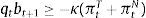

As noted earlier, the model's approach to model two sectors, tradables and nontradables, with debt denominated in units of tradables, aims to capture the so-called liability dollarization phenomenon typical of emerging economies: Foreign liabilities denominated in hard currencies, which represent tradable goods, backed up by the income generated in both tradables and nontradables sectors.

The representative agent chooses optimally the sequences {ctT,ctN,bt+1}t≥0 to maximize (1) subject to (3) and (4), taking b₀ and ptN,πtT,πtNt≥0 as given. This maximization problem yields the following first-order conditions:

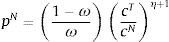
where λ_t and μ_t are the Lagrange multipliers on the budget constraint and credit constraint respectively, and u_T is the marginal utility of consumption of tradables.

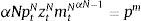
The representative firms in both industries use inputs, purchased at a world-price p^m, to produce. They operate Neoclassical production functions ztimtiαi, for i = T, N, facing sectoral TFP shocks (zti for i = T, N) that follow a Markov process to be specified later. We abstract from modeling capital and labor for simplicity. They can be assumed to enter the production technologies in fixed unit supply. Profits are given by:

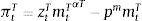
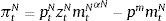
The demand for inputs is chosen so as to maximize profits in each sector. This yields standard optimality conditions equating the value of the marginal product of inputs with the relative price in each industry:

It is critical that the relative price of nontradables determines the value of the marginal product of inputs in the production of nontradables, because financial crises in the model produce an endogenous drop in output of nontradables, which is induced by a drop in demand for inputs due to a collapse in the relative price of nontradables. Note also that fluctuations in production of tradable goods and in the demand for inputs from that sector, are solely driven by the industry's TFP shock, and hence are unaffected by a financial crisis.

2.2

Competitive equilibrium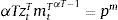

The competitive equilibrium is given by sequences of allocations {ctT,ctN,mtT,mtN,bt+1}t≥0, profits πtT,πtNt≥0 and prices ptNt≥0 such that: (a) the representative agent maximizes utility subject to the budget and collateral constraints taking prices and profits as given, (b) the representative firms maximize profits taking prices as given, and (c) the market-clearing condition of the market of nontradables (ctN+AN=ztNmtNαN) and the resource constraint of tradables (ctT+AT=ztTmtTαT−pm(mtT+mtN)−qtbt+1+bt) hold.

Notice that the cost of inputs used in both industries enters in the resource constraint of tradables. Algebraically, this follows from noticing that equilibrium profits are πtT=(1−αT)ztTmtTαT and πtN=(1−αN)ptNztNmtNαN in the tradables and nontradables sector respectively, and then using these results to replace profits in the household's budget constraint, and applying the nontradables market-clearing condition. Intuitively, this makes sense because inputs are assumed to be tradable goods, regardless of whether they are used to produce tradables or nontradables. Hence, the economy's balance of trade is given by ytT−pm(mtT+mtN)−ctT−AT. Note also that gross production and GDP in units of tradable consumer goods are given by ytG=ytT+ptNytN and GDPt=ytG−pm(mtT+mtN) respectively.

2.3

News and global liquidity regimes

We use the same formulation of news about fundamentals and global liquidity regime switches as in Bianchi et al. (2016). They followed the work of Durdu et al. (2013) to model news as noisy signals received at date t about the value that zt+1T may take. Notice that in this setup news about future TFP of the tradables sector or about future world-determined relative prices of exportable goods in terms of a world basket of tradables (i.e. the small open economy's terms of trade) are equivalent. This is useful because it implies that we can think of the noisy news as related to future real commodity prices, which are a key source of volatility for many emerging economies.

The probability of a news signal conditional on a date−t + 1 tradables TFP realization is given by the following condition:

where s_t is the signal at date t, Z is the number of possible realizations of zt+1T, and θ is the signal precision parameter. When θ = 1/Z, the signals are completely uninformative, because p(st=i|zt+1T=l) simply assigns a uniform probability of 1/Z to all values the signal can take at t, regardless of the value of zt+1T. In this case, news do not add any information useful to alter the expectations about zt+1T that are formed using the probabilistic process of z^T alone. Conversely, θ = 1 implies that the signals have perfect precision. The agent can perfectly anticipate the value of zt+1T (e.g. zt+1T=l is expected to occur for sure when the signal s_t = l is observed). Perfect precision does not, however, remove tradables TFP uncertainty completely, because future signals themselves are stochastic, so uncertainty about TFP for dates t + 2 and beyond remains, although now expectations of future TFP are based only on expectations of future signals.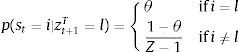

Following Durdu et al. (2013), we can use Bayes's Theorem to derive the conditional forecast probability of tradables TFP at date t + 1 conditional on a particular date−t pair (ztT,st), and then form Markov transition probabilities for the joint evolution of z^T and s:

These probabilities are used by the representative agent to form expectations when solving the expected utility maximization problem. Notice that Π(·) combines the information provided by the date−t signal and TFP realization about the likelihood of a particular date−t + 1 TFP realization being associated with a particular new signal. The representative agents know that signals themselves are stochastic, and hence forms rational expectations about their future evolution.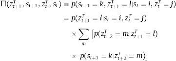

Fluctuations in global liquidity are modeled as a standard two-point, regime-switching Markov process that can drive either fluctuations in the world real interest rate or in the fraction of income that can be pledged in credit markets. The regime realizations are x^h (low liquidity) and x^l (high liquidity) with x^h > x^l for x = R, κ. Continuation transition probabilities are denoted F_hh ≡ p(x_t+1 = x^h ∣ x_t = x^h) and F_ll ≡ p(x_t+1 = x^l ∣ x_t = x^l), and switching probabilities are F_hl = 1 − F_hh and F_lh = 1 − F_ll. The long-run probabilities of each regime are Π^h = F_lh/(F_lh + F_hl) and Π^l = F_hl/(F_lh + F_hl) respectively, and the mean durations are 1/F_hl and 1/F_lh.

3

Optimal financial policies

Following Bianchi (2011), we study optimal financial policy by first characterizing the solution to a constrained planner's (or financial regulator's) problem, in which the regulator chooses directly the economy's bond holdings (i.e. debt) facing the same credit constraint as private agents, but lets all other markets operate competitively.

The regulator's optimal policy problem can be formulated as a recursive dynamic programming problem, following the standard convention of denoting with a prime variables dated t + 1:

subject to

This Bellman equation has a single endogenous state variable, current bond holdings, b, and four exogenous shocks that are included in the vector of exogenous states: e = (z^T, z^N, s, q) .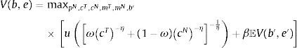

The constraints in the regulator's optimal policy problem include: the resource constraint for tradables (16), the market-clearing condition for nontradables (17), the credit constraint with profits as determined in competitive markets (18), plus an implementability constraint that requires that the equilibrium price of nontradables matches the representative agent's marginal rate of substitution in consumption of tradables and nontradables (19) Deriving the first-order conditions of the regulator's problem, simplifying them, and expressing them in sequential form yields:

In these expressions, λ_t and μ_t are the Lagrange multipliers on the resource constraint and credit constraint respectively, and ψt≡[(1+η)((ptN[(1−αN)ztNmtNαN))/ctT)].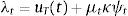

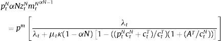
The term ψ_t in the first optimality condition measures how the regulator's choice of b_t+1 affects borrowing capacity via its effect on tradables consumption and the equilibrium price of nontradables (i.e. by affecting the value of collateral). It follows then that the term μ_tκψ_t shows that, when the credit constraint binds, the social marginal benefit from consumption of tradable includes not only the marginal utility of tradables consumption, but also the gains resulting from how changes in tradables consumption help relax the credit constraint. Note also that the magnitude of ψ_t falls with the elasticity of substitution in consumption of tradables and nontradables, because the price of nontradables falls less during a crisis the higher this elasticity, and rises with the ratio of profits from the nontradables sector to consumption of tradables.

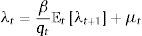
Optimal financial policy in this setup includes macroprudential or ex-ante policy, defined as policy used when the credit constraint is not binding at date t but can bind with some probability at t + 1, and ex-post financial policy, defined as policy that is active when the constraint binds at date t. In particular, the aim of the macroprudential policy is to affect credit allocations in normal times because of what those allocations can cause during crisis times. Hence, this type of policy is active when μ_t = 0 but E_t[μ_t+1] > 0. In this scenario, the regulator's Euler equation (Eq. (21)) takes this form:

Comparing this condition with the household's Euler equation for bonds shows that this model features the familiar wedge between the private and social marginal cost of borrowing from the literature on macroprudential policy, which is given by the term μ_t+1κψ_t+1. In particular, when the credit constraint is expected to bind, the regulator faces a strictly higher marginal cost of borrowing than the representative agent. This is a pecuniary externality, because it results from the fact that the regulator evaluates borrowing choices at t taking into account that the credit constraint could bind at t + 1, and if it does the Fisherian debt-deflation mechanism will cause a collapse of the relative price of nontradables (i.e. a collapse of the real exchange rate) that will shrink borrowing capacity. The representative agent takes prices as given, and thus does not internalize these effects.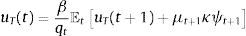

The terms in square brackets in the right-hand-side of the third and fourth optimality conditions (Eqs. (22) and (23)) capture the regulator's incentives to use financial policy ex-post, when the credit constraint binds. In particular, when μ_t > 0, the regulator finds it optimal to introduce wedges between the value of the marginal product of inputs and their marginal cost in each sector, which indicates that the sectoral social marginal costs of inputs differ from the private marginal cost p^m.

Consider first the wedge in the regulator's optimality condition for production of nontradables. This wedge captures the effects of changes in inputs allocated to production of nontradables on borrowing capacity induced via changes in the output and price of nontradables.⁵ Borrowing capacity is affected by three effects: First, an increase in demand for inputs, which are tradable goods, reduces resources available for tradables consumption, contributing to lower the nontradables price. Second, the increased production of nontradables obtained with the increase in inputs also lowers the price of nontradables because of the higher supply of these goods. Third, the additional profits generated by the increase in production increase pledgeable resources. The first two effects reduce borrowing capacity while the third increases it. The first two effects are also pecuniary externalities, because they capture price effects of production decisions that are not internalized by private nontradables producers, and the third effect is a non-pecuniary externality that captures the effects of these producers’ decisions on the representative agent's access to world debt markets, which are not internalized by firms.

The wedge in the regulator's optimality condition for production of tradables has a similar intuition: It captures the effects of changes in inputs allocated to production of tradables on borrowing capacity induced via changes in the output and price of nontradables. Effects analogous to the first and third effects referred to above are again present (i.e. again higher demand for inputs reduces tradables consumption and makes the price of nontradables and borrowing capacity drop, and again higher profits enhance borrowing capacity). The second effect, however, does not operate because production of tradables does not alter directly the supply of nontradables.

It is critical to note that the social marginal cost of inputs in the production of nontradables is higher than the private marginal cost (i.e. the wedge in Eq. (22) is less than 1), while the opposite is true in the tradables sector (i.e. the wedge in Eq. (23) is higher than 1). This is because the second term in the denominator of (22) is unambiguously negative while the second term in the denominator of (23) is unambiguously positive. Hence, although effects of the regulator's optimal plans affecting borrowing capacity in opposite directions are at work in both sectors, as explained above, the isoelastic production and utility functions we are using imply that the effects reducing borrowing capacity dominate in the nontradables sector, and the effects increasing borrowing capacity dominate in the tradables sector.

News about future TFP in the tradables sector (e.g. about future terms of trade or commodity prices) and regime-switches in global liquidity have important effects on the externalities driving both macroprudential and ex-post policies. As Bianchi et al. (2016) explained, “good news” at t about productivity in the tradables sector at t + 1 lead to higher consumption, and since the resulting gain in income has not been realized yet, this leads to an increase in borrowing which makes the economy more vulnerable to hitting the credit constraint. On the other hand, by increasing expected future income, good news also increase on expectation the future borrowing capacity and at the same time reduce future borrowing needs. Similarly, a shift into a regime with high global liquidity leads the economy to take on more debt (e.g. a switch to a lower interest rate makes borrowing cheaper). A sudden shift into a low global liquidity regime can lead to a decline in consumption, which in turn makes the credit constraint tighter and leads to a sharp reduction in both production and capital flows, and a drop in the real exchange rate (i.e. the relative price of nontradables).

The constrained-efficient allocations and prices that solve the planner's problem can be decentralized as a competitive equilibrium using various policy instruments, including taxes on debt, debt-to-income ratios, capital requirements or reserve requirements (see Bianchi, 2011; Stein, 2012). Since the market failures are in the form of externalities, the natural instruments to consider are standard taxes on the cost of the good associated with each externality. In particular, the regulator can implement the optimal allocations by taxing debt, taxing input purchases in the nontradables sector, and subsidizing input purchases in the tradables sector.

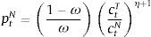
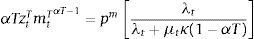
With a debt tax, the cost of purchasing bonds in the budget constraint becomes [q_t/(1 + τ_t)]b_t+1. We assume also that the revenue of the tax is rebated to the household as a lump-sum transfer to neutralize income effects from this tax. The optimal macroprudential tax is then the value of τ_t that equates the Euler equations of bonds of the regulator and the decentralized equilibrium with the tax. Hence, the tax induces private agents to face the social marginal cost of borrowing in the states in which this cost differs from the private cost in the absence of macroprudential policy. When μ_t = 0, the optimal macro-prudential tax is:

Notice that the numerator of this tax is equal to the expected value of the pecuniary externality.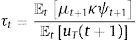

With a tax τtN on input costs in the nontradables industry, the total cost of inputs in that sector becomes pm(1+τtN)mtN. Similarly, with a subsidy s^T on input costs in the tradables industry, the total cost of inputs in that sector becomes pm(1−stT)mtT. The optimal gross tax and subsidy are those such that (1+τtN) and (1−stT) match the wedges in the square-bracket terms in the right-hand-sides of Eqs. (22) and (23) respectively. Hence the optimal tax and subsidy are:

Since the social marginal costs of inputs differ from the private marginal cost only when the constraint binds at date t, both the tax and the subsidy are zero if the constraint is not binding. When the constraint binds, the government taxes production of nontradables and stimulates the production of tradables (both the tax and subsidy rates are strictly positive when μ_t > 0). Notice also that profits are still given by the same expressions as before, because the optimality conditions for the demand for inputs with the tax and subsidy still imply that profits are πtN=(1−αN)ztNmtNαN (πtT=(1−αT)ztTmtTαT). Hence, in order to neutralize the budgetary effects of these production taxes and subsidies at equilibrium, we can assume that households are levied lump-sum taxes to pay for subsidies and lump-sum transfers to rebate tax revenues.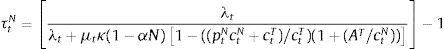

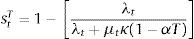
It is worth noting that, according to the above two conditions setting the optimal production taxes and subsidies, we should expect taxes on nontradables to be much larger in absolute value than subsidies on tradables. The expressions for the two are similar, and in addition in our calibration αT > αN, which tends to make the subsidy on tradables larger than the tax on nontradables. But the key difference in the two expressions is the term in square brackets in the denominator of the nontradables tax, which in turn captures the effect missing from the wedge in the optimal allocation of inputs for tradables production relative to that pertaining to nontradables production mentioned earlier: Production of tradables does not alter directly the supply of nontradables, while production of nontradables does, and this in turn affects the value of collateral (p^N) and thus borrowing capacity. This effect is larger the larger is nontradables consumption relative to tradables consumption.

With the three policy instruments and lump-sum taxes and transfers in place, the budget constraint of the household becomes:

The government sets Trt=−qtbt+1(τ/1+τ)+τtNmtN−stTmtT, which is a lump-sum transfer if positive or tax if negative. Substituting profits from the producers’ optimal plans, using the nontradables market-clearing condition, and the government's total transfers, we recover again the resource constraint for tradables of both the decentralized equilibrium and the planner's problem.

It is worth noting that this setup also preserves the property that the debt tax is inessential when the collateral constraint binds, as in the setup of Bianchi et al. (2016). Any value of τ_t consistent with the collateral constraint being binding in the competitive equilibrium with taxes (i.e. any τ_t such that U_T(t) > (β/q_t)(1 + τ_t)E_t[U_T(t + 1)]) can support the planner's allocations and prices. With the tax and subsidy on input purchases by producers of nontradables and tradables set to their corresponding optimal values when the constraint binds, the consumption, input and debt allocations are determined without the consumption Euler equation, and therefore without the debt tax. For simplicity, we set the debt tax to zero in these situations, after verifying that it is in the range of inessential debt taxes.

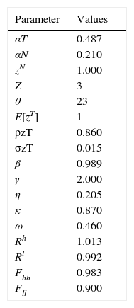
4

Quantitative analysis

4.1

Calibration

The parameterization follows the one constructed by Bianchi et al. (2016), but here we use data for Colombia and use a quarterly frequency. The main difference is in that, since we have added production with intermediate goods into the model, we need to calibrate the sectoral shares of intermediate goods in the production functions of tradables and nontradables and the sectoral TFP shocks. The parameter values used to calibrate the model are shown in Table 1.

Table 1.

Baseline calibration.

Parameter	Values
αT	0.487
αN	0.210
z^N	1.000
Z	3
θ	23
E[z^T]	1
ρzT	0.860
σzT	0.015
β	0.989
γ	2.000
η	0.205
κ	0.870
ω	0.460
R^h	1.013
R^l	0.992
Fhh	0.983
Fll	0.900

As in Bianchi et al. (2016), we set the coefficient of relative risk aversion to γ = 2, which is a standard value. We also follow their calibration in setting η = 0.205. The value of this parameter is important because, as we explained earlier, the elasticity of substitution in consumption of tradables and nontradables (1/(1 + η)) is a key determinant of the response of the price of nontradables to changes in sectoral consumption allocations, and hence of the size of the pecuniary externality and the collapse in the nontradables price when a crisis hits.

The factor shares of intermediate goods in production of tradables and nontradables are set according to information from the Colombian input–output matrix. Since we are abstracting from nontradable inputs, we re-define gross production in each sector as the sum of value added plus tradable inputs, with the breakdown between tradable and nontradable sectors constructed by defining the former as including those sectors for which total trade (exports plus imports) exceeds 10% of gross production. The value of αT is then set equal to the ratio of tradable inputs used in all tradable sectors to the combined gross output of all tradable sectors, and similarly, the value of αN is set equal to the ratio of tradable inputs used in the nontradables sector to the combined value added of all nontradable sectors. This results in factor shares of 49 and 21% in the tradables and nontradables sector respectively. Notice from expressions (26) and (27) that both the tax on nontradables and the subsidy on tradables are higher when their corresponding factor share is lower, with a factor of proportionality that depends on μ_tκ.

The joint Markov process of the tradables productivity and news signals is set as follows. First, we set ρzT=0.860 and σzT=0.015 so as to match the first-order autocorrelation and standard deviation of the HP-filtered cyclical component of GDP from Colombian data. Second, we use the Tauchen–Hussey quadrature algorithm to construct a Markov process with three realizations of tradables TFP shocks (Z = 3). Third, to set the value of θ, recall that we are assuming that the signals also have three realizations. Hence, θ = 1/3 makes news completely uninformative and θ = 1 makes news a perfect predictor of yt+1T as of date t. Thus, following again Bianchi et al. (2016), we set θ to the mid point between these two extremes so that θ = 2/3. For simplicity, we also assume that the signal realizations and the vector of realizations of z^T are identical, and we abstract from TFP shocks in the nontradables sector.

Fig. 1.

Global liquidity regimes.

The regime-switching process of the world interest rate also matches the one used by Bianchi et al. They constructed it so as to capture the global liquidity phases identified in the studies by Calvo et al. (1996) and Shin (2013), using data on the ex-post net real interest rate on 90-day U.S. treasury bills from the first quarter of 1955 to the third quarter of 2014. Calvo et al. identified in data for the 1988–1994 period a surge in capital inflows to emerging markets that coincided with a trough of −1% in the net U.S. real interest rate in the second half of 1993. Shin found two global liquidity phases, one in the first half of the 2000s with a real interest rate through of around −5.5% in early 2004, and another one in the aftermath of the 2008 global financial crisis, with the net real interest rate hovering around −3% since 2009. Taking the average over the troughs in the Calvo et al. sample and in the first of Shin's global liquidity phases, we set a −0.82% real interest rate for the high liquidity regime, which in gross terms implies R^l = 0.9918. Given this, and the transition probabilities across regimes calibrated below, we set R^h = 1.013 so that the mean interest rate of the regime-switching process matches the full-sample average in our data, which was 1%.

Constructing estimates of the duration of the global liquidity phases is difficult, because the era of financial globalization, and hence global liquidity shifts, started in the 1980s, and of the three global liquidity phases observed since then, the third is heavily influenced by the unconventional policies used after the 2008 crisis. Using data from the first two phases, it follows that the duration of R^l was 10 quarters, which thus leaves a duration of 60 quarters for R^h, starting the sample in 1980. This yields F_hh = 0.983 and F_ll = 0.9 at quarterly frequency.

The discount factor β is set to match an average net foreign asset position–GDP ratio of −0.79, which is the quarterly equivalent of the annual average for Colombia in the data of Lane and Milesi-Ferretti (2001). We set ω = 0.460 to obtain a share of tradables output over total output of 0.30 for Colombia in a deterministic version of the model with constant b. Given the calibrated value of b, ω is obtained from yT/((1−ω)/ω((yT+(R−1)b)/yN)η+1yN+yT)=0.30.⁶

Finally, we calibrate the value of κ so that, conditional on all the other calibrated parameter values, the model yields a frequency of crises of 3%, in line with estimates of the annual frequency of financial crises and sudden stops (see Mendoza, 2010). This yields a value of κ = 0.87. We target the annual frequency of crises because in the quarterly model simulation we count successive quarters of a financial crises as a single event.

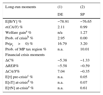
4.2

Long-run and financial crisis moments

Table 2 shows a set of the moments that characterize the decentralized equilibrium without policy intervention (DE) and the social planner's equilibrium (SP) with the optimal financial policy. The top panel shows the mean net foreign asset position–output ratio, the standard deviation of the current account–output ratio, the welfare gain of adopting the optimal policy, the probability of a financial crisis, the probability of observing a binding collateral constraint, and the probability of being in the macroprudential tax region (i.e. the probability that μ_t = 0 and E_t[μ_t+1] > 0).⁷

Table 2.

Baseline model moments.

Long-run moments	(1)	(2)
	DE	SP
E[B/Y] %	−78.91	−76.65
σ(CA/Y) %	2.11	0.99
Welfare gain^a %	n/a	1.27
Prob. of crisis^b %	2.95	0.00
Pr(μt > 0) %	16.79	3.20
Prob. of MP tax region %	n.a.	10.01
Financial crisis moments
ΔC%	−5.38	−1.33
ΔRER%	−5.58	−0.59
ΔCA/Y%	7.04	−0.35
E[τ] pre-crisis^c %	n.a.	0.05
E[sT] at-crisis^d %	n.a.	0.07
E[τN] at-crisis^e %	n.a.	0.61

a

Welfare gains are computed as compensating variations in consumption constant across dates and states that equate welfare in the DE and SP. The welfare gain W at state (b, z) is given by (1 + W(b, z))^1−σV^DE(b, z) = V^SP(b, z). The long-run average is computed using the ergodic distribution of the DE.

b

A financial crisis is defined as a period in which the constraint binds and the current account (CA/Y) raises by more than two standard deviations in the ergodic distribution of the decentralized economy, which implies a reversal in (CA/Y) larger than 4.2%.

c

Average τ in the period before financial crises.

d

Average s^T in starting period of financial crises.

e

Average τ^N in the starting period of financial crises.

The mean debt ratios are similar in the two scenarios. In the DE baseline calibration, we set β = 0.989 to match the average quarterly NFA–GDP ratio in the data for Colombia. The mean debt ratio of the planner is slightly smaller (76.7%), because of the reduced incentive to borrow once the pecuniary externality is removed. In contrast, the variability of the current account in DE is roughly twice as large as in SP. Thus, the two economies support similar long-run debt positions, but the optimal financial policy halves the volatility of capital flows. This finding is in line with Bianchi (2011), who showed that optimal macroprudential policy achieves a reduction in volatility despite small changes in average debt ratios.

The optimal policy also reduces the probability of crises from 2.95% in DE to 0 in SP, and the probability that the constraint binds falls from 16.8% to 3.2%. Note that in the DE the frequency with which the constraint binds (16.8%) is 5.7 times the frequency with which financial crises occur, hence there are several periods in which the constraint binds but there is no crisis (i.e. the correction in the debt position is not enough to trigger a sufficiently large current account reversal). The frequency with which the macroprudential tax is active in the SP scenario is about 10%, while the frequency with which the production taxes and subsidies are used is only 3.2% since these taxes are used only when the collateral constraint binds for the planner. These frequency results, however, are not informative about the size of the taxes and subsidies, they only measure the likelihood of observing them.

The optimal policy increases social welfare by a sizable amount, equivalent to a permanent increase of roughly 1.3% in consumption. This is interesting because typically welfare gains of smoothing fluctuations are negligible in standard business cycle models with CRRA preferences. In this model, the gains are larger because of both the significant reduction in long-run volatility and the removal of infrequent but dramatic crisis events, in which quarterly consumption drops significantly, as we show next.

The bottom panel of Table 2 shows moments that summarize the main features of financial crises in both the DE and SP solutions. First we report three statistics about the average magnitude of crises: the drops in aggregate consumption (ΔC) and the real exchange rate (ΔRER), and the reversal in the current account–output ratio (ΔCA/Y). For the DE, these statistics are averages of the impact effects that occur when a financial crisis hits, computed with the corresponding economy's long-run distribution of the state variables (b, z) conditional on the economy being in a financial crisis state. For the SP, we report averages of the responses of the variables under identical sequences of exogenous shocks as in the DE using the SP's long run distribution. The Table also shows the average macroprudential tax before a crisis occurs (Eτ pre-crisis), the subsidy on input costs of the tradables sector (EsT), and the tax on input costs of the nontradables sector (EτN).

The results in the DE column show that financial crises in this model result in large declines in consumption and the real exchange rate, and large current-account reversals. The much smaller fluctuations in the SP column show that the optimal financial policy reduces significantly the severity of crises.

In terms of the policy instruments, the size of the taxes and subsidies is small: On average over the three years before a crisis, the macroprudential debt tax is 0.05%, while the averages across crises periods for the subsidy on tradables producers and the tax on nontradables producers are 0.07 and 0.61% respectively (with the latter nearly 9 times bigger than the former). Hence, in this model the optimal financial policy is quite effective at reducing the frequency and severity of financial crises with relatively small taxes and subsidies.

The effects of the pecuniary externality on borrowing choices, particularly the incentive to over-borrow in the DE, and the effectiveness of the macroprudential policy at containing these effects are both illustrated in the long-run distributions of bond holdings shown in Fig. 2. Note also that the twin-peaked nature of these distributions results from the twin-peaked distribution of interest-rate shocks characteristic of their two-point, regime-switching specification.

Fig. 2.

Ergodic distributions of bond holdings.

4.3

Crisis dynamics

We study next macroeconomic dynamics around crisis events. Fig. 3 plots event-analysis windows for the price of nontradables, the debt choice, aggregate consumption and the current account–GDP ratio that highlight these dynamics. The windows show deviations from long-run averages spanning seven quarters, centered on the quarter a crisis occurs, with the DE shown in continuous, red curves and the SP in dashed, blue curves.⁸ The movements observed when financial crises hit in the DE emerge as sharp, non-linear drops in the nontradables prices, debt and consumption, and a sharp current account reversal (i.e. a Sudden Stop), relative to the much smoother pre-crisis patterns.⁹ Recoveries after crisis are relatively slow in the DE, with prices, debt and consumption still sharply below their long-run means three quarters after the crisis hits. The effectiveness of the optimal financial policy at reducing the severity of crises is evident in the much smoother dynamics of the SP economy.

Fig. 3.

Baseline DE v. SP around crises. (For interpretation of the references to color in text, the reader is referred to the web version of the article.)

Fig. 4 shows the composition of the shocks at work in the model in the seven periods covered in the event windows, by plotting the fraction of realizations of each shock that were observed each quarter. The top panel is for news signals, the mid panel for interest rate regimes, and the bottom panel for tradables TFP shocks. As one would expect, financial crises are periods that largely coincide with high real interest rates and low productivity/income realizations. On the other hand, less than 55% of financial crises coincide with bad news (i.e. bad news at t = 0 in the top panel of the Figure). The pre-crisis phase is characterized also by mainly high interest rates, and by average or bad TFP shocks. In contrast, and in line with the intuition for the mechanism relating news to financial crises described earlier, in the pre-crisis phase there is a non-trivial fraction of observations of good and average news. Hence, several crisis episodes are preceded by good and average TFP news in the periods leading up to the crisis, followed by actual low TFP realizations when the crisis hits.

Fig. 4.

Exogenous shocks around crises events.

4.4

Complexity of the optimal policy

The results discussed up to this point show that the optimal financial policy is very effective, in terms of reducing the frequency and severity of financial crises and increasing social welfare. We show next that, despite these positive results, the optimal policy is also very complex. Implementing the optimal debt and production taxes is challenging because they require precise knowledge of the state of the economy at each point in time. In particular, the optimal macroprudential debt tax requires knowing the probability that a crisis may hit one period ahead conditional on financial and macroeconomic conditions in the current period. But even if precise information is available, the results we report below show that the optimal policy has significant variation over time and across states of nature.

Fig. 5 shows the evolution of the optimal policy instruments in the regulated decentralized economy around financial crises events. The top-left plot shows the probability of the leverage constraint being binding. The other three plots show the evolution of the optimal macroprudential debt tax, the nontradables input tax and the tradables input subsidy. For these three, the plots show unconditional averages for each period of the event windows, and in addition for the input tax and subsides we show averages conditional on the leverage constraint being binding (since when the constraint does not bind both are zero), and for the debt tax we show the average conditional on the constraint not being binding (since when the constraint binds the debt tax is zero).

Fig. 5.

Policy instruments around crisis events.

The plot of the macroprudential debt tax shows the pro-cyclical nature of this policy. Conditional on credit not being constrained, the macroprudential debt tax rises from about 0.03 to a just above 0.08% in the quarters before the crisis, and falls to near 0.04% in the post-crisis phase. Thus, while debt taxes are low on average, they still display significant variability over time. In addition, debt taxes are very active around crisis times. Recall from Table 2 that the debt tax is active 10% of the time in the long run, but the fact that the unconditional and conditional-on-unconstrained-credit averages in the event window are very similar suggests that this policy is active most of the time in the periods covered by the window. The probability with which the debt tax is being used each period cannot be inferred unambiguously from the gap between the two averages, because the constraint not being binding at t is necessary but not sufficient for the debt tax to be used. This requires in addition that the constraint is expected to bind at t + 1 at least in some states of nature.

The evolution of input taxes and subsidies around crises is countercyclical, and the averages conditional on the constraint being binding are much higher than the unconditional averages. This occurs because these two instruments are zero when the constraint does not bind, and the probability of the constraint being binding for the planner is generally low. Focusing on averages when the constraint binds (i.e. when these instruments are used), the tax on inputs for the nontradables sector falls from about 2.8% to 2% in the pre-crisis phase, and then rises gradually to about 2.5% in the post-crisis phase. The subsidy on inputs for the tradables sector falls from 0.33% to 0.24%, and then rises back to about 0.3%. Thus, while less volatile in terms of variance than the debt tax, these two instruments also fluctuate markedly around crisis times. Moreover, in terms of rates at which the three instruments are set, the tax on nontradables has a much higher average hovering around 2.5% (conditional on the constraint being binding). This is because of the direct effect of the nontradables tax on the supply of nontradables, and hence on its relative price, discussed earlier.

The production taxes and subsidies are used much less frequently than the debt tax in the long run, since the probability of the constraint being binding is 3.2% v. 10% probability of using the debt tax (see Table 2). Around crisis events, the top-right plot of Fig. 5 shows that the probability of the constraint being biding for the SP (which is the probability which the production taxes and subsidies are used) rises monotonically in the pre-crisis phase, from near zero to 20%, and post-crisis it falls slowly to about 10%. From the period just before the crisis hits to the last post-crisis period of the event windows, the production taxes and subsidies are used with frequencies of 10–20%.

The complexity of the optimal financial policy is also reflected in significant, nonlinear variation of the state-contingent schedules of the three policy instruments. We study this issue by examining how these schedules vary across states of nature, particularly across news signals and liquidity regimes.

We examine first how the macroprudential debt tax varies with the three values that the news signal can take. Fig. 6 shows the schedule of debt taxes for bad, average and good news as a function of the value of b organized in four plots: (a) for low z^T and R_h, (b) for medium z^T and R_h, (c) for low z^T and R_l, and (d) for medium z^T and R_l.¹⁰ In all four plots, there is always a threshold value of b above which the debt tax is zero, because the debt is too low for the constraint to bind both contemporaneously and in any state of nature in which the economy can land the following period. Below this threshold, the constraint can bind in some states in the following period, so the debt tax is positive, until b is low enough to reach a second threshold in which the constraint binds contemporaneously, at which point the debt tax becomes zero by construction as explained in the previous section.

Fig. 6.

Optimal debt tax schedules: effect of news.

Consider first states with low global liquidity (high real interest rate) at some date-t. If TFP is low (top, left panel of Fig. 6), the debt tax is only used in a narrow range of b around −0.84, and the tax is higher for good news. With average TFP, however, the top, right panel of the Figure shows that the tax is used in a wider range for b < −0.85, at much higher tax rates, and with higher taxes for bad news. Moreover, the tax rises monotonically as debt rises (b falls). On the other hand, the two plots in the bottom segment of the figure show that, if global liquidity is high (low R), the debt tax is higher with bad news for both bad and average TFP, and has a non-monotonic bell-shape in debt.

These non-linearities of the optimal debt tax are in line with previous findings reported by Bianchi et al. (2016), and reflect the opposing forces affecting borrowing decisions in the presence of noisy news, and their interaction with the actual productivity realization. Since the productivity process is persistent, when the news about next period coincide with the current state, the news add little to the information agents have, but when the news point towards a different productivity level than the current one, agents update their expectations with the news. The planner sees some extra risk in over borrowing, and hence acts as if it were more pessimistic about the news.

Fig. 7 shows similar plots for the nontradables sector input tax and the tradables sector input subsidy as those for the debt tax in Fig. 6, but for the low TFP shock only, because the production policy instruments are only active when the collateral constraint binds, and this only happens when TFP is low (and b is sufficiently low) in our baseline calibration. The plots in the left side of the Figure are for the subsidy on tradables sector inputs, and those in the right side are for the nontradables input tax. Nontradable sector input taxes are much larger in magnitude than the tradable sector input subsidies, which as we explained earlier is due to the direct effect of the former on the supply of nontradables, and hence on the value of collateral and borrowing capacity.

Fig. 7.

Optimal input taxes for low TFP shock: effect of news.

These plots show that the production policy instruments are set at higher rates as debt becomes more constrained, which occurs as b falls further below the threshold at which the collateral constraint begins to bind. The production tax and subsidies do vary widely, however, as global liquidity and news change. When global liquidity is low (high R), the rates of the optimal production tax and subsidies are higher than when liquidity is high (low R). With low liquidity the tax and subsidy rates are invariant to the news received, whereas with high liquidity the tax and subsidy rates are higher with bad news than with average or good news.

The optimal policy is also likely to display wide variations depending on the stochastic structure of the underlying shocks driving the economy. For instance, solving the model assuming a constant interest rate (i.e. without global liquidity shocks), the frequency with which the optimal macroprudential debt tax is used increases from 10% in the baseline to 23.2%, and the frequency with which the optimal production taxes and subsidies are used rises from 3.2 to 11.2%. The average debt tax in pre-crisis periods rises from 0.05 to 0.12%.

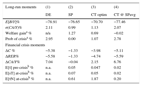
4.5

Simple financial policies

Given that the optimal financial policy is very effective but also very complex, it is important to consider the possibility that the policymaker may only have access to policy rules that are much simpler than the optimal policy. This raises the question of whether these simpler policies can still be effective. To shed light on this question, we compare the effects of the optimal policy with those produced by simple policies that restrict the policy instruments to be time- and state-invariant (i.e. constant taxes).

We consider two alternative simple policy rules. First, a rule that sets the constant policy rates equal to the long-run average rates under the optimal policy (denoted CT @ SPavg). Hence, under this simple rule the policy rates are set to (τ^N, s^T, τ) = (0.20, 0.02, 0.02) in percentages. The second simple rule corresponds to the triple (τ^N, s^T, τ) of constant policy rates that attains highest social welfare, in terms of expected lifetime utility (denoted CT @ optim). To find this triple, we use a derivative-free routine starting from the unregulated DE, in which (τ^N, s^T, τ) = (0, 0, 0). The resulting welfare-maximizing triple of constant policy rates is (τ^N, s^T, τ) = (1.87, 0.05, 0.047). The ergodic distributions produced by these simple rules are shown in Fig. 8, and the performance of these policies is compared with the optimal policy in Table 3.

Fig. 8.

Ergodic distributions of bonds with simpler policy rules.

Table 3.

Comparison of optimal v. simple policies.

Long-run moments	(1)	(2)	(3)	(4)
	DE	SP	CT optim	CT @ SPavg
E[B/Y]%	−78.91	−76.65	−70.70	−77.46
σ(CA/Y)%	2.11	0.99	1.13	2.07
Welfare gain^a %	n/a	1.27	0.69	−0.02
Prob of crisis^a %	2.95	0.00	1.07	2.78
Financial crisis moments
ΔC %	−5.38	−1.33	−3.98	−5.11
ΔRER%	−5.58	−1.33	−4.74	−5.59
ΔCA/Y%	7.04	−0.04	2.15	6.76
E[τ] pre-crisis^b %	n.a.	0.05	0.047	0.02
E[sT] at-crisis^b %	n.a.	0.07	0.05	0.02
E[τN] at-crisis^b %	n.a.	0.61	1.87	0.20

a

See notes on Table 2.

b

For the two simple rules with constant policy rates, the averages pre-crisis and at-crisis are the same as the unconditional averages by construction.

Fig. 8 shows that the ergodic distributions of bonds widen under the simple policy rules. As can be seen in Table 3, both of the simple rules reduce the average debt of the economy (i.e. increase NFA). However, agents are now less afraid of hitting the constraint, as shown by the position of the peaks in Fig. 8.

Table 3 shows that the simple rules we considered are significantly less effective than the optimal policy, and can even be welfare reducing. Relative to the DE, CT @ optim still yields a sizable drop in the probability of crises (from 3 to 1%), and it also reduces the severity of crises markedly (with smaller drops in consumption and the real exchange rate and a smaller current account reversal). Still, the optimal policy is significantly more effective in terms of reducing the frequency and magnitude of crises, and it yields a welfare gain that is about 60 basis points larger.

Constant policy rates set at the average of the optimal policy with CT @ SPavg rule are significantly inferior to both the optimal policy and the CT @ optim rule. Under CT @ SPavg, the probability of crisis is only slightly less than in the unregulated DE, the magnitude of crises is nearly unchanged, and in fact there is a small welfare loss of −0.02%. Hence, agents are worse off with this “poorly designed” financial policy than in the economy without any financial policy.

These results are in line with results obtained by Bianchi and Mendoza (2017). They found that simple rules for macroprudential debt taxes, in a model in which assets serve as collateral, are less effective than the optimal policy even when optimized to maximize welfare gains, and even allowing for time-varying, log-linear policy rules.

It is worth noting that the CT @ optim rule sets a constant debt tax and a constant subsidy for inputs used in the tradables sector that are similar to the values set under the optimal policy for the debt tax before crises and for the tradables subsidy during cries. In contrast, it sets a constant tax on inputs for the nontradables sector that is three times bigger than the crises average under the optimal policy. By doing this, the regulator with the CT @ Optim rule aims to prop up the relative price of nontradables more than under the optimal policy, and to do so permanently and not just when a crisis hits. This reduces the severity of crises when they happen, but also makes it less likely that the credit constraint can bind, and thus that crises can happen. On the other hand, the policy is inferior to the optimal policy because it induces misallocation of inputs across sectors at all times, instead of just during crisis events.

Fig. 9 shows event analysis windows that compare the macroeconomic dynamics of financial crises under the two simple policy rules and the unregulated DE. These plots illustrate again the result that the CT @ SPavg rule has negligible effects in terms of reducing the severity of crises. They also illustrate the mechanism by which the CT @ optim rule manages to do much better than CT @ SPavg mentioned earlier: When a crisis hits, it implies less severe declines in the relative price of nontradables and debt (recall that higher numbers in the graph for b′ indicate higher debt levels relative to the long-run average), and smaller current account reversals and consumption drops. Moreover, it also sustains higher debt levels at all times, since it reduces the likelihood of crises by propping up collateral values permanently.

Fig. 9.

Financial crisis events with simple policies.

5

Conclusions

This paper studied optimal financial policy in a liability dollarization model of financial crises driven by an occasionally binding collateral constraint. Agents in a small open economy have access to debt denominated in units of tradable goods, but face a constraint limiting their debt not to exceed a fraction of the market value of their total income also valued in units of tradables, which includes income from the tradables sector and income from the nontradables sector valued at the equilibrium relative price of nontradables (i.e. the real exchange rate). Similar models have been widely used to study macroprudential policy, because they embody a pecuniary externality that justifies policy intervention. In particular, in normal times agents do not internalize the effect of their borrowing decisions on the size of the collapse in the price of nontradables, and hence on the collapse in collateral values and borrowing capacity, in crisis times.

The model we studied is based on the model proposed by Bianchi et al. (2016). They examined a liability dollarization model driven by conventional and unconventional shocks, with the latter including fluctuations across regimes of global liquidity (e.g. a regime-switching specification of world interest rate shocks) and noisy news about fundamentals (e.g. news about future tradables income). We modified the Bianchi et al. model by introducing production of tradable and nontradable goods using intermediate goods.

Introducing production has important implications for the optimal design of financial policy. In particular, the optimal policy has both a macroprudential (ex-ante) component, which has the standard property of being active only when the collateral constraint does not bind contemporaneously but may bind in the following period with some probability, and ex-post components that are active only when the collateral constraint binds. The macroprudential component is modeled in the familiar form used in the literature, as a debt tax that increases the private marginal cost of borrowing to match the social cost in normal times. The ex-post components take the form of a tax on input purchases levied on producers of nontradables, and a subsidy on input purchases provided to producers of tradables. These two instruments reallocate production across sectors so as to prop up collateral values and hence borrowing capacity in crisis times.

The model was calibrated using Colombian data, and a set of quantitative experiments showed that, while optimal financial policy is a very effective tool for reducing the frequency and severity of financial crises, it is also a very complex policy that entails significant, non-linear variation in policy instruments over time and across states of nature. In addition, the paper shows that if only simple policy rules in the form of time- and state-invariant policy instruments are feasible, these simple rules are at best much less effective than the optimal policy and at worst they can result in lower welfare than in an economy in which financial crises occur without policy intervention.

The findings of this paper indicate that the implementation and design of policies aimed at tackling financial instability should proceed with caution. In particular, specific policy rules need to be the subject of intensive quantitative assessment with macroeconomic models that capture the relevant transmission mechanisms that drive financial crisis and the transitions from normal to crisis times, because otherwise seemingly harmless simple rules can actually be welfare-reducing.

Conflict of interest

The authors declare no conflict of interest.