Credit and business cycles: Causal effects in the frequency domain

Abstract

The history of economic recessions has shown that every deep downturn has been accompanied by disruptions in the financial sector. Paradoxically, up until the financial world crisis of 2007–2009, little attention was given to macroeconomic and financial interdependence. In this paper, a study is conducted on the relationship between financial and real business cycles for a sample of thirty-three countries in the frequency domain. Specifically, the features of the interdependence of credit and output cycles are analysed and Granger-type causality tests are carried out in the frequency domain. The main findings of the study indicate that the likelihood of cycle interdependence is highest when considering medium and long-term frequencies, and that Granger causality runs in both directions.

Resumen

Tradicionalmente, las recesiones han venido acompañadas de disrupciones importantes en el funcionamiento del sistema financiero. Paradójicamente, antes de la crisis financiera de 2007-2009 se daba muy poca importancia a la interdependencia entre la macroeconomía y el sistema financiero. En este documento estudiamos la relación entre ciclos financieros y ciclos de producto para una muestra de treinta y tres países. Específicamente, caracterizamos la interdependencia entre estos ciclos y realizamos pruebas de causalidad tipo Granger en el dominio de la frecuencia. Nuestros resultados principales indican que la mayor interdependencia ocurre en frecuencias asociables al mediano y largo plazo. Encontramos evidencia de causalidad bi-direccional.

1

Introduction

The history of economic recessions has shown that every deep downturn has been accompanied by disruptions in the financial sector. Paradoxically, up until the recent financial world crisis, the linkage between financial and macroeconomic variables remained almost entirely unexplored. Recently, a small but growing literature has surfaced regarding the importance of the financial sector and its role on the business cycle. Examples include Cúrdia and Woodford (2010), Christiano, Motto, and Rostagno (2010), Claessens, Kose, and Terrones (2012), Drehmann, Borio, and Tsatsaronis (2012), Gertler and Kiyotaki (2010), Hafstead and Smith (2012), Meh and Moran (2010), and Schularick and Taylor (2012). Notwithstanding, significant effort is still needed in order to attain a comprehensive understanding of the causal links between the financial sector and the macroeconomy.

In this paper we extend the work of Gomez-Gonzalez, Ojeda-Joya, Zárate, and Tenjo-Galarza (2014) to study the relationship between financial and output cycles for thirty-three countries in the frequency domain. Our sample includes both developed and emerging market economies which allow us to make several benchmark comparisons. While the literature has mainly focused on developed economies, little is known about cycle interdependence for emerging markets. Thus, our paper intends to shed some light on the latter and serve as a building block for the construction of future theoretical models.

Our contributions to the literature are two-fold. First, we characterize the interdependence of credit and output cycles in the frequency domain, sidestepping the need of assumptions regarding which frequency to select in the data. Hence, in contrast to most of the existing literature, our study avoids issues that center on the differences between different time horizons of cycles (see Drehmann et al., 2012). Second, following the methodology presented in Breitung and Candelon (2006), we perform Granger-type causality tests in the frequency domain. By doing so, we obtain stronger results than if using cross-correlation coefficients. Our paper confirms some of the previous findings from the literature but also uncovers new results. Similar to Borio (2011) and Drehmann et al. (2012), we find that the likelihood of cycle interdependence is highest when considering medium and long-term frequencies. However, in contrast to most of the related literature, we find that Granger causality runs in both directions.

2

Literature review

2.1

Early studies

According to Minsky's instability hypothesis, financial cycles systematically affect real business cycles. The former is an endogenous result of when firms transition from a hedge finance scheme towards a purely speculative (or Ponzi finance) scheme. ¹

Financial instability is then hightened during long periods of economic tranquility. In good times, the economy grows at a steady pace in which credit defaults are rare and risk-taking incentives are heightened. Examples include prolonged periods of loose monetary policy, often leading to the search for different yield strategies. As a result, firms and households’ risk tolerance increase (bearing higher levels of debt) while private banks lower their lending standards. Higher profit expectations shift the debt structure of firms towards Ponzi finance schemes, increasing investment even further. ² Similarly, higher income increases households’ debt-to-income ratio.

In the related literature, there is strong support of this behavior in booming periods, as seen in Amador, Gómez-González, and Murcia (2013), Asea and Blomberg (1998), Figueroa and Leukhina (2010), Weinberg (1995), and Kaufmann and Scharler (2013).

2.2

Recent literature

In contrast with earlier studies, the recent literature's dominant approach has consisted of modeling financial frictions; embedded in a dynamic stochastic general equilibrium (DSGE) framework. These models build on the financial accelerator model developed by Bernanke and Gertler (1989), and extended by Carlstrom and Fuerst (1997), Kiyotaki and Moore (1997) and Bernanke, Gertler, and Gilchrist (1999). Overall, this strand of literature emphasizes the role of financial intermediaries and characterizes structural shocks that affect the borrowing and lending process.

There are numerous renowned examples. For instance, Cúrdia and Woodford (2010) study the desirability of modifying a standard Taylor rule by incorporating variations in credit spreads and credit quantities. Christiano et al. (2010) model financial contracts and liquidity constraints by introducing financial markets and a banking sector. Similarly, Meh and Moran (2010) include a banking sector in order to solve for information problems between banks and creditors (involving differences in the level of capital). Gertler and Kiyotaki (2010) build a hybrid model based on Gertler and Karadi (2013) and Kiyotaki and Moore (1997) to allow for financial intermediation and liquidity risk. The authors show how disruptions in intermediation can induce a crisis, and how credit market interventions can help mitigate one. Hafstead and Smith (2012) develop a financial accelerator model in which a monopolistically competitive banking sector is introduced, and an interbank market exists. The authors find that shocks originating in the financial sector can have large macroeconomic effects and that monetary policy plays an important role in mitigating them.

In sum, the recent growth in the literature has yielded important results vis-à-vis its critics. For instance, Del Negro, Giannoni, and Schorfheide (2013), estimate a standard New Keynesian model with financial frictions that predicts the recent world crisis of 2009. However, it is worth noting that some authors advocate for the use of different modeling techniques. For instance, Borio (2011) recalls for a reconsideration of the prevailing paradigm embedded in macroeconomics. Particularly, he dissents from a rediscovery of the monetary nature of modern economies, in which inside credit creation plays a major role.

3

Frequency domain analysis

The frequency domain approach is implemented in three stages. First, we estimate the spectral function of each variable. This estimation allows comparing the shape of the spectral density with the “typical shape” identified in Granger (1966). Second, we use the direct filter approach to extract cycles using Fourier analysis.³ Finally, we estimate the co-movement between cycles by using the cross-spectral density function and its related measures of coherence.

This methodology is conducted for the entire frequency range (0 to π). This approach allows estimating the proportion of the total variance determined by each periodic component. Therefore, we capture the components of credit and output by decomposing the original series and using approximation methods based on trigonometric functions at each frequency. Signal extraction techniques are based on smoothing filters (Christiano & Fitzgerald, 2003) and modeling-based procedures. However, the components of the time series give rise to spectral structures that fall within well-defined frequency bands (isolated from each other by spectral dead spaces).⁴ Thus, the frequency domain offers a better way of implementing signal extraction methods, and filters are used to separate the components of time series.

The autocovariance function of the Fourier transformation is given by the following symmetric function:

where ω is the frequency in radians in the range −π,π. The standardized function, known as the spectral density, is obtained by normalizing Eq. (1) by using γ0. A cycle is defined as a unit period of a sine or cosine function over a time interval of length 2π .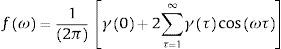

It is important to note that the spectrum and the covariances are equivalent. However, some features of time series, such as serial correlation, are easier to grasp using autocovariances. Others, such as unobserved components, are easier to analyze using the whole spectrum.

Values of ω near zero correspond to long-term cycles, while values of ω near π correspond to short-term cycles. The peaks observed in the spectrum indicate those periodicities which contribute the most to the variability of the series. Additionally, confidence intervals for the spectrum can be obtained from the fact that fω follows a χ² distribution with ν degrees of freedom (where ν=3n1/22, and n stands for the sample size).

The direct filter approach (DFA) emphasizes on filter errors rather than on the one-step ahead forecasting error. Furthermore, the DFA uses an algorithm based on an optimization criterion which consists of minimizing the mean square error of the filter.

Given a stochastic process Yt, the real time signal extraction is concerned with the estimation of Yˆt and Y¯t such that EY¯t−Yˆt2 is minimized. In this context, Y¯t is the result of applying a symmetric filter to the original series, while Yˆt is the result of applying an asymmetric filter.

The result of this minimization is a transfer function, Γω, which can be used as a filter. One particular application which we use in this study is the filter proposed by Christiano and Fitzgerald (2003):

where b_p determines the width of the pass band and b_s determines the width of the stop band (see Wildi, 2008).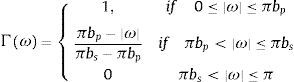

The cross-spectral correlation function measures the correlation between two series indexed by the frequency. The square of the value of this correlation function at every frequency ω is defined as its coherence. This statistic is the analogous of the square of the correlation coefficient and takes on values in the interval [0, 1]. A value of coherence near one indicates that the two series are highly associated at the given frequency. A value near zero describes that at this frequency the series are almost independent.

3.1

VAR setup

In order to test for causality between GDP and Credit cycles in the frequency domain, we use the measures proposed by Geweke (1982) and Hosoya (1991) and adopted by Breitung and Candelon (2006) in a VAR system setup.

Let Zt=GDPt,CREDITt be a two dimensional vector of time series observed for t = 1, 2, ⋯ T, which represents the total cycle of these two variables.⁵ Thus, the VAR representation of this system can be expressed as in Eq. (3):

The moving average (MA) representation of the system is the following:

Where

And G is the lower matrix of Cholesky decomposition. Using this representation, the spectral density of GDP_t, for example, can be expressed as: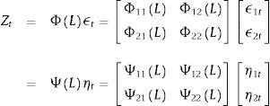

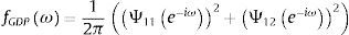
From the above expression, and following Breitung and Candelon (2006), the measure of causality is defined as:

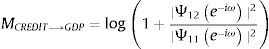
This causality measure is zero if Ψ12e−iω2=0, which means that the variable CREDIT does not cause GDP at frequency ω. The causality of GDP to CREDIT is built using a similar approach.

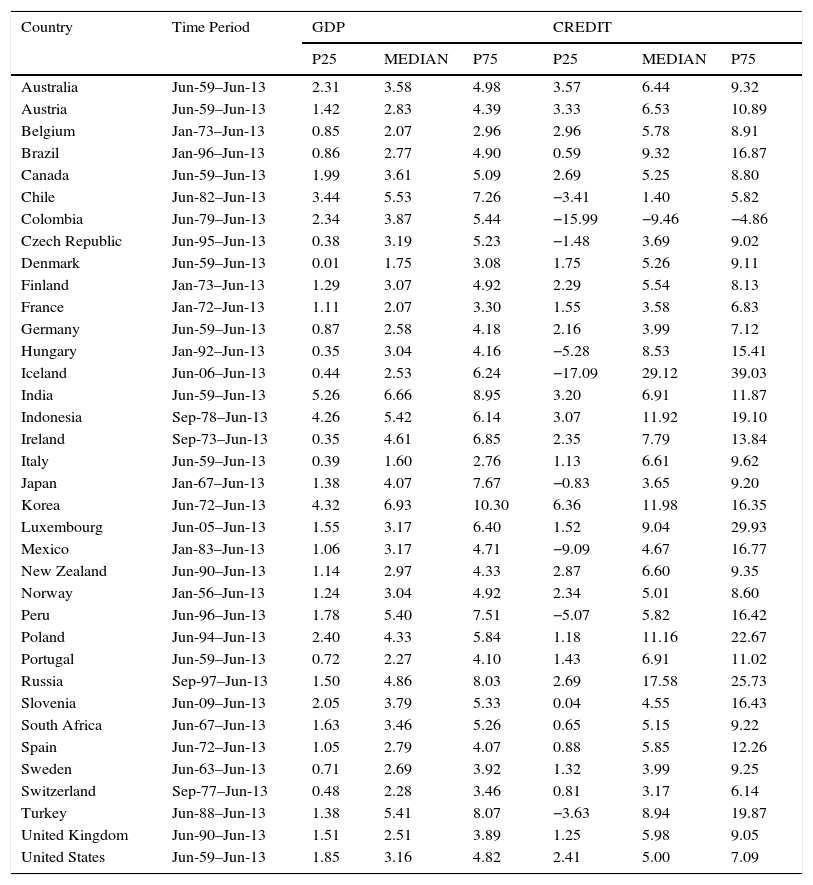
4

Data

Our dataset (quarterly frequency) consists of credit to the private non-financial sector and real GDP for 33 economies.⁶ Following Aikman, Haldane, and Nelson (2011), Jordà, Schularick, and Taylor (2011), Schularick and Taylor (2012), we use the credit cycle as a proxy for the financial cycle. In spite of a general lack of consensus on its exact definition, some studies have shown that the most parsimonious definition of the financial cycle is in terms of credit.⁷ Most data on credit, adjusted for breaks, were obtained from the Bank for International Settlements (BIS). For countries not included in the BIS database (namely Colombia, Chile and Peru) we collected official data from each central bank. All observations on variables were collected for the longest available period, ranging from the early 1940s until the second quarter of 2013 (see Appendix 1 for a summary of descriptive statistics for each country). The nominal GDP and the Consumer Price Index (CPI) were both obtained from the International Financial Statistics database of the International Monetary Fund. All data used in this study are expressed in constant prices (using the CPI of each country as deflator).⁸

Appendix 1.

Summary statistics.

Country	Time Period	GDP			CREDIT
		P25	MEDIAN	P75	P25	MEDIAN	P75
Australia	Jun-59–Jun-13	2.31	3.58	4.98	3.57	6.44	9.32
Austria	Jun-59–Jun-13	1.42	2.83	4.39	3.33	6.53	10.89
Belgium	Jan-73–Jun-13	0.85	2.07	2.96	2.96	5.78	8.91
Brazil	Jan-96–Jun-13	0.86	2.77	4.90	0.59	9.32	16.87
Canada	Jun-59–Jun-13	1.99	3.61	5.09	2.69	5.25	8.80
Chile	Jun-82–Jun-13	3.44	5.53	7.26	−3.41	1.40	5.82
Colombia	Jun-79–Jun-13	2.34	3.87	5.44	−15.99	−9.46	−4.86
Czech Republic	Jun-95–Jun-13	0.38	3.19	5.23	−1.48	3.69	9.02
Denmark	Jun-59–Jun-13	0.01	1.75	3.08	1.75	5.26	9.11
Finland	Jan-73–Jun-13	1.29	3.07	4.92	2.29	5.54	8.13
France	Jan-72–Jun-13	1.11	2.07	3.30	1.55	3.58	6.83
Germany	Jun-59–Jun-13	0.87	2.58	4.18	2.16	3.99	7.12
Hungary	Jan-92–Jun-13	0.35	3.04	4.16	−5.28	8.53	15.41
Iceland	Jun-06–Jun-13	0.44	2.53	6.24	−17.09	29.12	39.03
India	Jun-59–Jun-13	5.26	6.66	8.95	3.20	6.91	11.87
Indonesia	Sep-78–Jun-13	4.26	5.42	6.14	3.07	11.92	19.10
Ireland	Sep-73–Jun-13	0.35	4.61	6.85	2.35	7.79	13.84
Italy	Jun-59–Jun-13	0.39	1.60	2.76	1.13	6.61	9.62
Japan	Jan-67–Jun-13	1.38	4.07	7.67	−0.83	3.65	9.20
Korea	Jun-72–Jun-13	4.32	6.93	10.30	6.36	11.98	16.35
Luxembourg	Jun-05–Jun-13	1.55	3.17	6.40	1.52	9.04	29.93
Mexico	Jan-83–Jun-13	1.06	3.17	4.71	−9.09	4.67	16.77
New Zealand	Jun-90–Jun-13	1.14	2.97	4.33	2.87	6.60	9.35
Norway	Jan-56–Jun-13	1.24	3.04	4.92	2.34	5.01	8.60
Peru	Jun-96–Jun-13	1.78	5.40	7.51	−5.07	5.82	16.42
Poland	Jun-94–Jun-13	2.40	4.33	5.84	1.18	11.16	22.67
Portugal	Jun-59–Jun-13	0.72	2.27	4.10	1.43	6.91	11.02
Russia	Sep-97–Jun-13	1.50	4.86	8.03	2.69	17.58	25.73
Slovenia	Jun-09–Jun-13	2.05	3.79	5.33	0.04	4.55	16.43
South Africa	Jun-67–Jun-13	1.63	3.46	5.26	0.65	5.15	9.22
Spain	Jun-72–Jun-13	1.05	2.79	4.07	0.88	5.85	12.26
Sweden	Jun-63–Jun-13	0.71	2.69	3.92	1.32	3.99	9.25
Switzerland	Sep-77–Jun-13	0.48	2.28	3.46	0.81	3.17	6.14
Turkey	Jun-88–Jun-13	1.38	5.41	8.07	−3.63	8.94	19.87
United Kingdom	Jun-90–Jun-13	1.51	2.51	3.89	1.25	5.98	9.05
United States	Jun-59–Jun-13	1.85	3.16	4.82	2.41	5.00	7.09

Source: Authors’ calculations. P25 and P75 correspond to the bottom 25% and top 75% values, respectively.

5

Empirical results

Figs. 1–3 illustrate our main results based on coherence statistics, cross-correlations in the frequency domain and Granger causality tests, respectively. In order to improve readability and to allow a comparison of our results with previous studies, we transformed the frequency domain into time intervals (quarters), using the following function:

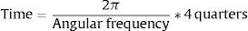
Consequently, we followed Drehmann et al. (2012) to establish conventional duration horizons for short (5–32 quarters), medium (32–80 quarters) and long-term (more than 80 quarters) cycles.

Fig. 1 shows results of computing coherence statistics between credit and GDP for all 33 countries. High values of coherence correspond to a high correlation between credit and GDP. Results show that credit and GDP cycles appear to have greater correlation at medium and long-term frequencies for most countries in our sample (29 out of 33). This fact highlights the importance of looking at medium and long-term credit cycles when designing macro-prudential policies. The only exceptions include Belgium, India, Mexico and Peru, for which the greater values of coherence occur at short-term frequencies.

Fig. 1.

Coherence Statistics between GDP and Credit by Country (Frequency Domain – Horizontal axis measured in quarters).

Fig. 2 depicts the cross-correlation between credit and GDP. Each sub-figure comprises the correlation between credit lags and contemporaneous GDP (negative values on the horizontal axis) as well as the correlation between GDP lags and contemporaneous credit (positive values on the horizontal axis) for the whole frequency spectrum. All countries (except Korea) exhibit global maxima at the left hand-side of the domain, indicating a positive relationship between lags in credit and contemporaneous output, specially marked in frequencies corresponding to the medium term. Conversely, all countries present a global minimum at the right hand-side of the domain. This is evidence of a negative correlation between GDP lags and contemporaneous credit, again with a higher influence over the medium term. In sum, credit cycle peaks precede booms in output, while peaks in the output cycle precede troughs in the credit cycle. This result corroborates the findings obtained by Schularick and Taylor (2012).

Fig. 2.

Cross-correlations in the frequency domain between GDP and Credit by Country (Angular frequency in horizontal axis- vs. Correlation Coefficient in vertical axis). The two points marked in each graph are the maximum correlations from lagged GDP to contemporaneous Credit and vice-versa.

Fig. 3 depicts results for Granger causality tests between credit and GDP, based on the methodology proposed by Breitung and Candelon (2006). We performed this test for the 33 countries in our sample and for the two directions of causality.⁹ Therefore, Fig. 3 consists of 66 sub-figures. The horizontal line represents the critical value at the 95% significance level (values above the critical value indicate causality at a given frequency). Results show that causality runs in both directions (stronger in medium and long-term frequencies), for most casas. There is however, some heterogeneity among countries. For instance, there are countries like Peru for which causality runs in only one direction. Finally, medium and long-term causality is the most evident.

Fig. 3.

Causality Tests by Country in the Frequency Domain (Quarters in the horizontal axis vs. Statistic of Granger's Causality Test in the vertical axis). The horizontal line in each of the graphs represents the critical values for the Granger's causality test. Angular frequency values above it suggest that variables in these frequencies cause one another.

Our findings shed light on salient features of macroeconomic modeling. The relationship between financial and real variables is complex, and financial factors influence economic activity beyond exogenous shocks. Overall, we illustrate that GDP and credit cycles are not perfectly synchronized. The relationship between these two cycles is stronger when lags are included. An interesting implication for monetary policy is that it is difficult to target both financial and real variables using just one instrument. Moreover, credit should not be ignored when the objective is to stabilize the economy, as credit cycles exert important influence over the business cycle, and vice-versa.

These results are similar to those found in Drehmann et al. (2012) in the sense that financial cycles are mostly related to business cycles in the medium-term. In our sample, these results hold true for developed countries such as Australia, Germany, Japan, Norway, Sweden, United Kingdom and the United States. However, while Drehmann et al. (2012) focus on the time domain, our focus lies in the frequency domain. Our study also focuses on Granger-type causality tests instead of conducting correlation analysis.

6

Conclusions

We study the relationship between financial and real business cycles for thirty-three countries in the frequency domain. Our sample includes both developed and emerging market economies which allow us to make several benchmark comparisons. We contribute to the literature by first, characterizing the interdependence of credit and output cycles in the frequency domain. In contrast to most of the existing literature, our study avoids issues that center on the differences between short and long-term analysis of cycles. Second, we perform Granger-type causality tests in the frequency domain. By doing so, we obtain stronger results than studies using cross-correlation coefficients.

Our paper confirms some of the previous findings from the literature but also uncovers new results. Similar to Borio (2011) and Drehmann et al. (2012), we find that the likelihood of cycle interdependence is highest when considering medium and long-term frequencies. However, in contrast to most of the related literature, we find that Granger causality runs in both directions.

As such, monetary authorities can benefit by focusing on medium and long-term credit cycles when designing macro-prudential policies. Moreover, credit cycles should be carefully analyzed when trying to stabilize the economy, as they exert important influence over the business cycle, and vice-versa. We believe that our findings elicit key structural differences between emerging and developed economies that can potentially serve as building blocks for the construction of future theoretical models.

Conflict of interests

The authors declare no conflict of interest.