A model of medium term exchange rate forecast in an open economy The case of the mexican peso

Abstract

Keynes (1930) and Samuelson (1965) proposals open the possibility of matching predictability and efficiency, as evidenced by the seminal study by Fisher (1930). Recent findings suggest that the foreign exchange market gradually incorporates relevant information allowing the formation of prices in a rational manner but not randomly. Models of exchange rate by term based on asset valuation suggest that the inclusion of risk in the spot rate increases the degree of predictability. The results show that after incorporating an accurate measure of risk, predictability of medium term foreign exchange rate increases.

Resumen

Las propuestas de Keynes (1930) y Samuelson (1965) abren la posibilidad de compatibilizar eficiencia con predictibilidad según se deduce del estudio seminal de Fisher (1930). Recientes hallazgos sugieren que el mercado de divisas incorpora gradualmente la información relevante favoreciendo la conformación de precios de manera racional y no aleatoria. Los modelos del tipo de cambio a plazo basados en la valuación de activos sugieren que la inclusión del riesgo al tipo de cambio spot aumenta el grado de predictibilidad. Los resultados muestran que tras incorporar una medida precisa de riesgo se aumenta sustancialmente la predictibilidad del tipo de cambio en el mediano plazo.

Introduction

The FOREX market is the most important financial market in the world, its daily trading volume of negotiation impacts on the behavior of other financial markets or those of goods and services. More recent data show that the daily volume of trade hits 9 trillion dollars, which exceeded by more than one hundred times the daily average value of Wall Street shares.

Therefore, it is a very profitable market. Since the FOREX market liberalization and the adoption of the system of flexible exchange rate, in 1973, exchange rates have become increasingly erratic and volatile. That is why it is frequent that corporate decisions are increasingly adopting exchange rate forecasting techniques. Even speculative positions, protectionist or arbitrage of investors have to take into account the behavior of exchange rates.

The literature shows studies that begin to explain, not only the composition of the current exchange rates, but to find those elements that determine their value over time. So, for more than a century, economists have tried to establish and then model the factors that determine the exchange rate. Economic literature precisely documents the existence of five theories that explain the determinants of exchange rate. One of these models assumes efficient markets, and then equilibrium is always achieved. Although in the practice, it is a fact difficult to achieve due to arbitrage operations (Eun and Resnick, 2007).

The latter point brings an interesting discussion: Either exchange rates are given at random or by irrational movements given that operators are involved in efficient markets or, investors make rational decisions that allow them to take advantage of arbitrage opportunities. The certainty of the term arbitrage opportunities will depend on the robustness of the exchange rate forecasts.

In this regard, one of the first studies on exchange rate arbitrage conditions term was proposed by Samuelson (1965) and empirically developed by Cornell and Dietrich (1978) without conclusive results achieved in their models. At that time the common denominator of these studies was to consider the theoretical forward rate as an unbiased predictor of the exchange rate term. However, the seminal work of Messe and Rogoff (1983) showed the poor predictive ability of models to determine the exchange rate compared to a naive random walk model (random walk). Since then there has been an enormous effort to both deepen and unravel the causes of the extreme difficulty of forecasting exchange rates. They also provided alternative procedures of some predictive improvement over the random walk model.

Thus, recent models suggest that the inclusion of risk prediction models to the exchange rate will provide more robust models, but for this, it is essential to capture it properly. We will develop our model by following the line of the latter approach.

This study has been divided into four sections. The following section gives particular attention on models based on assets valuation thus giving rise to the third section that analyzes the statistical robustness according with the classical risk models that will permit conclusions at the end.

Different approaches

Basic approaches about exchange rate predictions

Asymmetries frequently come in profitable arbitrage operations, therefore, this value will fluctuate not only between the contributions that are being made in different currencies (spot market), but will also change over time. Thus, exchange rate is given by the ratio of one currency against another in the following way:

Where, Q_A refers to the number of units of currency A required to convert in terms of currency B, and 1_B refers to the counter-currency.

For more than a century, economists have tried to establish and model the factors that determine the exchange rate¹. Recent theories that show better result are those based on assets valuation, due to their ability to explain the behavior of exchange rates from monetary market expectations for inflation and interest rates. There are various models developed within this approach which vary only in the degree of recognition of their impact on exchange rates.

In practice, companies generate their own forecasts, while others pay specialized firms to do the job. Forecasting techniques would be classified in any of the following approaches: a) Efficient Market Model, b) Technical or Chartist Model and c) Economic or Fundamental Model. Table 1 collects the main features of the models above.

Table 1.

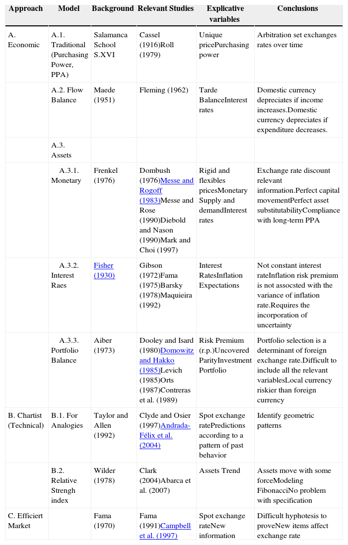
Most relevant studies about the behavior of the exchange rate

Approach	Model	Background	Relevant Studies	Explicative variables	Conclusions
A. Economic	A.1. Traditional (Purchasing Power, PPA)	Salamanca School S.XVI	Cassel (1916)Roll (1979)	Unique pricePurchasing power	Arbitration set exchanges rates over time
	A.2. Flow Balance	Maede (1951)	Fleming (1962)	Tarde BalanceInterest rates	Domestic currency depreciates if income increases.Domestic currency depreciates if expenditure decreases.
	A.3. Assets
	A.3.1. Monetary	Frenkel (1976)	Dombush (1976)Messe and Rogoff (1983)Messe and Rose (1990)Diebold and Nason (1990)Mark and Choi (1997)	Rigid and flexibles pricesMonetary Supply and demandInterest rates	Exchange rate discount relevant information.Perfect capital movementPerfect asset substitutabilityCompliance with long-term PPA
	A.3.2. Interest Raes	Fisher (1930)	Gibson (1972)Fama (1975)Barsky (1978)Maquieira (1992)	Interest RatesInflation Expectations	Not constant interest rateInflation risk premium is not assocsted with the variance of inflation rate.Requires the incorporation of uncertainty
	A.3.3. Portfolio Balance	Aiber (1973)	Dooley and Isard (1980)Domowitz and Hakko (1985)Levich (1985)Orts (1987)Contreras et al. (1989)	Risk Premium (r.p.)Uncovered ParityInvestment Portfolio	Portfolio selection is a determinant of foreign exchange rate.Difficult to include all the relevant variablesLocal currency riskier than foreign currency
B. Chartist (Technical)	B.1. For Analogies	Taylor and Allen (1992)	Clyde and Osier (1997)Andrada-Félix et al. (2004)	Spot exchange ratePredictions according to a pattern of past behavior	Identify geometric patterns
	B.2. Relative Strengh index	Wilder (1978)	Clark (2004)Abarca et al. (2007)	Assets Trend	Assets move with some forceModeling FibonacciNo problem with specification
C. Efficiert Market		Fama (1970)	Fama (1991)Campbell et al. (1997)	Spot exchange rateNew information	Difficult hyphotesis to proveNew items affect exchange rate

The model based on efficient market, considered by many as a purely theoretical assumption (see Campbell et al., 1997), has had an enormous influence on financial studies of assets valuation, including exchange rate issue. The latter model is based on the idea of Fama (1970) where it is assumed that all the information is relevant and discounted by the agents. Thus, the current exchange rate will reflect all the relevant information, such as inflation, trade balance, economic growth and money supply conditions; then, the exchange rate would be affected only if it receives new information, even if unexpected. As a result, the new exchange rate is fixed independently of its historical performance. From this perspective, it is not surprising that the exchange rate follow a random walk and, therefore, the current exchange rate would be the best predictor of the exchange rate term (Fwtt+1). Hence the predictor is defined as:

Where I_t is the available information, Fwtt+1 is the theoretical forward exchange rate, S_t+1 is the spot exchange rate at maturity. In general, it is assumed that differences between interest rates causes that exchange rate Fwtt+1 vary with respect to the current exchange rate.²

In addition, another model called “Chartist”, based on the approach of Caballer (1998) and efficient market establishes that information is automatically reflected in price and therefore does not justify the development of previous studies, i.e.: “If I have no idea of the value of a company, but others more powerful than me have it and those big, acting in the market, leave a trail of their conclusions I can reach their own conclusions” (Elliot et al., 2000: 47). This approach analyzes figures and statistical charts to anticipate the movement of the currency. Following this line of research, several indicators have been designed (such as RSI, Fibonacci) to predict, with acceptable accuracy, the trend and strength of the currency. It has been accepted, by the academic community, that the use of these tools determines the timing of investment or asset sale (Andrada-Félix et al., 2004).

However, between these different approaches, the best predictor can be based on economic fundamentals. This is because the economic agent is rational given that the relevant information is being gradually introduced to the expectations of investors. In the next section, we will study advanced approaches to build up our own model to find the best exchange rate predictor.

The forward exchange rate under models based on asset valuation

The classical theory is based on asset valuation which begins by calculating the points pips to be added to the spot rate in order to find the forward exchange rate, i.e.,

We can see that the predictive accuracy is subject to exchange rate fluctuations with the spot rate (S) at maturity, i.e., at the time of the operation. Moreover, improving the timing problem detected in Fisher's classical model (1930), the general equation may be specified by:

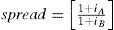
Where, n is the forward term in days; spread is the differential between the interest rates of the currencies on each country, i.e. pips have to add or subtract the current exchange rate; here the interest rates should match the exchange rate term calculated in the forward. In any case, differential in interest rates represents the gap between the interest rate in country A (i_A) and the interest rate in country B (i_B), i.e.,

Kozikowzki (2000) shows an adjustment to the formula (4) that captures difference in rates and terms³:

Table 2.

Goodness contrast of the classical predictors MXP/USD using DM

Simulated exchange Rate Fw	Ec (3)	Ec (4)	Ec (6) Componente
Sept-2009	5.5752 **	1.932	6.8292 **
Oct-2009	1.0209	−0.9432	2.30922 *
Nov-2009	5.2002 **	1.726	−0.928
Dec-2009	1.0912	−0.5287	0.8427
Jan-201	5.6039 **	3.72628 *	3.6373 *

**

Significant to 1%

*

Significant to 5%

Anomalies and risk premiums

Financial economists have extensively analyzed whether the currency forward markets reflect all relevant information. In this sense, in an environment without arbitrage, the assumptions of risk neutrality and rational expectations lead to believe that the interest rate should be an unbiased predictor of forward exchange rates (Ai). This assertion has been called unbiased forward exchange rate Hypothesis (UFER).

From the beginning, we have the following specification to test the UFER:

Even though the null hypothesis established in equation (10) defines the conditions of equation (11), i.e., α = 0, β = 1, subsequent investigations about unit root tests (unit roots) have raised serious doubts about the properties of equation (11), as the conventional wisdom about the behavior of unit root would continue to exchange rates. This concern about spurious regressions prompted researchers to explore alternatives such as stationary behavior in equation (11)⁴ that led to the following equation:

Where ΔlnABA=(lnABA−lnSBA). The early estimates were based on this equation (8) that continued to reject the UFER both in tests of forward exchange rates at various maturities as in experiments that used different currencies. In this situation, the studies showed findings regarding the paradox of capital premium, contradicting, this way, Fisher's classical theory that assumed the positions of the premium or discount affecting prices under the same pattern. At bottom, it seems unlikely that the simple rule of investing in the highest rate guarantees good results and be predictive and, then, it is an issue that has not been tested or fully explored. Although an interesting finding of this research is to obtain frequent βˆ negative estimates⁵. A βˆ negative means that investors would be happy to invest in currencies with higher interest rate.⁶ See table 3 that shows the results of testing the dispersion of forward exchange rate as a predictor of the spot exchange rate.

Table 3.

Estimation of spread in the Forward Exchange Rate

ΔlnABA=α+β(lnFwtt+1−lnSBA)+ϵt+1
Works	Period	Counties	β˙	Significance level of 5%
Fama (1984)	1973–32	Japan	−0.29	No
		Switzerland	−1.14	No
		United Kingdom	−0.90	No
		Canda	−0.87	No
Barnhart and Szakmary (1991)	1974–88	Germany	−3.63	Yes
		United Kingdom	−1 65	Yes
		Japan	−0.59	No
		Canada	−2.02	Yes
Bekaert and Hodrick (1993)	1975–89	Germany	−3.015	Yes
		United Kingdom	−2.021	Yes
		Japan	−2.098	Yes

Researchers have come to conclude that the inconsistencies found in a recent connection to the classical theories on exchange rates could be due to economic factors irrelevant to attract the attention of speculators and therefore difficult to detect. As a result, it raises an interesting possibility to find this relationship in which the inclusion of risk would be given depending on the behavior and level of interest rates of the currencies involved.

The possibility of a premium

With little strength on the empirical findings on the UFER, Fama (1984) and Nieuwland et al. (2000) are only a few attempts to reconcile the anomalous results found in practice with efficient market theory. The existence of a risk premium for them would be the variable that would explain the exchange rate term. The argument is that risk aversion investors have required compensation to motivate them to take that risk, and after relaxation of the neutrality that could be at risk while maintaining the rationality, the formation of expectations denote as follows:

Equation (8) emphasizes the importance of detecting the presence of a risk premium ρ_t, capturing many economic relations, theory often prescribes those variables that are unobservable. This observation is important because while economic models can be considered robust when they incorporate risk premiums, failing to detect the risk premium means that these models are inadequate rather than when they provide information without considering the premium.

For this reason, researchers have been focusing, through numerous techniques for the detection of a risk premium in the forward market. For example, Barnhart and Szakmary (1991) incorporated Kalman filter extraction method which approaches signals, detecting some deterministic components in the error. According to their findings, the error can be characterized in an AR (1) which can be removed with systematic patterns. However, the presence of a systematic component is not sufficient to conclude that this bias compensates the risk of speculation agents down because they would be leaving out the formation of rational expectations. However, the method proposed by Barnhart and Szakmary (1991) cannot determine the possibility of risk compensation because it does not explain the increase in predictability.

In this regard the Engel's seminal work (1982) on autoregressive conditional heterocedasticity (ARCH)-which initially was used to verify if the volatility of the forecast error could explain the assumptions about the behavior of interest rates, resulted in ARCH-type models in the mean (ARCH-M), and would be useful to identify and analyze the performance of financial assets during periods of turbulence but also of peace. Among the conclusions in this type of works it is shown that a greater variation in yields creates a greater climate of uncertainty for investment, so investors with some degree of risk aversion will demand compensation for the above average during the periods of uncertainty. Domowitz and Hakkio (1985) found that after a certain level in the conditional variance by investors, there is an increase in risk premiums as compensation rises.

In this sense, the ARCH-M model detects the influence of conditional volatility on the conditional mean and, therefore, can measure the expectations and influence of stakeholders on higher risk premiums in more turbulent times. However, Domowitz and Hakkio (1985), Baillie and Bollerslev (1990) and Bekaert and Hodrick (1993) found little evidence to reinforce the idea that the premium depends on the conditional variance of error in the forecast. Fundamentally, the sense of volatility has been the limiting factor for explaining abnormality. It is true that agents, acting on both sides of the market, are subject to the same volatility but that volatility alone cannot explain what makes a premium currency. Then, the ARCH-M model does not explain why a currency attracts premium⁷ as a natural progression of the issue would be to explain the relationship that exists between the systematic risk and the participant's expectations in the currency market.

Systematic risk and the risk premium

It has been found that the Fisher effect generates a non-symmetrical relation between nominal interest rates and increased inflation. Consequently, the real interest rate does not correspond to the risk-free rate, since it incorporates other types of risk. The articles that studied the relationship between systematic risk and the risk premium do not make explicit why a currency attracts premium as it does. Cumby (1988) and Kaminsky and Peruga (1990) found some correlation between risk and the determination of future awards but failed to try to detect the percentage that, a priori, would be distributed among participants.

Fortunately, there are models in financial economics that estimate with some degree of precision a certain distribution. The criteria followed by this kind of approach is that it is in equilibrium, then the risk is associated with high performance. Thus, assuming that investors have an aversion to risk and expect a premium to compensate for positions held in other currencies, the balance is presented as:

This approach highlights the semivariance models to test the UFER balance by the equilibrium that investors incorporate in their expectations.

Despite the restrictive assumptions under which it was originally designed, even with weak empirical support, one of the most powerful models of semivariance is the CAPM. This model is, however, one of the most used tools in financial research of asset pricing because it has the good sense to propose a linear relationship between the expected return on risky assets (assets k)⁸. Several researchers have tried to find a precise modeling of the risk premium in foreign exchange markets by CAPM.

While early studies ignored the possibility of time-varying results, recent research has shown that they are an important feature of financial markets. In this sense, the CAPM can be re-specifying the expectations for time t, conditional on information available at time t-1. Harvey (1991) detected some variation in risk across different contexts and times.

Financial literature clearly shows that not only the risk premium associated with currency determines the variation in risk over time, but systematic market risks must also be taken into account.

Drawing on the status of the topic, we committed to the task of deriving the classical equation (4) in our own model. In the original version, as seen in equation (5), the spread on interest rates (P_fw) added to the current exchange rate is determined by the difference between exchange rates subject to exchange rate term fw, i.e.,

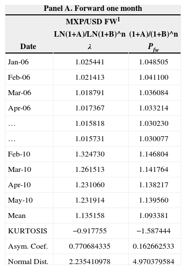
However, when doing a simple inspection of the relationship given in equation (12) it follows a likely problem of non-normality assumption of the original data extracted from the money market. To eliminate this problem, the relationship between the fees is referred back to its natural logarithm, which leads us to modify the equation (12) by a set of P_fw indicator we call λ_i, which can be represented by the following expression:

We note that both P_fw as λ_i capture the so-called International Fisher Effect, λ_i adjusting it, a priori, to be less dispersed. In a preliminary trial, as expected, the addition of the logarithmic function to equation (13) allows the data grouped a behavior close to normal (see table 4). Normality tests were done on the Fw exchange rate to a one-month period and for a 3 month Fw. Parity analyzed in the table was for mexican peso/U.S. Dollar. The rate for the mexican market was the 28-day and 91-day CETE, while for the U.S. market, we considered treasury bills with a one-month and three-month maturity.

Table 4.

Normality Test on the spread in interest rate

Panel A. Forward one month
MXP/USD FW^1
	LN(1+A)/LN(1+B)^n	(1+A)/(1+B)^n
Date	λ	Pfw
Jan-06	1.025441	1.048505
Feb-06	1.021413	1.041100
Mar-06	1.018791	1.036084
Apr-06	1.017367	1.033214
…	1.015818	1.030230
…	1.015731	1.030077
Feb-10	1.324730	1.146804
Mar-10	1.261513	1.141764
Apr-10	1.231060	1.138217
May-10	1.231914	1.139560
Mean	1.135158	1.093381
KURTOSIS	−0.917755	−1.587444
Asym. Coef.	0.770684335	0.162662533
Normal Dist.	2.235410978	4.970379584

Panel B. Forward three months
MXP/USD FW^1
	LN(1+A)/LN(1+B)^n	(1+A)/(1+B)^n
Date	λ	Pfw
Jan-06	1.067897	1.132515
Feb-06	1.060208	1.117890
Mar-06	1.056606	1.110843
Apr-06	1.049728	1.096666
…	1.047138	1.092212
…	1.048036	1.094867
Feb-10	2.018797	1.502704
Mar-10	1.875191	1.487485
Apr 10	1.846749	1.483609
May-10	1.848171	1.485585
Mean	1.439967	1.311504
KURTOSIS	0.376142	−1.491645
Asym. Coef.	1.1009714	0.211805526
Normal Dist.	0.576482512	1.356961397

The analysis of panel A in table 4, on the exchange rate at one month, shows that both curves are asymmetrically positive. Also, equation (13) generates a kurtosis closer to 0 in comparison to the equation (12) which means a more symmetrical distribution. This is ratified by the normal distribution index that shows greater symmetry (2.23541) in equation (13) in contrast to the biased distribution from equation (12). These results suggest the use of equation (13) can be more efficient and capture the differential in interest rate between countries.

In what follows we will identify, precisely, the change in the behavior of unadjusted spreads, consequence of a steady behavior.⁹ The data confirms the superiority of λ against P_fw in that it fosters a greater degree of normalcy. A kurtosis (0.3761 versus −1.4916) closest to 0 and a normal distribution coefficient (0.5764 versus 1.3569) more in line with a symmetrical curve adjustments show that the logarithms of the differences in types are needed to work with less biased values.

Taking a look at the traditional equation (4), we understand that it is subject to the spot rate but also to the behavior of interest rates in an open economy adjusted statistically by a logarithmic function; however, we note the absence of a permanent measure and unexpected volatility of exchange rates.¹⁰ Since Aliber (1973) introduced the concept of portfolio investment to explain the behavior of exchange rates, attention has been focused on quantifying the errors of estimation and market risk as factors that will increase the precision models to predict exchange rates.

There have been several attempts to correctly estimate the level of risk without a strong advance in the field. For example, Brealey et al. (2005) tell us the wisdom to define low risk premium; while for 1996, U.S. Treasury bills were the appropriate proxy for all market risk premiums, however, some time later, they themselves acknowledged that “we have no official position on the market risk premium, but we believe that a range between 6% and 8.5% is reasonable for the United States”.

In 2005, they changed their minds and accepted that the interval should be “between 5 and 8%.” It was such distrust among the policymakers' opinions that Brealey et al. (2005: 154) argue: “This debate comes to just a firm conclusion: do not trust anyone who claims to know what return investors expect”.

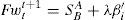
Inclusion of the risk premium under the CAPM approach

As long as we focus cornerstone in the development of our predictive equation seems no more than a chimera, then, our company is impossible. However, we must accept that there are also important and significant advances in the design of the risk premium. In our case we say that the inclusion of the risk premium in the function of the forward exchange rate can be denoted by β_i.

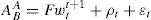
From equation (9) we felt the need to incorporate a risk premium or premium assumed by investors in the exchange rate so the inclusion of β_i as a risk measure is reasonably necessary because it permits to measure the ability of countries to comply with their obligations under delays, which, invariably, will be reflected in the cost of money. If the risk premium of a country decreases, we would expect a drop in interest rates as a significant increase in growth. Then, this risk premium would affect the relationship in the adjusted interest rate and the spot rate as follows:

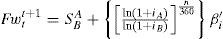
The reduced form of the forward exchange rate would be expressed as:

To shape our risk premium proxy (β′i), a CAPM approach methodology has been used.

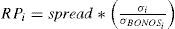
Adjustments to the CAPM approach

To adjust the CAPM approach according to the particularities of the FOREX market we will follow some recommendations: a) García (2009), with respect to the adjustments, these would be made to the variables that make up the initial proposal of the CAPM, b) Damodaran (2002), in relation to an extended CAPM, and c) Madura (2004), who analyzes the additional risk in this approach and that investors incorporate in their expectations. Thus, equation (15) under the proposed Damodaran (2002) is extended to incorporate an underlying risk that is calculated from a spread between sovereign bonds and the relative standard deviation, RP_i, that is:

By adding this underlying risk we would be solving the problem caused by the methods of risk measurement which only added risk to the country risk discount rate (bond spread). The assumption made by Damodaran (2002) is fundamental because it is, correctly, assumed that the whole country risk is not “non-diversifiable”. Damodaran's proposal to measure the country risk (RPi) incorporates the relative standard deviation as follows:

Where:

• σ_BONOSi: The standard deviation of the sovereign bonds for the United States.

• σ_i: Standard deviation of sovereign bonds for country i

• spread: The difference between sovereign bonds.

As proposed by Damodaran, the spread of sovereign bonds would be a useful indicator to approximate quantification of country risk, but, not enough. The spread between interest rates on sovereign bonds is a biased indicator due to investment policies and it is not adjusted for investment decisions of participants. We, therefore, propose a more specific proxy that will redefine the spread according to the proposal made in equation (13) since they correspond directly to the expectations set by investors, but in this case:

• i_A: The risk-free rate of country A's currency

• i_B: The risk-free rate of country B's currency

• n: Term which corresponds both exchange rate and deposit rates fw i

Then, substituting the spread for ρ_i in equation (17) we have:

With respect to the adjustments that are made to other variables in the CAPM, we propose the following:

• R_f: Given that this is the risk free rate, it adapts to the risk-free rate of the base currency, A rate.

• β_i: The variable that measures market risk. We use the proxy EMBI⁺ because it corresponds to a more representative measure of risk for weak markets, as it is the relationship of the mexican peso against other currencies. Also, the substitution of the classical β_i can also be due to the favorable results obtained from the empirical test for the EMBI+¹¹ (see figure A).

  
  

  Figure A.

  Correlation between Mexican Price Index (IPyC) and country risk (EMBI)

  Source: Ponce (2007)

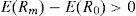
E(R_m) − R_f Since our intention is to find the excess market, we use the method of moving averages to twelve months on the deposit rate to capture this variable. This is consistent because it assumes that investors prefer to shape their minimum performance expectations from historical behavior of the local risk-free rate (country A).

Remember that β′i is the proxy of the risk premium is added/subtracted from the spot rate and that this risk has been formed from an approach adapted from the CAPM. However, in our attempt to refine the risk variable, we should observe the following restrictions:

• 1.

  The elements of the risk premium are divided by 100 to give them a marginal approach,

• 2.

  The risk premium β′i is calculated additive but not a residual, so that market variables join the unit.

• 3.

  Fac_EMBI⁺ is used, which comes from dividing the EMBI⁺/1,000. This approach provides a factor which is interpreted directly as the percentage that the investor in country “A” would have in terms of the situation in the United States.

Then, β′i is composed as follows:

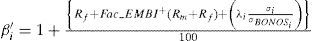
And redefining the equation in terms of ρi, the risk premium can be expressed as:

Empirical model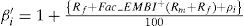

We will prove whether or not the model proposed here can predict prices of financial assets. To demonstrate the degree of precision, we focus on the behavior of random errors that explain the difference between the forecast Fwtt+1 and the exchange rate term ABA.

Our data includes mexican peso (MXP) against the U.S. dollar (USD); the MXP against the pound sterling (GBP) and the MXP against the euro (EUR) for a period that goes from one month to three months. The data spans from January 2006 to May 2010, which is collected from Bloomberg. The interest rates comes from the central banks of the involved countries. The rates used are: for MXP, the 28 and 91-day CETE, for the dollar, treasury bills at one and three months, for the pound, the one-month LIBOR and three-month GBP, and finally for the EUR, the one-month EURIBOR rate to three months is considered. Moreover, the long-term bonds can be appropriate for the dollar Treasury Bonds; for the case of GBP, the British GS to 20 years, and for the EUR Bonds, European government. Furthermore, the EMBI⁺ indicator is also considered and taken from JP Morgan Chase.

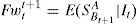
Estimation errors

A test is necessary to measure the degree of success of the function (14) through a practical assessment test which measures the accuracy of forward simulation calculated against the exchange rate at maturity, i.e.,

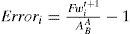
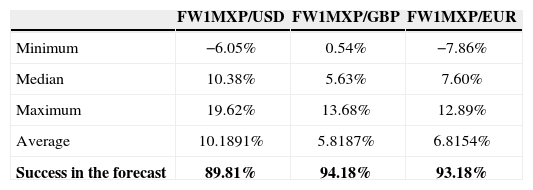
Figure B gives the behavior of the estimation errors found for forward exchange rates to a month. Thus, for the MXP against USD, we have a minimum error forecast rate of −6.05%, which means an overvaluation with respect to the exchange rate at maturity. Moreover, as long as time goes further the error hits 19.62% which means that the formula underestimates the exchange rate. Also, MXP/GBP suffers a greater volatility than the previous interim parity. We note that the handicap is set at 14% and, in general, we also note that we never overvalued the peso against the pound over time. However, for the case of the exchange rate MXP/Eur, we noticed that at a certain point, the formula recognizes a full appreciation of 7.86 and a maximum underestimation around 12.89%.

Figure B.

Error Prediction over time

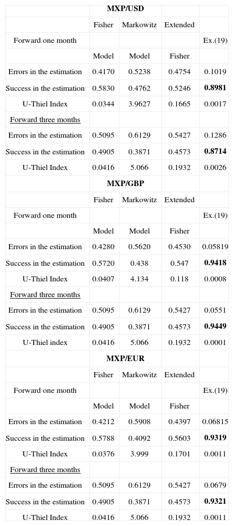
Table 5 shows the relative values of the prediction error for the peso/currency forward within a month. Although significant levels warn volatility in the exchange rate behavior, note that the predictive model (14) succeeds, much higher than other models based only on interest rates. The tests were made on random errors and they show a predictive ability to forecast 89.81% for a month on the MXP/USD, a 94.18% for the rate MXP/GBP and a 93.18% of the MXP against the Euro.

Table 5.

Estimation of forecasting error

	FW1MXP/USD	FW1MXP/GBP	FW1MXP/EUR
Minimum	−6.05%	0.54%	−7.86%
Median	10.38%	5.63%	7.60%
Maximum	19.62%	13.68%	12.89%
Average	10.1891%	5.8187%	6.8154%
Success in the forecast	89.81%	94.18%	93.18%

Period: Jan/2006–May 2010

Forecast success in the predictor

The results shown by equation (14) suggest a very good level of accuracy for the years under assessment (close to or above 90% of accuracy). Contrary to the findings of Bekaert and Hodrick (1993) in the sense that, for them, the premium does not depend on the conditional variance of forecast error, this is included, successfully, in equation 14.

Table 6 shows the accuracy of the classic formulas studied in this paper to forecast the forward exchange rate of the peso against the dollar. The results suggest, again, to be less predictive in classical models compared to equation (14). Much of this predictive failure can be explained by the lack of a risk premium which equation (18) does contain. While the wisdom of the classical formula is around 52%, equation (14) is located at 89; so does the three-month prognosis of being an average accuracy level of 44% in classical equations compared to 87% of the model (14). In the case of forecasts for the pound sterling and the euro, the precision of equation (14) increases at a level above 90% vs. 50% obtained by the classic formulas. How reliable are these results? To this purpose, we apply a validation model that allows us to obtain objective results. Such is the case of U-Thiel index whose results are displayed in table 6 and show that in all the predictions of equation (14) it produces consistent results and investors make rational decisions as our predictors have a better predictive performance than random walk since the index is less than 1.

Table 6.

Validation of predictive models

	MXP/USD
	Fisher	Markowitz	Extended
Forward one month				Ex.(19)
	Model	Model	Fisher
Errors in the estimation	0.4170	0.5238	0.4754	0.1019
Success in the estimation	0.5830	0.4762	0.5246	0.8981
U-Thiel Index	0.0344	3.9627	0.1665	0.0017
Forward three months
Errors in the estimation	0.5095	0.6129	0.5427	0.1286
Success in the estimation	0.4905	0.3871	0.4573	0.8714
U-Thiel Index	0.0416	5.066	0.1932	0.0026
	MXP/GBP
	Fisher	Markowitz	Extended
Forward one month				Ex.(19)
	Model	Model	Fisher
Errors in the estimation	0.4280	0.5620	0.4530	0.05819
Success in the estimation	0.5720	0.438	0.547	0.9418
U-Thiel Index	0.0407	4.134	0.118	0.0008
Forward three months
Errors in the estimation	0.5095	0.6129	0.5427	0.0551
Success in the estimation	0.4905	0.3871	0.4573	0.9449
U-Thiel index	0.0416	5.066	0.1932	0.0001
	MXP/EUR
	Fisher	Markowitz	Extended
Forward one month				Ex.(19)
	Model	Model	Fisher
Errors in the estimation	0.4212	0.5908	0.4397	0.06815
Success in the estimation	0.5788	0.4092	0.5603	0.9319
U-Thiel Index	0.0376	3.999	0.1701	0.0011
Forward three months
Errors in the estimation	0.5095	0.6129	0.5427	0.0679
Success in the estimation	0.4905	0.3871	0.4573	0.9321
U-Thiel Index	0.0416	5.066	0.1932	0.0011

Correctly predict the prognosis of adjusting the risk premium

Despite the progress shown on the robustness of equation (14) the presence of a marginal risk is still possible. Note the high “peaks” that estimation errors reach: from 12.89% and 19.62%. These findings, however, give us the opportunity to continue refining our proposal, which basically seeks to have a greater degree of modeling and control of random errors. In this sense, Mosqueda (2008) finds that the earning power theory is an approach that would help to explain the random behavior of the variables that make up the prospective model. Indeed, this theory establishes the relationship between profit and capital resources to generate and promote profits. Here, the formation of expectations rests on historical data which is estimated from past information enough to predict future events. In this sense, equation (14) would follow from the modeling of a risk premium set given its historical performance:

We show the results on the forward exchange rate calculated by the adjusted risk premium (see table 7). In all cases risk premium was overstated. At a confidence level of 95%, the regression on the possibility of reward (15) in a one-month forward, suggests an adjustment to the risk premium −0.00074, −0.0006 and −0.0019 for the USD, GBP and the EUR respectively. In this case the forecast of the peso against the euro demanded a greater degree of adjustment.

Table 7.

Predictive ability of adjusted risk premium

		MXP/USD	MXP/GBP	MXP/EUR	R2	Adjusted R2
Fw1	No risk premium adjustment	0.89810	0.94180	0.93190	0.9031	0.8991
	Typical error	0.39544	0.61315	0.61944
	Risk premium adjustment	0.89884	0.9424	0.9338
	Typical error	0.33844	0.44359	0.47263
	Adjustment on the risk premium	−0.00074	−0.0006	0.47263
Fw3	No risk premium adjustment	0.8714	0.9449	0.9321	0.9370	0.9276
	Risk premium adjustment	0.9061	0.9507	0.9553
	Typical error	0.38635	0.40098	0.40837
	Adjustment on the risk premium	−0.0347	−0.0058	−0.0232

FW1: Forward rate of one month

FW1: Forward rate of one month FW3: Forward rate of three months

Also, the regression on the adjusted premium is observed in a multiple correlation coefficient that is very high: a R² of 0.9031 and an adjusted R² of 0.8991, which correspond to the typical error levels as low. With respect to three-month forward, it also recognizes the need for a greater degree of adjustment on the risk premium because the behavior of the estimation errors may become, mostly, a volatile and erratic behavior over time. Thus, same way as in the calculation of the one-month exchange rate, the results suggest a correction to the risk premium, given a confidence level of 95%, from −0.0347, −0.0058 and −0.0232, respectively.

The increase in the coefficient of determination (R² and R² Adj. of 0.9370 and 0.9275 compared with 0.9031 R² and adjusted R² of 0.8991 obtained with equation (14) without adjusting for risk) is interpreted as an increase in the ability of β′1 to collect the investor's expectations and to discount the value of the spot rate.

In previous studies, Mark (1995), for example, found multiple correlation coefficients with levels ranging from 0.179 (for the Canadian market) up to 0771 (for the Swiss franc), without coefficients statistically significant. On the other side, Neely and Sarno (2002), incorporated the value at risk approach, replicating the study of Mark (1995) with coefficients of determination similar to Mark's: 0,065 for the Canadian dollar, 0.0675 to the German mark disappeared, 0,173 for the yen and a 0,137 in the case of the Swiss market.

Based on the above, we can infer that by the adjustment to the risk premium for the possibility of Premium and given a non-seasonal historical behavior, it is possible to achieve a higher degree of predictive ability.

Figure C shows, by way of example, an almost perfect correlation between the marginal behavior of the forward rate, Fwtt+1, estimated by equation (14), with the percentage changes that occur in the spot rate at maturity, ABA. In this sense, it is clear the relevance of incorporating the adjusted risk premium, β′i, because it captures, as suggested by Harvey (1991), the performance variant of the premium demanded by investors across different contexts and times.

Figure C.

Monthly Variation in the Exchange rate MXP/USD for a month

Source: Bloomberg and Central Banks

Conclusions

In light of these findings we can conclude that the results are encouraging because they not only model the behavior of the risk premium but the function given in equation (14) has a dynamic characteristic that makes it more powerful. Note, for example, that the high degree of accuracy and specification permits to reinforce the idea that interest rates can be an unbiased proxy for the exchange rate subject to adjustment under the CAPM approach.

We noticed a close and strong correlation between changes in spot rates and forward estimates for equation (14) that allows us to infer that it is possible to keep accurate prices with consistent forecast regarding the terms. The spot exchange rate itself is an unbiased proxy for forward exchange rates when it is adjusted to the expectations that are formed by investors. The latter goes along the line of Jensen (1978) who already establishes the need for a prime to offset risk.

Despite the findings of other studies, we found no random relationship in the appropriate level of risk that investors expect, but on the contrary, we see some rationality in shaping expectations of risk that would occur from the different adjusted economic positions of countries. The results provided by economic models, mainly those based on interest rates, are better specified than those obtained in a study of random walk.