


In this paper, we compute the implied equity duration (IED) for the non-financial companies listed in the Spanish stock market for the first time, to the best of our knowledge. This measure of risk adapts the traditional expression of the duration of a bond to the stock context. We also conduct a sector analysis and a size analysis using the Ibex indices composition. The results are then compared with those from the U.S. stock market and related to other proxies of equity risk. This analysis shows that there is a significant relation between the IED and the earnings to price ratio, the book to market ratio and the sales growth rate, but not to capitalisation, thus excluding the presence of a size effect. The results support the relation of the IED with the high minus low factor, thereby suggesting that the latter is subsumed in this measure.
The interest rate risk analysis in the fixed income context is built on a rigorous methodological approach based on discounting the cash flows promised by the issuer. The central concept in this framework is the duration, a risk measure commonly accepted and used by both academia and practitioners. This concept, first presented by Macaulay (1938), is defined as the weighted average of the times at which bondholders receive the cash flows from a bond, where the weights are equal to the present values of the payments normalised with respect to the price of the bond. The Macaulay duration effectively measures the sensitivity of a bond to changes in the discount rate in the fixed cash flow model, i.e., the yield to maturity.
However, the interest rate risk analysis for equities does not have a unique framework. Thus, we find from analysis based on simple models of stock valuation (Leibowitz, 1986) to others based on an empirical linear relation between the variations in stock prices and the variations in market interest rates a compromise solution. Despite the efforts of researchers, reaching up prepend the need of results to the rigour of the analysis, none of these methodologies has provided the necessary results to become a reference methodology.
In this context, Dechow et al. (2004) bridge the gap between techniques used in the analyses of bonds and equities, thus developing a measure of implied equity duration (IED) based on the Macaulay duration for a bond. Their methodology also combines, in the equity context, the two aforementioned approaches as they used an analytical model of stock valuation based on the discounted cash flows that matches the market quote by adjusting the terminal cash flow scheme.
Thus, implementing the IED requires estimating in advance the expected cash flows by the equity, in which a two-step process is used. First, using a simple model based on historic financial data, cash flows are estimated for a finite prediction horizon. It is then assumed that the rest of the equity market price is distributed as a perpetual start on the finite prediction horizon. Accordingly, applying the Macaulay duration formula to these cash flows leads to the IED.
Dechow et al. (2004) compute the IED for each of the companies using the available data from the NYSE, AMEX and NASDAQ, between 1963 and 1998, and obtain an IED average of 15.13 years, with a standard deviation of 4.09. The results of their empirical tests show that the IED explains the risk characteristics for the stock returns, resulting in a positive and significant relationship with the volatility of the stock returns and their betas, and that the IED provides more prediction power of these variables than does its own lagged variables. Furthermore, the IED captures a strong common factor in the profitability of the shares that encompass the common factor related to the book-to-market ratio (BtM) whose empirical properties were revealed by Fama and French (1993).
In this context, the objective of this paper is to compute the IED for the listed firms in the Spanish stock market with the data available at the end of 2011, compare the results with those obtained in Dechow et al. (2004) for the U.S. market, perform sector and size analyses and search for the relationship of the IED with other commonly used variables as risk proxies to find evidence of the relationship between the IED and the company growth options as well as the size and effects of the IED as gathered by the Fama and French factors.
The latter analysis links this work within the empirical literature that relates the systematic risk of stock with the premium value by breaking down the betas for assets in cash flow betas and discount-rate betas. In this context, Campbell and Mei (1993) find that the discount-rate betas represent the large part of the total beta of the companies, and based on that, Cornell (1999) suggests that the high betas for growth stocks are a consequence of a greater weight of the cash flows removed in time, or equivalently, of growth stocks longer duration. Campbell et al. (2009) show that the value premium is a consequence of the differences in the timed schedule of the expected cash flows by the shareholder represented by the duration. At the same time, Da (2009) shows how cross-sectional differences in the duration of companies could explain an important part of the stock returns. In summary, as Santa-Clara (2004) has noted, the IED “is an interesting new approach to measuring stock risk”.
This paper is organised as follows. In the next section, we derive the measure of interest rate risk of the equity, the IED. Section 3 describes the data selection process. Section 4 presents the results: (i) the results of computing the IED for each company and the main statistics for the entire sample; (ii) the results of the sectorial and size analyses carried out using the stock market activity classification and size indices; and (iii) the results related to the relationship of the IED with other variables used as risk proxies, which include the earnings-to-price ratio (EPR), the BtM, the sales-growth-rate (SGR) and the capitalisation (CAP). Finally, Section 5 summarises the results and states the main conclusions.
2Implied equity durationMacaulay (1938) first introduced the duration concept as the weighted average of the times until fixed bond cash flows are received. Hicks (1939) further showed that the duration is essentially a measure of the elasticity of bonds to interest rates. From the bond price formula, it is straightforward to note that bond prices are inversely related to their yield to maturity as a unique risk factor.1
However, in the equity valuation, there are many factors, including interest rate, that affect cash flows beyond the discount rate used to compute their present values. Lintner (1971), Boquist et al. (1975) and Livingston (1978) initially proposed the concept of stock duration, and then in the works of Leibowitz (1986) and Leibowitz et al. (1989), it was first computed for individual firms. More recent studies in this line are Cohen (2002), Hamelink et al. (2002)Lewin et al. (2007), Shaffer (2007) and Leibowitz et al. (2010).
In Boquist et al. (1975), the stock duration measure is built on the dividend discount model. However, Leibowitz (1986) used market quotes to develop an alternative measure. But, as Leibowitz and Kogelman (1993) noted, the values for both measures are significantly different, even when the compensation between price risk and reinvestment risk is taken into account as proposed by Johnson (1989). These differences determine the so-called duration paradox and give rise to works, such as Leibowitz and Kogelman (1993) and Hurley and Johnson (1995), that attempt, though unsuccessfully, to conciliate the two measures.
In this paper, we use an alternative stock duration measure proposed by Dechow et al. (2004) that is based on the Macaulay's duration for a bond (one time period before the first future cash flow):
where CFt are the bond cash flows; r is the bond yield to maturity; and P is the actual price of the bond.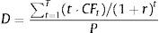
As previously mentioned, the bond duration is a weighted average of the maturities of T-cash flows, where the weights are the relative contribution of each cash flow to the actual bond price. The main role of the bond duration in the fixed income analysis is as a measure of the bond's price sensitivity to changes of bond yield to maturity.
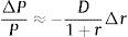
Differentiating the bond price expression with respect to its yield to maturity, we obtain the relationship between changes in the price of a bond and changes in its yield to maturity as a function of the duration:
We can rewrite this relationship and express it in discrete form to obtain the following relation between the relative bond price changes and the discrete changes in its yield to maturity as a function of [D/(1+r)], the so-called modified duration,Extending the duration concept to equities introduces one drawback. That is, while the amount and timing of bond cash flows are usually fixed in advance so the bondholder has little uncertainty, the cash flows of equities are not specified in advance and may be subject to great uncertainty.
If we decompose the duration formula shown in Eq. (1) into two parts, one with a finite horizon up to T and another with an infinite horizon from T, we obtain Eq. (4), which expresses the equity duration as a sum of the weighted values of the duration of the cash flows for the finite horizon and the duration of terminal cash flows.
where P is the market firm capitalisation; CFt are the predicted firm pay outs to the stockholders; and r represents the expected return on firm equity.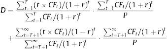
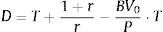
If we also assume that the terminal cash flows are a perpetual with an actual value equal to the difference between the market capitalisation and the present value of the predicted cash flows for the finite period, then:
As the duration of the perpetual that begins in T periods is [T+(1+r)/r], substituting (5) into (4), we obtain the following expression for the IED:To compute Eq. (6), we need predictions of firm cash flows for the finite period (0, T]. In this sense, Dechow et al. (2004) used a cash flows prediction model based on previous results that relate accounting measures with future cash flows (Nissim and Penman, 2001). Thus, from the accounting identity of the flows distributed to shareholders from the firm earnings and their book value, we have the following:where Et is the firm earnings at the end of period t; and BVt represents the firm book value at the end of period t.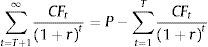


Rewriting the right term of Eq. (7), we obtain:
Thus, a cash flow forecast for period t can be computed with (i) the return on equity (ROE) in period t, i.e., Et/BVt−1; and (ii) the growth rate of equity in period t, i.e., (BVt−BVt−1)/BVt−1.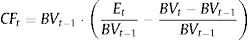
Dechow et al. (2004) modelled ROE as a first-order autoregressive process with an autocorrelation coefficient based on the reversion rate of a mean reversion process of ROE with a mean equal to the historical cost of equity. It is generally accepted that the ROE follows a mean reverting process (Stigler, 1963; Penman, 1991). Further, the economic intuition and the empirical evidence (Nissim and Penman, 2001) suggest that the mean that reverses the ROE approximates the cost of equity.
The results of Nissim and Penman (2001) also show that sales growth rate is the best proxy of the future growth rate of the equity. Accordingly, Dechow et al. (2004) modelled the growth rate of equity as a first-order autoregressive process with an autocorrelation coefficient equal to the reversion rate of the mean reversion process of the sales growth rate and a mean equal to the long-term macroeconomic growth rate.
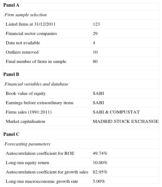
3DataComputing the IED from Eq. (6) requires year-end data on four financial variables and four parameters. The financial variables are the firm book value (both current and lagged one year), the firm sales (both current and lagged one year), the firm earnings (current) and the market firm capitalisation (current). The four parameters are the autocorrelation coefficient for the ROE, the autocorrelation coefficient for sales growth, the cost of equity and the long-term growth rate of the economy.
From the SABI database, we obtain the three accounting variables at the end of year 2011 and 2010. SABI includes the annual accounting statements for Spanish and Portuguese firms. We select the non-financial firms listed on the Spanish stock market, of which there are 90.2 Then, we eliminate the influence of outside atypical values. In our case, this is achieved by removing the 5% extreme values of the sales growth rate, thus reducing the final sample to eighty firms.
From the Madrid Stock Exchange, we obtain the market variable, capitalisation, the sectorial firms classification and the Ibex indices classification. Non-financial firms are grouped into five sectors with their corresponding numbers, as summarised in Table 1, panel D: Oil & Energy; Commodities, Industry and Construction; Consumer Goods; Consumer Services; and Technology and Communications. Most non-financial firms are present on December 31, 2011, in three Ibex indices according to their size: Ibex 35, Ibex Medium Cap and Ibex Small Cap, as summarised in Table 1, panel D.
Summary of firm sample selection, financial variables and parameters used in the estimation of implied equity duration.
| Panel A | |
| Firm sample selection | |
| Listed firms at 31/12/2011 | 123 |
| Financial sector companies | 29 |
| Data not available | 4 |
| Outliers removed | 10 |
| Final number of firms in sample | 80 |
| Panel B | |
| Financial variables and database | |
| Book value of equity | SABI |
| Earnings before extraordinary items | SABI |
| Firms sales (1991:2011) | SABI & COMPUSTAT |
| Market capitalisation | MADRID STOCK EXCHANGE |
| Panel C | |
| Forecasting parameters | |
| Autocorrelation coefficient for ROE | 49.74% |
| Long-run equity return | 10.00% |
| Autocorrelation coefficient for growth sales | 82.95% |
| Long-run macroeconomic growth rate | 5.00% |
| Sectors | # | IBEX35 | IBEX MC | IBEX SC |
| Panel D: summary of sample companies by index and sector | ||||
| Oil & Energy | 8 | 6 | 0 | 1 |
| Commodities | 23 | 8 | 5 | 6 |
| Consumer Goods | 27 | 3 | 5 | 10 |
| Consumer Services | 17 | 3 | 4 | 4 |
| Technology | 5 | 3 | 1 | 0 |
| Totals | 80 | 23 | 15 | 21 |
Data have been obtained from the database for Spanish and Portuguese companies SABI (Bureau Van Dijk Group), from Compustat Global (Standard & Poor's), which includes 145 companies for the Spanish Market that compose 100% of the listed companies, and from the Madrid Stock Exchange (www.bolsamadrid.es). For a long-run growth rate, we used the long-term average for the time series of the GDP, obtained from the Spanish National Statistics Institute (www.ine.es). In Panel D, activity sectors and indices appear according to the Madrid Stock Exchange classifications.
Regarding the parameters, the long-term average cost of equity and the long-term growth rate of the economy are based on long-term historical averages that approximate the parameters to 10% and 5%, respectively, as listed in Table 1, panel C. As in Dechow et al. (2004), we use a constant cross-section forecast of the cost of equity to ensure that each firm's IED differs only by the different distribution of the expected cash flows. Both the ROE autocorrelation coefficient and the sales growth rate autocorrelation coefficient are estimated as the mean of firm values computed using SABI and COMPUSTAT data for sample companies with at least 10 years of available data. Their values, 0.4974 and 0.8295, respectively, as listed in Table 1 – panel C, are applied to all firms as market variables.
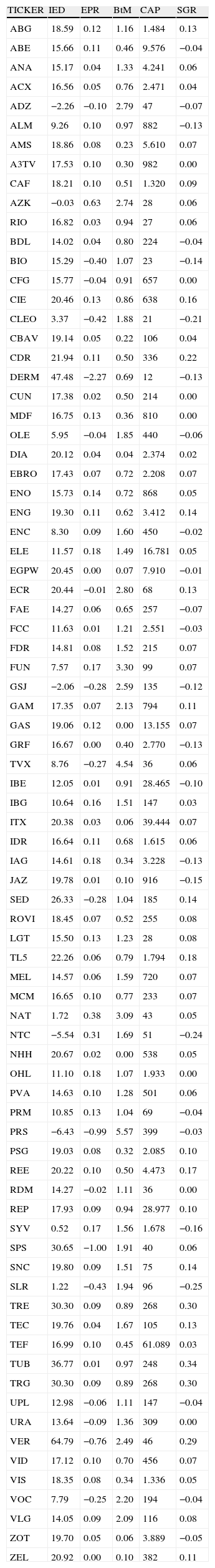
4Results4.1The IED for the sample firmsFor the IED computation thought Eq. (6), we use a finite prediction horizon of 10 years, as in Dechow et al. (2004), after checking that the mean reversion, both for the SGR and the ROE, are completed before this time. Table 2 shows the IED for the sample firms at the end of year 2011. In this table, we also show the others variables that are usually used as risk proxies (EPR, BtM, CAP, SGR) on the same date.
Implied equity duration, earning-to-price ratio, book-to-market, market capitalisation and sales growth rate.
| TICKER | IED | EPR | BtM | CAP | SGR |
| ABG | 18.59 | 0.12 | 1.16 | 1.484 | 0.13 |
| ABE | 15.66 | 0.11 | 0.46 | 9.576 | −0.04 |
| ANA | 15.17 | 0.04 | 1.33 | 4.241 | 0.06 |
| ACX | 16.56 | 0.05 | 0.76 | 2.471 | 0.04 |
| ADZ | −2.26 | −0.10 | 2.79 | 47 | −0.07 |
| ALM | 9.26 | 0.10 | 0.97 | 882 | −0.13 |
| AMS | 18.86 | 0.08 | 0.23 | 5.610 | 0.07 |
| A3TV | 17.53 | 0.10 | 0.30 | 982 | 0.00 |
| CAF | 18.21 | 0.10 | 0.51 | 1.320 | 0.09 |
| AZK | −0.03 | 0.63 | 2.74 | 28 | 0.06 |
| RIO | 16.82 | 0.03 | 0.94 | 27 | 0.06 |
| BDL | 14.02 | 0.04 | 0.80 | 224 | −0.04 |
| BIO | 15.29 | −0.40 | 1.07 | 23 | −0.14 |
| CFG | 15.77 | −0.04 | 0.91 | 657 | 0.00 |
| CIE | 20.46 | 0.13 | 0.86 | 638 | 0.16 |
| CLEO | 3.37 | −0.42 | 1.88 | 21 | −0.21 |
| CBAV | 19.14 | 0.05 | 0.22 | 106 | 0.04 |
| CDR | 21.94 | 0.11 | 0.50 | 336 | 0.22 |
| DERM | 47.48 | −2.27 | 0.69 | 12 | −0.13 |
| CUN | 17.38 | 0.02 | 0.50 | 214 | 0.00 |
| MDF | 16.75 | 0.13 | 0.36 | 810 | 0.00 |
| OLE | 5.95 | −0.04 | 1.85 | 440 | −0.06 |
| DIA | 20.12 | 0.04 | 0.04 | 2.374 | 0.02 |
| EBRO | 17.43 | 0.07 | 0.72 | 2.208 | 0.07 |
| ENO | 15.73 | 0.14 | 0.72 | 868 | 0.05 |
| ENG | 19.30 | 0.11 | 0.62 | 3.412 | 0.14 |
| ENC | 8.30 | 0.09 | 1.60 | 450 | −0.02 |
| ELE | 11.57 | 0.18 | 1.49 | 16.781 | 0.05 |
| EGPW | 20.45 | 0.00 | 0.07 | 7.910 | −0.01 |
| ECR | 20.44 | −0.01 | 2.80 | 68 | 0.13 |
| FAE | 14.27 | 0.06 | 0.65 | 257 | −0.07 |
| FCC | 11.63 | 0.01 | 1.21 | 2.551 | −0.03 |
| FDR | 14.81 | 0.08 | 1.52 | 215 | 0.07 |
| FUN | 7.57 | 0.17 | 3.30 | 99 | 0.07 |
| GSJ | −2.06 | −0.28 | 2.59 | 135 | −0.12 |
| GAM | 17.35 | 0.07 | 2.13 | 794 | 0.11 |
| GAS | 19.06 | 0.12 | 0.00 | 13.155 | 0.07 |
| GRF | 16.67 | 0.00 | 0.40 | 2.770 | −0.13 |
| TVX | 8.76 | −0.27 | 4.54 | 36 | 0.06 |
| IBE | 12.05 | 0.01 | 0.91 | 28.465 | −0.10 |
| IBG | 10.64 | 0.16 | 1.51 | 147 | 0.03 |
| ITX | 20.38 | 0.03 | 0.06 | 39.444 | 0.07 |
| IDR | 16.64 | 0.11 | 0.68 | 1.615 | 0.06 |
| IAG | 14.61 | 0.18 | 0.34 | 3.228 | −0.13 |
| JAZ | 19.78 | 0.01 | 0.10 | 916 | −0.15 |
| SED | 26.33 | −0.28 | 1.04 | 185 | 0.14 |
| ROVI | 18.45 | 0.07 | 0.52 | 255 | 0.08 |
| LGT | 15.50 | 0.13 | 1.23 | 28 | 0.08 |
| TL5 | 22.26 | 0.06 | 0.79 | 1.794 | 0.18 |
| MEL | 14.57 | 0.06 | 1.59 | 720 | 0.07 |
| MCM | 16.65 | 0.10 | 0.77 | 233 | 0.07 |
| NAT | 1.72 | 0.38 | 3.09 | 43 | 0.05 |
| NTC | −5.54 | 0.31 | 1.69 | 51 | −0.24 |
| NHH | 20.67 | 0.02 | 0.00 | 538 | 0.05 |
| OHL | 11.10 | 0.18 | 1.07 | 1.933 | 0.00 |
| PVA | 14.63 | 0.10 | 1.28 | 501 | 0.06 |
| PRM | 10.85 | 0.13 | 1.04 | 69 | −0.04 |
| PRS | −6.43 | −0.99 | 5.57 | 399 | −0.03 |
| PSG | 19.03 | 0.08 | 0.32 | 2.085 | 0.10 |
| REE | 20.22 | 0.10 | 0.50 | 4.473 | 0.17 |
| RDM | 14.27 | −0.02 | 1.11 | 36 | 0.00 |
| REP | 17.93 | 0.09 | 0.94 | 28.977 | 0.10 |
| SYV | 0.52 | 0.17 | 1.56 | 1.678 | −0.16 |
| SPS | 30.65 | −1.00 | 1.91 | 40 | 0.06 |
| SNC | 19.80 | 0.09 | 1.51 | 75 | 0.14 |
| SLR | 1.22 | −0.43 | 1.94 | 96 | −0.25 |
| TRE | 30.30 | 0.09 | 0.89 | 268 | 0.30 |
| TEC | 19.76 | 0.04 | 1.67 | 105 | 0.13 |
| TEF | 16.99 | 0.10 | 0.45 | 61.089 | 0.03 |
| TUB | 36.77 | 0.01 | 0.97 | 248 | 0.34 |
| TRG | 30.30 | 0.09 | 0.89 | 268 | 0.30 |
| UPL | 12.98 | −0.06 | 1.11 | 147 | −0.04 |
| URA | 13.64 | −0.09 | 1.36 | 309 | 0.00 |
| VER | 64.79 | −0.76 | 2.49 | 46 | 0.29 |
| VID | 17.12 | 0.10 | 0.70 | 456 | 0.07 |
| VIS | 18.35 | 0.08 | 0.34 | 1.336 | 0.05 |
| VOC | 7.79 | −0.25 | 2.20 | 194 | −0.04 |
| VLG | 14.05 | 0.09 | 2.09 | 116 | 0.08 |
| ZOT | 19.70 | 0.05 | 0.06 | 3.889 | −0.05 |
| ZEL | 20.92 | 0.00 | 0.10 | 382 | 0.11 |
For each firm, this table shows: IED at year-end 2011; 2011 year-end earning-to-price ratio as annual earnings over market capitalisation; BtM: book-to-market ratio calculated as year-end 2011 book value of equity over market capitalisation; market capitalisation at year-end 2011 in millions of euros; and sales growth rate as sales annual difference over the previous period sales [(Salest−Salest−1)/Salest−1].
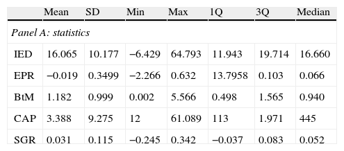
In Table 3, panel A, we summarise the main statistics for all these variables. The average for the IED is 16.07 years with a standard deviation of 10.18 years. The value that defines the lowest quartile is 11.94, while the value that defines the superior quartile is 19.71. Thus, for most firms, the IED is below 21 years, the IED corresponding to terminal cash flows. Therefore, for these firms, only a small portion of the time distribution of their actual value is explained by discounted cash flows for the 10-year finite period. The minimum value of the IED is −6.43 years,3 and the maximum value is 64.79 years. In Table 3, panel B, we show correlations between all the variables included in the analysis. The correlations between the IED and the other variables are generally related to intensity and the expected signs.
Descriptive statistics for implied equity duration and other related measures.
| Mean | SD | Min | Max | 1Q | 3Q | Median | |
| Panel A: statistics | |||||||
| IED | 16.065 | 10.177 | −6.429 | 64.793 | 11.943 | 19.714 | 16.660 |
| EPR | −0.019 | 0.3499 | −2.266 | 0.632 | 13.7958 | 0.103 | 0.066 |
| BtM | 1.182 | 0.999 | 0.002 | 5.566 | 0.498 | 1.565 | 0.940 |
| CAP | 3.388 | 9.275 | 12 | 61.089 | 113 | 1.971 | 445 |
| SGR | 0.031 | 0.115 | −0.245 | 0.342 | −0.037 | 0.083 | 0.052 |
| IED | EPR | BtM | CAP | SGR | |
| Panel B: correlations (Pearson/Spearman) | |||||
| IED | – | −0.122 | −0.564 | 0.192 | 0.621 |
| EPR | −0.365 | – | −0.144 | 0.283 | 0.212 |
| BtM | −0.393 | −0.231 | – | −0.576 | −0.038 |
| CAP | 0.027 | −0.218 | 0.098 | – | 0.046 |
| SGR | 0.587 | −0.051 | 0.180 | −0.004 | – |
Pearson linear correlation coefficients appear in Panel B below the diagonal and Spearman linear correlation coefficients are above the diagonal. IED: implied equity duration at year-end 2011; EPR: 2011 year-end earning-to-price ratio as annual earnings over market capitalisation; BtM: book-to-market ratio calculated as year-end 2011 book value of equity over market capitalisation; CAP: market capitalisation at year-end 2011 in millions of euros; and SGR: sales growth rate as sales annual difference over the previous period sales [(Salest−Salest−1)/Salest−1].
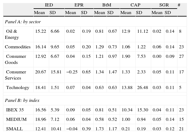
To deepen the characterisation of the sample firms through their IEDs, we conduct a sectorial analysis that groups firms by activity and an analysis by Ibex indices that classifies firms by size. These analyses allow us to perceive evidence of potential firm growth options and size effects. For this, all firms are grouped into five sectors (similar to the Madrid Stock Exchange), and alternatively, into three groups depending on the Ibex index to which each firm belongs, if any.
Table 4 shows the main statistics by firm groups of the variables involved in the analysis. By sectors, in panel A, we note that both the IED averages and their standard deviations vary considerably among sectors, in line with the other variables. The Consumer Goods sector has the minimum sectorial IED average at 12.92 years, while the Consumer Services sector has the maximum sectorial IED average at 20.67 years. However, we do not sense from these statistics a clear relation between the IED and any other variable.
Descriptive statistics for measures by sector and index.
| IED | EPR | BtM | CAP | SGR | # | ||||||
| Mean | SD | Mean | SD | Mean | SD | Mean | SD | Mean | SD | ||
| Panel A: by sector | |||||||||||
| Oil & Energy | 15.22 | 6.66 | 0.02 | 0.19 | 0.81 | 0.67 | 12.9 | 11.12 | 0.02 | 0.14 | 8 |
| Commodities | 16.14 | 9.65 | 0.05 | 0.20 | 1.29 | 0.73 | 1.06 | 1.22 | 0.06 | 0.14 | 23 |
| Consumer Goods | 12.92 | 6.67 | 0.04 | 0.15 | 1.21 | 0.97 | 1.90 | 7.53 | 0.00 | 0.09 | 27 |
| Consumer Services | 20.67 | 15.81 | −0.25 | 0.65 | 1.34 | 1.47 | 1.33 | 2.33 | 0.05 | 0.11 | 17 |
| Technology | 18.41 | 1.51 | 0.07 | 0.04 | 0.63 | 0.63 | 13.88 | 26.48 | 0.03 | 0.11 | 5 |
| Panel B: by index | |||||||||||
| IBEX 35 | 16.56 | 5.39 | 0.09 | 0.05 | 0.81 | 0.51 | 10.34 | 15.30 | 0.04 | 0.11 | 23 |
| MEDIUM | 18.96 | 7.12 | 0.06 | 0.04 | 0.58 | 0.52 | 1.00 | 0.94 | 0.05 | 0.14 | 15 |
| SMALL | 12.41 | 10.41 | −0.04 | 0.39 | 1.73 | 1.17 | 0.21 | 0.19 | 0.03 | 0.12 | 21 |
Means and standard deviations for each measure by sectors according Madrid Stock Exchange classification in panel A and by Ibex index in panel B (Ibex 35, Ibex Medium Cap and Ibex Small Cap). IED: implied equity duration at year-end 2011; EPR: 2011 year-end earning-to-price ratio as annual earnings over market capitalisation; BtM: book-to-market ratio calculated as year-end 2011 book value of equity over market capitalisation; CAP: market capitalisation at year-end 2011 in millions of euros; and SGR: sales growth rate as sales annual difference over the previous period sales [(Salest−Salest−1)/Salest−1].
The index grouping, in panel B, shows that the average IED variability and the standard deviations are less than that of other variables. Moreover, no relation between the IED and size is found. However, a relation between the IED and the BtM and a relation between the IED and the SGR appear when we group firms by size.
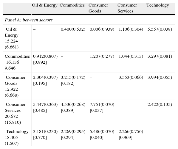
In Table 5, we report the results of different means tests between sectors in panel A and between indices in panel B. We report results for both parametric and non-parametric tests, given the small number of observations included in any of the groups.4
Tests of IED means difference and equal variances among groups.
| Oil & Energy | Commodities | Consumer Goods | Consumer Services | Technology | |
| Panel A: between sectors | |||||
| Oil & Energy15.224(6.661) | – | 0.400(0.532) | 0.006(0.939) | 1.106(0.304) | 5.557(0.038) |
| Commodities16.1369.646 | 0.912(0.807)[0.892] | – | 1.207(0.277) | 1.044(0.313) | 3.297(0.081) |
| Consumer Goods12.922(6.668) | 2.304(0.397)[0.195] | 3.215(0.172)[0.182] | – | 3.553(0.066) | 3.994(0.055) |
| Consumer Services20.672(15.810) | 5.447(0.363)[0.485] | 4.536(0.268)[0.389] | 7.751(0.070)[0.037] | – | 2.422(0.135) |
| Technology18.405(1.507) | 3.181(0.230)[0.770] | 2.269(0.295)[0.294] | 5.486(0.070)[0.040] | 2.266(0.756)[0.969] | – |
| IBEX35 | Medium | Small | |
| Panel B: between size index groups | |||
| IBEX3516.789(4.811) | – | 0.526(0.473) | 9.899(0.003) |
| Medium18.951(7.128) | 2.402(0.245)0.269 | – | 3.677(0.064) |
| Small13.160(15.840) | 4.144(0.113)[0.226] | 6.546(0.032)[0.096] | – |
The first column of the table shows the means and standard deviations for the sectors and indices firm groups. In the body of the table, we have collected below the diagonal the mean difference by sectors and indices, respectively, followed by the parametric significance level for the t-statistic in parentheses and asymptotic significance for non-parametric tests in brackets (Mann–Whitney U if one assumes normality and Wilcoxon W otherwise). Above the diagonal we show the results of the Levene test for equality of variances followed by significance in parentheses that determines the test of means difference to use.
When we analyse the mean differences between sectors, we find two significant differences. In this sense, the parametric and the non-parametric tests have shown very similar results. We note that the mean difference of approximately 7.75 years between the Consumer Goods sector, which has the lowest IED, and the Consumer Services sector, which has the highest sectorial IED, is significant at 10% in the parametric test and at 5% in the non-parametric test. We find an identical result for the mean difference of approximately 6.48 years between the Consumer Goods sector and the Technology and Communications sector, the second largest sectorial IED. These results confirm the relation between the IED and the firm growth options, and they strengthen the relationship between the IED and the BtM.
With respect to the mean differences between the various indices listed in panel B of Table 5, in only one case do we observe significant results, that is, the means difference between the IbexMediumCap index group and IbexSmallCap index group, with a significance level of 5% in the parametric test and a 10% significance level in the non-parametric test. Namely, no significant results for the means difference between index Ibex35 and index IbexSmallCap are found. These results support the argument that the IED does not reflect a size effect, i.e., there is not a relationship between the firm's IED and its size (CAP).
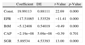
4.3Cross-sectional regression analysisGiven that the relationship between the IED and the EPR and between the IED and the BtM has been analytically proven by Dechow et al. (2004), as reflected in Appendix A, and given the previous results that (i) confirm empirically these relations in the sample data, (ii) show a relation between the IED and SGR, and (iii) show the usefulness of the size to clarify some of these relationships, we perform a cross-sectional regression analysis between the IED and the EPR, the BtM and the SGR, using CAP as a control variable.5
In Table 6, we report the results. As expected, the significance of the EPR and BtM in explaining the IED is clear. The SGR also shows significant explanatory power of the IED as expected due to its important role in forecast firms cash flows. However, the market capitalisation variable has not shown significant results. This is likely because the BtM withdraws its effect, as noted by Chen (2011).
IED cross-sectional regression against the other corporate risk proxies.
| Coefficient | DE | t-Value | p-Value | |
| Const. | 19.99113 | 0.88111 | 22.69 | 0.000 |
| EPR | −17.51065 | 1.53529 | −11.41 | 0.000 |
| BtM | −5.12408 | 0.54019 | −9.49 | 0.000 |
| CAP | −2.19e−08 | 5.69e−08 | −0.39 | 0.701 |
| SGR | 5.89534 | 4.53393 | 13.00 | 0.000 |
The coefficients in the table are estimated by linear regression through the equation:

Following is the standard deviation of the t-statistic coefficient and its significance. The F statistic obtained for four degrees of freedom was 79.17, the R-squared of 80.85% and adjusted R-squared of 79.83%. IED: implied equity duration at year-end 2011; EPR: 2011 year-end earning-to-price ratio as annual earnings over market capitalisation; BtM: book-to-market ratio calculated as year-end 2011 book value of equity over market capitalisation; CAP: market capitalisation at year-end 2011 in millions of euros; and SGR: sales growth rate as sales annual difference over the previous period sales [(Salest−Salest−1)/Salest−1].
In this paper, we compute for the first time, to the best of our knowledge, the implied duration of equity (IED) for the non-financial listed firms on the Spanish Stock Market, as developed in Dechow et al. (2004). Concretely, the IED is computed for December 31, 2011, for eighty firms. The results are consistent with those presented in Dechow et al. (2004), although the Spanish IED is slightly higher due to the different expected return on equity used in each context.
A further sector and size index analysis enables us to test mean differences between firm groups. The tests implemented across sectors confirm the existence of significant differences between the sectors with the most extreme IED suggesting a relation between IED and firm growth options. The tests for the mean differences between Ibex indices showed that they are, in some cases, significant but without a correlation between firm size and firm IED.
The correlations between the IED and the usual ratios that describe company risk, EPR and BtM are of the expected signs and intensity. A further regression analysis, adding market capitalisation and sales growth rate, confirms the ability of these ratios and sales growth rate to explain the IED. In contrast, capitalisation is not significant, thus removing any possibility of a size effect.
A remarkable result is that the relationship present in the valuation models between the IED and the traditional indicator for value (growth), the BtM, can also be found in the analysed data such that the smaller the BtM, the longer the mean maturity of firm cash flows, and vice versa. This result is consistent with previous results, thus suggesting that the BtM factor from Fama and French could be a simple approximation to a more fundamental cash flow risk factor captured by stock duration in which, according to the results shown herein, it also collects information on the EPR and Sales Growth Rate.
The authors thank comments from the editor, Francisco González, and an anonymous referee of the Spanish Review of Financial Economics, from Juan Nave, and from participants in the XVI Applied Economics Meeting (Granada, 2013), and in the internal seminars at Universidad de Castilla – La Mancha, Universidad de Murcia, Universidad de Valencia, Universidad de Huelva and Universidad CEU Cardenal Herrera. They also thank financial support from Gobierno de España (MICINN ECO2009-13616 and MEYC ECO2012-36685) and from Banco Santander (Copernicus UCH-CEU 36/12).
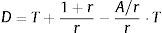
Dechow et al. (2004) showed the analytical links between IED and EPR and between IED and BtM by considering some special cases of Eq. (6). To do so, they assume that the annual cash flows over the finite forecasting period are constant and equal to A. The duration of a level annuity of length T is given by:
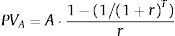
and the present value of a level annuity of amount A and length T is given by:Substituting these two equations into Eq. (6) and simplifying yields:Differentiating Eq. (A3) with respect to A yields:Duration is decreasing in the magnitude of the annuity with the rate of decrease being larger for longer forecast horizons, lower discount rates and lower stock valuations.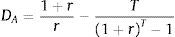

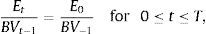
With respect to Eq. (8), if we assume that growth in equity is zero for all finite forecast periods, i.e.,
and perfect persistence of current ROE over the forecast period, i.e.,then Eq. (8) simplifies to:If the amount of the annuity for the finite forecast horizon is now equal to earnings at the beginning of the forecast horizon, Eq. (A3) becomes:Accordingly, we note that there is a negative relation between IED and the EPR. Therefore, EPR is a good proxy for equity duration in firms where growth in equity is low and ROE is highly persistent.

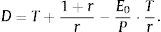
To see the relation between IED and BtM, the authors assume that growth in equity is again zero over the forecast period but that ROE immediately mean reverts to the cost of capital in the first year of the forecast period, i.e.,
Eq. (8) now simplifies to:The amount of the annuity for the finite forecast horizon is equal to book value at the beginning of the forecast horizon multiplied by the cost of capital. Thus, the implied equity duration becomes:In this special case, there is a simple negative relation between IED and BtM. The BtM ratio is a good proxy for duration for those firms where growth in equity is low and ROE rapidly reverts to its mean.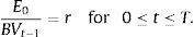

In the fixed income field, the duration concept has been widely used and developed up to the concept of duration vector to unobservable factors, extracted by principal component analysis (Benito, 2006) and independent component analysis (González and Nave, 2010) from the term structure of interest rates.
The financial sector idiosyncrasy regarding interest rates makes the separation between financial and non-financial firms necessary, giving rise to a parallel line of research on the sensitivity of financial firms to interest rate movements (Ballester et al., 2011).
An explanation for negative values for the IED is that the stock is underpriced or, alternatively, that the model incorrectly assumes that past profitability will continue into the future.
We use the parametric t-test after performing the Levene test for equality of variances. The non-parametric test we use is the U of Mann–Whitney test when normality is not rejected and the W Wilcoxon test, otherwise.
As the referee suggests, it would be interesting to add a regression of the same variables while controlling for the industrial sector as a robustness exercise. However, the few number of firms in some of the sectors (for example, in the Technology and Communications sector, only six companies are listed) does not allow us to do so.

