


In this article we present a theoretical review of the existing literature on Value at Risk (VaR) specifically focussing on the development of new approaches for its estimation. We effect a deep analysis of the State of the Art, from standard approaches for measuring VaR to the more evolved, while highlighting their relative strengths and weaknesses. We will also review the backtesting procedures used to evaluate VaR approach performance. From a practical perspective, empirical literature shows that approaches based on the Extreme Value Theory and the Filtered Historical Simulation are the best methods for forecasting VaR. The Parametric method under skewed and fat-tail distributions also provides promising results especially when the assumption that standardised returns are independent and identically distributed is set aside and when time variations are considered in conditional high-order moments. Lastly, it appears that some asymmetric extensions of the CaViaR method provide results that are also promising.
Basel I, also called the Basel Accord, is the agreement reached in 1988 in Basel (Switzerland) by the Basel Committee on Bank Supervision (BCBS), involving the chairmen of the central banks of Germany, Belgium, Canada, France, Italy, Japan, Luxembourg, Netherlands, Spain, Sweden, Switzerland, the United Kingdom and the United States of America. This accord provides recommendations on banking regulations with regard to credit, market and operational risks. Its purpose is to ensure that financial institutions hold enough capital on account to meet obligations and absorb unexpected losses.
For a financial institution measuring the risk it faces is an essential task. In the specific case of market risk, a possible method of measurement is the evaluation of losses likely to be incurred when the price of the portfolio assets falls. This is what Value at Risk (VaR) does. The portfolio VaR represents the maximum amount an investor may lose over a given time period with a given probability. Since the BCBS at the Bank for International Settlements requires a financial institution to meet capital requirements on the basis of VaR estimates, allowing them to use internal models for VaR calculations, this measurement has become a basic market risk management tool for financial institutions.2 Consequently, it is not surprising that the last decade has witnessed the growth of academic literature comparing alternative modelling approaches and proposing new models for VaR estimations in an attempt to improve upon those already in existence.
Although the VaR concept is very simple, its calculation is not easy. The methodologies initially developed to calculate a portfolio VaR are (i) the variance–covariance approach, also called the Parametric method, (ii) the Historical Simulation (Non-parametric method) and (iii) the Monte Carlo simulation, which is a Semi-parametric method. As is well known, all these methodologies, usually called standard models, have numerous shortcomings, which have led to the development of new proposals (see Jorion, 2001).
Among Parametric approaches, the first model for VaR estimation is Riskmetrics, from Morgan (1996). The major drawback of this model is the normal distribution assumption for financial returns. Empirical evidence shows that financial returns do not follow a normal distribution. The second relates to the model used to estimate financial return conditional volatility. The third involves the assumption that return is independent and identically distributed (iid). There is substantial empirical evidence to demonstrate that standardised financial returns distribution is not iid.
Given these drawbacks research on the Parametric method has moved in several directions. The first involves finding a more sophisticated volatility model capturing the characteristics observed in financial returns volatility. The second line of research involves searching for other density functions that capture skewness and kurtosis of financial returns. Finally, the third line of research considers that higher-order conditional moments are time-varying.
In the context of the Non-parametric method, several Non-parametric density estimation methods have been implemented, with improvement on the results obtained by Historical Simulation. In the framework of the Semi-parametric method, new approaches have been proposed: (i) the Filtered Historical Simulation, proposed by Barone-Adesi et al. (1999); (ii) the CaViaR method, proposed by Engle and Manganelli (2004) and (iii) the conditional and unconditional approaches based on the Extreme Value Theory. In this article, we will review the full range of methodologies developed to estimate VaR, from standard models to those recently proposed. We will expose the relative strengths and weaknesses of these methodologies, from both theoretical and practical perspectives. The article's objective is to provide the financial risk researcher with all the models and proposed developments for VaR estimation, bringing him to the limits of knowledge in this field.
The paper is structured as follows. In the next section, we review a full range of methodologies developed to estimate VaR. In Section 2.1, a non-parametric approach is presented. Parametric approaches are offered in Section 2.2, and semi-parametric approaches in Section 2.3. In Section 3, the procedures for measuring VaR adequacy are described and in Section 4, the empirical results obtained by papers dedicated to comparing VaR methodologies are shown. In Section 5, some important topics of VaR are discussed. The last section presents the main conclusions.
2Value at Risk methodsAccording to Jorion (2001), “VaR measure is defined as the worst expected loss over a given horizon under normal market conditions at a given level of confidence. For instance, a bank might say that the daily VaR of its trading portfolio is $1 million at the 99 percent confidence level. In other words, under normal market conditions, only one percent of the time, the daily loss will exceed $1 million.” In fact the VaR just indicates the most we can expect to lose if no negative event occurs.
The VaR is thus a conditional quantile of the asset return loss distribution. Among the main advantages of VaR are simplicity, wide applicability and universality (see Jorion, 1990, 1997).3 Let r1, r2, r3,…, rn be identically distributed independent random variables representing the financial returns. Use F(r) to denote the cumulative distribution function, F(r)=Pr(r<r|Ωt−1) conditionally on the information set Ωt−1 that is available at time t−1. Assume that {rt} follows the stochastic process:
where σt2=E(zt2|Ωt−1) and zt has the conditional distribution function G(z),G(z)=Pr(zt
This quantile can be estimated in two different ways: (1) inverting the distribution function of financial returns, F(r), and (2) inverting the distribution function of innovations, with regard to G(z) the latter, it is also necessary to estimate σt2.

Hence, a VaR model involves the specifications of F(r) or G(z). The estimation of these functions can be carried out using the following methods: (1) non-parametric methods; (2) parametric methods and (3) semi-parametric methods. Below we will describe the methodologies, which have been developed in each of these three cases to estimate VaR.4
2.1Non-parametric methodsThe Non-parametric approaches seek to measure a portfolio VaR without making strong assumptions about returns distribution. The essence of these approaches is to let data speak for themselves as much as possible and to use recent returns empirical distribution – not some assumed theoretical distribution – to estimate VaR.
All Non-parametric approaches are based on the underlying assumption that the near future will be sufficiently similar to the recent past for us to be able to use the data from the recent past to forecast the risk in the near future.
The Non-parametric approaches include (a) Historical Simulation and (b) Non-parametric density estimation methods.
2.1.1Historical simulationHistorical Simulation is the most widely implemented Non-parametric approach. This method uses the empirical distribution of financial returns as an approximation for F(r), thus VaR(α) is the α quantile of empirical distribution. To calculate the empirical distribution of financial returns, different sizes of samples can be considered.
The advantages and disadvantages of the Historical Simulation have been well documented by Down (2002). The two main advantages are as follows: (1) the method is very easy to implement, and (2) as this approach does not depend on parametric assumptions on the distribution of the return portfolio, it can accommodate wide tails, skewness and any other non-normal features in financial observations. The biggest potential weakness of this approach is that its results are completely dependent on the data set. If our data period is unusually quiet, Historical Simulation will often underestimate risk and if our data period is unusually volatile, Historical Simulation will often overestimate it. In addition, Historical Simulation approaches are sometimes slow to reflect major events, such as the increases in risk associated with sudden market turbulence.
The first papers involving the comparison of VaR methodologies, such as those by Beder (1995, 1996), Hendricks (1996), and Pritsker (1997), reported that the Historical Simulation performed at least as well as the methodologies developed in the early years, the Parametric approach and the Monte Carlo simulation. The main conclusion of these papers is that among the methodologies developed initially, no approach appeared to perform better than the others.
However, more recent papers such as those by Abad and Benito (2013), Ashley and Randal, 2009, Trenca (2009), Angelidis et al. (2007), Alonso and Arcos (2005), Gento (2001), Danielsson and de Vries (2000) have reported that the Historical Simulation approach produces inaccurate VaR estimates. In comparison with other recently developed methodologies such as the Historical Simulation Filtered, Conditional Extreme Value Theory and Parametric approaches (as we become further separated from normality and consider volatility models more sophisticated than Riskmetrics), Historical Simulation provides a very poor VaR estimate.
2.1.2Non-parametric density estimation methodsUnfortunately, the Historical Simulation approach does not best utilise the information available. It also has the practical drawback that it only gives VaR estimates at discrete confidence intervals determined by the size of our data set.5 The solution to this problem is to use the theory of Non-parametric density estimation. The idea behind Non-parametric density is to treat our data set as if it were drawn from some unspecific or unknown empirical distribution function. One simple way to approach this problem is to draw straight lines connecting the mid-points at the top of each histogram bar. With these lines drawn the histogram bars can be ignored and the area under the lines treated as though it was a probability density function (pdf) for VaR estimation at any confidence level. However, we could draw overlapping smooth curves and so on. This approach conforms exactly to the theory of non-parametric density estimation, which leads to important decisions about the width of bins and where bins should be centred. These decisions can therefore make a difference to our results (for a discussion, see Butler and Schachter (1998) or Rudemo (1982)).
A kernel density estimator (Silverman, 1986; Sheather and Marron, 1990) is a method for generalising a histogram constructed with the sample data. A histogram results in a density that is piecewise constant where a kernel estimator results in smooth density. Smoothing the data can be performed with any continuous shape spread around each data point. As the sample size grows, the net sum of all the smoothed points approaches the true pdf whatever that may be irrespective of the method used to smooth the data.
The smoothing is accomplished by spreading each data point with a kernel, usually a pdf centred on the data point, and a parameter called the bandwidth. A common choice of bandwidth is that proposed by Silverman (1986). There are many kernels or curves to spread the influence of each point, such as the Gaussian kernel density estimator, the Epanechnikov kernel, the biweight kernel, an isosceles triangular kernel and an asymmetric triangular kernel. From the kernel, we can calculate the percentile or estimate of the VaR.
2.2Parametric methodParametric approaches measure risk by fitting probability curves to the data and then inferring the VaR from the fitted curve. Among Parametric approaches, the first model to estimate VaR was Riskmetrics from Morgan (1996). This model assumes that the return portfolio and/or the innovations of return follow a normal distribution. Under this assumption, the VaR of a portfolio at an 1−α% confidence level is calculated as VaR(α)=μ+σtG−1(α), where G−1(α) is the α quantile of the standard normal distribution and σt is the conditional standard deviation of the return portfolio. To estimate σt, Morgan uses an Exponential Weight Moving Average Model (EWMA). The expression of this model is as follows:
where λ=0.94 and the window size (N) is 74 days for daily data.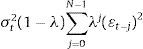
The major drawbacks of Riskmetrics are related to the normal distribution assumption for financial returns and/or innovations. Empirical evidence shows that financial returns do not follow normal distribution. The skewness coefficient is in most cases negative and statistically significant, implying that the financial return distribution is skewed to the left. This result is not in accord with the properties of a normal distribution, which is symmetric. Also, empirical distribution of financial return has been documented to exhibit significantly excessive kurtosis (fat tails and peakness) (see Bollerslev, 1987). Consequently, the size of the actual losses is much higher than that predicted by a normal distribution.
The second drawback of Riskmetrics involves the model used to estimate the conditional volatility of the financial return. The EWMA model captures some non-linear characteristics of volatility, such as varying volatility and cluster volatility, but does not take into account asymmetry and the leverage effect (see Black, 1976; Pagan and Schwert, 1990). In addition, this model is technically inferior to the GARCH family models in modelling the persistence of volatility.
The third drawback of the traditional Parametric approach involves the iid return assumption. There is substantial empirical evidence that the standardised distribution of financial returns is not iid (see Hansen, 1994; Harvey and Siddique, 1999; Jondeau and Rockinger, 2003; Bali and Weinbaum, 2007; Brooks et al., 2005).
Given these drawbacks research on the Parametric method has been made in several directions. The first attempts searched for a more sophisticated volatility model capturing the characteristics observed in financial returns volatility. Here, three families of volatility models have been considered: (i) the GARCH, (ii) stochastic volatility and (iii) realised volatility. The second line of research investigated other density functions that capture the skew and kurtosis of financial returns. Finally, the third line of research considered that the higher-order conditional moments are time-varying.
Using the Parametric method but with a different approach, McAleer et al. (2010a) proposed a risk management strategy consisting of choosing from among different combinations of alternative risk models to measure VaR. As the authors remark, given that a combination of forecast models is also a forecast model, this model is a novel method for estimating the VaR. With such an approach McAleer et al. (2010b) suggest using a combination of VaR forecasts to obtain a crisis robust risk management strategy. McAleer et al. (2011) present cross-country evidence to support the claim that the median point forecast of VaR is generally robust to a Global Financial Crisis.
2.2.1Volatility modelsThe volatility models proposed in literature to capture the characteristics of financial returns can be divided into three groups: the GARCH family, the stochastic volatility models and realised volatility-based models. As to the GARCH family, Engle (1982) proposed the Autoregressive Conditional Heterocedasticity (ARCH), which featured a variance that does not remain fixed but rather varies throughout a period. Bollerslev (1986) further extended the model by inserting the ARCH generalised model (GARCH). This model specifies and estimates two equations: the first depicts the evolution of returns in accordance with past returns, whereas the second patterns the evolving volatility of returns. The most generalised formulation for the GARCH models is the GARCH (p,q) model represented by the following expression:
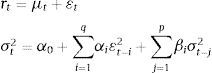
In the GARCH (1,1) model, the empirical applications conducted on financial series detect that α1+β1 is observed to be very close to the unit. The integrated GARCH model (IGARCH) of Engle and Bollerslev (1986)6 is then obtained forcing the condition that the addition is equal to the unit in expression (4). The conditional variance properties of the IGARCH model are not very attractive from the empirical point of view due to the very slow phasing out of the shock impact upon the conditional variance (volatility persistence). Nevertheless, the impacts that fade away show exponential behaviour, which is how the fractional integrated GARCH model (FIGARCH) proposed by Baillie et al. (1996) behaves, with the simplest specification, FIGARCH (1, d, 0), being:
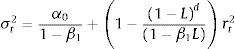
If the parameters comply with the setting conditions α0>0,0≤β1
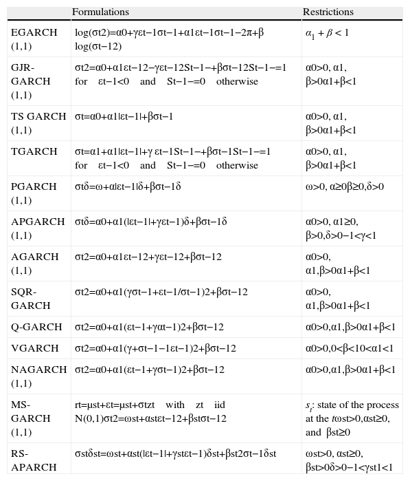
The models previously mentioned do not completely reflect the nature posed by the volatility of the financial times series because, although they accurately characterise the volatility clustering properties, they do not take into account the asymmetric performance of yields before positive or negative shocks (leverage effect). Because previous models depend on the square errors, the effect caused by positive innovations is the same as the effect produced by negative innovations of equal absolute value. Nonetheless, reality shows that in financial time series, the existence of the leverage effect is observed, which means that volatility increases at a higher rate when yields are negative compared with when they are positive. In order to capture the leverage effect several non-linear GARCH formulations have been proposed. In Table 1, we present some of the most popular. For a detailed review of the asymmetric GARCH models (see Bollerslev, 2009).
Asymmetric GARCH.
| Formulations | Restrictions | |
| EGARCH (1,1) | log(σt2)=α0+γεt−1σt−1+α1εt−1σt−1−2π+β log(σt−12) | α1+β<1 |
| GJR-GARCH (1,1) | σt2=α0+α1εt−12−γεt−12St−1−+βσt−12St−1−=1 for εt−1<0 and St−1−=0 otherwise | α0>0, α1, β>0α1+β<1 |
| TS GARCH (1,1) | σt=α0+α1|εt−1|+βσt−1 | α0>0, α1, β>0α1+β<1 |
| TGARCH | σt=α1+α1|εt−1|+γ εt−1St−1−+βσt−1St−1−=1 for εt−1<0 and St−1−=0 otherwise | α0>0, α1, β>0α1+β<1 |
| PGARCH (1,1) | σtδ=ω+α|εt−1|δ+βσt−1δ | ω>0, α≥0β≥0,δ>0 |
| APGARCH (1,1) | σtδ=α0+α1(|εt−1|+γεt−1)δ+βσt−1δ | α0>0, α1≥0, β>0,δ>0−1<γ<1 |
| AGARCH (1,1) | σt2=α0+α1εt−12+γεt−12+βσt−12 | α0>0, α1,β>0α1+β<1 |
| SQR-GARCH | σt2=α0+α1(γσt−1+εt−1/σt−1)2+βσt−12 | α0>0, α1,β>0α1+β<1 |
| Q-GARCH | σt2=α0+α1(εt−1+γαt−1)2+βσt−12 | α0>0,α1,β>0α1+β<1 |
| VGARCH | σt2=α0+α1(γ+σt−1−1εt−1)2+βσt−12 | α0>0,0<β<10<α1<1 |
| NAGARCH (1,1) | σt2=α0+α1(εt−1+γσt−1)2+βσt−12 | α0>0,α1,β>0α1+β<1 |
| MS-GARCH (1,1) | rt=μst+εt=μst+σtzt with zt iid N(0,1)σt2=ωst+αstεt−12+βstσt−12 | st: state of the process at the tωst>0,αst≥0, and βst≥0 |
| RS-APARCH | σstδst=ωst+αst(|εt−1|+γstεt−1)δst+βst2σt−1δst | ωst>0, αst≥0, βst>0δ>0−1<γst1<1 |
In all models presented in this table, γ is the leverage parameter. A negative value of γ means that past negative shocks have a deeper impact on current conditional volatility than past positive shocks. Thus, we expect the parameter to be negative (γ<0). The persistence of volatility is captured by the β parameter. As for the EGARCH model, the volatility of return also depends on the size of innovations. If α1 is positive, the innovations superior to the mean have a deeper impact on current volatility than those inferior.
Finally, it must be pointed out that there are some models that capture the leverage effect and the non-persistence memory effect. For example, Bollerslev and Mikkelsen (1996) insert the FIEGARCH model, which aims to account for both the leveraging effect (EGARCH) and the long memory (FIGARCH) effect. The simplest expression of this family of models is the FIEGARCH (1, d, 0):

Some applications of the family of GARCH models in VaR literature can be found in the following studies: Abad and Benito (2013), Sener et al. (2012), Chen et al. (2009, 2011), Sajjad et al. (2008), Bali and Theodossiou (2007), Angelidis et al. (2007), Haas et al. (2004), Li and Lin (2004), Carvalho et al. (2006), González-Rivera et al. (2004), Giot and Laurent (2004), Mittnik and Paolella (2000), among others. Although there is no evidence of an overpowering model, the results obtained in these papers seem to indicate that asymmetric GARCH models produce better outcomes.
An alternative path to the GARCH models to represent the temporal changes over volatility is through the stochastic volatility (SV) models proposed by Taylor (1982, 1986). Here volatility in t does not depend on the past observations of the series but rather on a non-observable variable, which is usually an autoregressive stochastic process. To ensure the positiveness of the variance, the volatility equation is defined following the logarithm of the variance as in the EGARCH model.
The stochastic volatility model proposed by Taylor (1982) can be written as:
where μt represents the conditional mean of the financial return, ht represents the conditional variance, and zt and ηt are stochastic white-noise processes.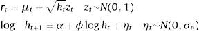
The basic properties of the model can be found in Taylor (1986, 1994). As in the GARCH family, alternative and more complex models have been developed for the stochastic volatility models to allow for the pattern of both the large memory (see the model of Harvey (1998) and Breidt et al. (1998)) and the leverage effect (see the models of Harvey and Shephard (1996) and So et al. (2002)). Some applications of the SV model to measure VaR can be found in Fleming and Kirby (2003), Lehar et al. (2002), Chen et al. (2011) and González-Rivera et al. (2004).
The third group of volatility models is realised volatility (RV). The origin of the realised volatility concept is certainly not recent. Merton (1980) had already mentioned this concept, showing the likelihood of the latent volatility approximation by the addition of N intra-daily square yields over a t period, thus implying that the addition of square yields could be used for the variance estimation. Taylor and Xu (1997) showed that the daily realised volatility can be easily crafted by adding the intra-daily square yields. Assuming that a day is divided into equidistant N periods and if ri,t represents the intra-daily yield of the i-interval of day t, the daily volatility for day t can be expressed as:

In the event of yields with “zero” mean and no correlation whatsoever, then E∑i=1Nri,t2 is a consistent estimator of the daily variance σt2Andersen et al. (2001a,b) upheld that this measure significantly improves the forecast compared with the standard procedures, which just rely on daily data.
Although financial yields clearly exhibit leptokurtosis, the standardised yields by realised volatility are roughly normal. Furthermore, although the realised volatility distribution poses a clear asymmetry to the right, the distributions of the realised volatility logarithms are approximately Gaussian (Pong et al. (2004)). In addition, the long-term dynamics of the realised volatility logarithm can be inferred by a fractionally integrated long memory process. The theory suggests that realised volatility is a non-skewed estimator of the volatility yields and is highly efficient. The use of the realised volatility obtained from the high-frequency intra-daily yields allows for the use of traditional procedures of temporal times series to create patterns and forecasts.
One of the most representative realised volatility models is that proposed by Pong et al. (2004):

As in the case of GARCH family models and stochastic volatility models, some extension of the standard RV model have been developed in order to capture the leverage effect and long-range dependence of volatility. The former issue has been investigated by Bollerslev et al. (2011), Chen and Ghysels (2010), Patton and Sheppard (2009), among others. With respect to the latter point, the autoregressive fractionally integrated model has been used by Andersen et al. (2001a, 2001b, 2003), Koopman et al. (2005), Pong et al. (2004), among others.
- a)
Empirical results of volatility models in VaR
This section lists the results obtained from research on the comparison of volatility models in terms of VaR. The EWMA model provides inaccurate VaR estimates. In a comparison with other volatility models, the EWMA model scored the worst performance in forecasting VaR (see Chen et al., 2011; Abad and Benito, 2013; Ñíguez, 2008; Alonso and Arcos, 2006; González-Rivera et al., 2004; Huang and Lin, 2004 and among others). The performance of the GARCH models strongly depends on the assumption concerning returns distribution. Overall, under a normal distribution, the VaR estimates are not very accurate. However, when asymmetric and fat-tail distributions are considered, the results improve considerably.
There is scarce empirical evidence of the relative performance of the SV models against the GARCH models in terms of VaR (see Fleming and Kirby, 2003; Lehar et al., 2002; González-Rivera et al., 2004; Chen et al., 2011). Fleming and Kirby (2003) compared a GARCH model with a SV model. They found that both models had comparable performances in terms of VaR. Lehar et al. (2002) compared option pricing models in terms of VaR using two family models: GARCH and SV. They found that as to their ability to forecast the VaR, there are no differences between the two. Chen et al. (2011) compared the performance of two SV models with a range wide of GARCH family volatility models. The comparison was conducted on two different samples. They found that the SV and EWMA models had the worst performances in estimating VaR. However, in a similar comparison, González-Rivera et al. (2004) found that the SV model had the best performance in estimating VaR. In general, with some exceptions, evidence suggests that SV models do not improve the results obtained GARCH model family.
The models based on RV work quite well to estimate VaR (see Asai et al., 2011; Brownlees and Gallo, 2010; Clements et al., 2008; Giot and Laurent, 2004; Andersen et al., 2003). Some papers show that an even simpler model (such as an autoregressive), combined with the assumption of normal distribution for returns, yields reasonable VaR estimates.
As for volatility forecasts, there are many papers in literature showing that the models based on RV are superior to the GARCH models. However, not many papers report comparisons on their ability to forecast VaR. Brownlees and Gallo (2011) compared several RV models with a GARCH and EWMA model and found that the models based on RV outperformed both EWMA and GARCH models. Along this same line, Giot and Laurent (2004) compared several volatility models: EWMA, an asymmetric GARCH and RV. The models are estimated with the assumption that returns follow either normal or skewed t-Student distributions. They found that under a normal distribution, the RV model performed best. However, under a skewed t-distribution, the asymmetric GARCH and RV models provided very similar results. These authors emphasised that the superiority of the models based on RV over the GARCH family is not as obvious when the estimation of the latter assumes the existence of asymmetric and leptokurtic distributions.
There is a lack of empirical evidence on the performance of fractional integrated volatility models to measure VaR. Examples of papers that report comparisons of these models are those by So and Yu (2006) and Beltratti and Morana (1999). The first paper compared, in terms of VaR, a FIGARCH model with a GARCH and an IGARCH model. It showed that the GARCH model provided more accurate VaR estimates. In a similar comparison that included the EWMA model, So and Yu (2006) found that FIGARCH did not outperform GARCH. The authors concluded that, although their correlation plots displayed some indication of long memory volatility, this feature is not very crucial in determining the proper value of VaR. However, in the context of the RV models, there is evidence that models that capture long memory in volatility provide accurate VaR estimates (see Andersen et al., 2003; Asai et al., 2011). The model proposed by Asai et al. (2011) captured long memory volatility and asymmetric features. Along this line, Ñíguez (2008) compared the ability to forecast VaR of different GARCH family models (GARCH, AGARCH, APARCH, FIGARCH and FIAPARCH, and EWMA) and found that the combination of asymmetric models with fractional integrated models provided the best results.
Although this evidence is somewhat ambiguous, the asymmetric GARCH models seem to provide better VaR estimations than the symmetric GARCH models. Evidence in favour of this hypothesis can be found in studies by Sener et al. (2012), Bali and Theodossiou (2007), Abad and Benito (2013), Chen et al. (2011), Mittnik and Paolella (2000), Huang and Lin (2004), Angelidis et al. (2007), and Giot and Laurent (2004). In the context of the models based on RV, the asymmetric models also provide better results (see Asai et al., 2011). Some evidence against this hypothesis can be found in Angelidis et al. (2007).
Finally, some authors state that the assumption of distribution, not the volatility models, is actually the important factor for estimating VaR. Evidence supporting this issue is found in the study by Chen et al. (2011).
2.2.2Density functionsAs previously mentioned, the empirical distribution of the financial return has been documented to be asymmetric and exhibits a significant excess of kurtosis (fat tail and peakness). Therefore, assuming a normal distribution for risk management and particularly for estimating the VaR of a portfolio does not produce good results and losses will be much higher.
As t-Student distribution has fatter tails than normal distribution, this distribution has been commonly used in finance and risk management, particularly to model conditional asset return (Bollerslev, 1987). In the context of VaR methodology, some applications of this distribution can be found in studies by Cheng and Hung (2011), Abad and Benito (2013), Polanski and Stoja (2010), Angelidis et al. (2007), Alonso and Arcos (2006), Guermat and Harris (2002), Billio and Pelizzon (2000), and Angelidis and Benos (2004). The empirical evidence of this distribution performance in estimating VaR is ambiguous. Some papers show that the t-Student distribution performs better than the normal distribution (see Abad and Benito, 2013; Polanski and Stoja, 2010; Alonso and Arcos, 2006; So and Yu, 20067). However other papers, such as those by Angelidis et al. (2007), Guermat and Harris (2002), Billio and Pelizzon (2000), and Angelidis and Benos (2004), report that the t-Student distribution overestimates the proportion of exceptions.
The t-Student distribution can often account well for the excess kurtosis found in common asset returns, but this distribution does not capture the skewness of the return. Taking this into account, one direction for research in risk management involves searching for other distribution functions that capture these characteristics. In the context of VaR methodology, several density functions have been considered: the Skewness t-Student Distribution (SSD) of Hansen (1994); Exponential Generalised Beta of the Second Kind (EGB2) of McDonald and Xu (1995); Error Generalised Distribution (GED) of Nelson (1991); Skewness Error Generalised Distribution (SGED) of Theodossiou (2001); t-Generalised Distribution of McDonald and Newey (1988); Skewness t-Generalised distribution (SGT) of Theodossiou (1998) and Inverse Hyperbolic Sign (IHS) of Johnson (1949). In Table 2, we present the density functions of these distributions.
Density functions.
| Formulations | Restrictions | ||
| Skewness t-Student distribution (SSD) of Hansen (1994) | f(zt|v,η)=bc1+1η−2bzt+a1−η2−(η+1)/2if zt<−abbc1+1η−2bzt+a1+η2−(η+1)/2if zt≥−ab | a=4λcη−2η−2b2=1+3λ2−a2c=Γη+12π(η−2) Γη2zt=(rt−μt)/σt | |λ|<1η>2 |
| Beta Exponential Generalised of the Second Kind (EGB2) McDonald and Xu (1995) | EGB2(zt;p;q)=Cep(zt+δ)/θ)1+ep(zt+δ)/θ)p+q | C=1/(B(p,q)θ) δ=(Ψ(p)−Ψ(q))θθ=1/Ψ′(p)+Ψ′(q) zt=(rt−μt)/σt | p=q EGB2 symmetricp>q positively skewedp>q negatively skewed |
| Error Generalised (GED) of Nelson (1991) | f(zt)=ηλ2(1+1/η)Γ(1/η)exp−12ztλη | λ≡2(−2/v)Γ1η/Γ3ηzt=(rt−μt)/σt0.5 | −∞ |
| Skewness Generalised Error (SGED) of Theodossiou (2001) | f(zt|λ,k)=Cσexp−|zt+δ|k(1+sign(zt+δ)λ)kθk | zt=(rt−μt)/σtC=k/(2θΓ(1/k)) δ=2λAS(λ)−1θ=Γ(1/k)0.5Γ(3/k)−0.5S(λ)−1δ=2λAS(λ)−1 S(λ)=1+3λ2−4A2λ2 | |λ|<1 skewed parameterk=kurtosis parameter |
| t-Generalised Distribution (GT) of McDonald and Newey (1988) | f(zt|λ,h,k)=kΓ(h)2λΓ(1/k)Γ(h−1/k)1+|zt|λk−h | λ>0, k<0,h>0−∞ | |
| Skewness t-Generalised Distribution (SGT) of Theodossiou (1998) | f(zt|λ,η,k)=C1+|zt+δ|k((η+1)/k)(1+sign(zt+δ)λ)kθk−η+1/k | C=0,5kη+1k−1/kBηk,1k−1θ−1 θ=1g−ρ2ρ=2λBηk,1k−1η+1k1/kBη−1k,2kg=(1+3λ2)Bηk,1k−1η+1k1/kBη−1k,3k δ=ρθ | |λ|<1 skewed parameterη>2 tail-thickness parameterk>0 peakedness parameterδ Pearson's skewnesszt=(rt−μt)/σt |
| Inverse Hyperbolic sine (IHS) of Johnson (1949) | IHS(zt|λ,k)=−k2π(θ2+(zt+δ)2)×exp−k22ln(zt+δ)+θ2+(zt+δ)2−(λ+ln(θ)2 | θ=1/σw δ=μw/σwσw=0.5(e2λ+k−2+e−2λ+k−2+2)0.5(ek−2−1) | μw meanσw standard deviationw=sinh(λ+x/k)x standard normal variable |
In this line, some papers such as Duffie and Pan (1997) and Hull and White (1998) show that a mixture of normal distributions produces distributions with fatter tails than a normal distribution with the same variance.
Some applications to estimate the VaR of skewed distributions and a mixture of normal distributions can be found in Cheng and Hung (2011), Polanski and Stoja (2010), Bali and Theodossiou (2008), Bali et al. (2008), Haas et al. (2004), Zhang and Cheng (2005), Haas (2009), Ausín and Galeano (2007), Xu and Wirjanto (2010) and Kuester et al. (2006).
These papers raise some important issues. First, regarding the normal and t-Student distributions, the skewed and fat-tail distributions seem to improve the fit of financial data (see Bali and Theodossiou, 2008; Bali et al., 2008; Bali and Theodossiou, 2007). Consistently, some studies found that the VaR estimate obtained under skewed and fat-tailed distributions provides a more accurate VaR than those obtained from a normal or t-Student distribution. For example, Cheng and Hung (2011) compared the ability to forecast the VaR of a normal, t-Student, SSD and GED. In this comparison the SSD and GED distributions provide the best results. Polanski and Stoja (2010) compared the normal, t-Student, SGT and EGB2 distributions and found that just the latter two distributions provide accurate VaR estimates. Bali and Theodossiou (2007) compared a normal distribution with the SGT distribution. Again, they found that the SGT provided a more accurate VaR estimate. The main disadvantage of using some skewness distribution, such as SGT, is that the maximisation of the likelihood function is very complicated so that it may take a lot of computational time (see Nieto and Ruiz, 2008).
Additionally, a mixture of normal distributions, t-Student distributions or GED distributions provided a better VaR estimate than the normal or t-Student distributions (see Hansen, 1994; Zhang and Cheng, 2005; Haas, 2009; Ausín and Galeano, 2007; Xu and Wirjanto, 2010; Kuester et al., 2006). These studies showed that in the context of the Parametric method, the VaR estimations obtained with models involving a mixture with normal distributions (and t-Student distributions) are generally quite precise.
Lastly, to handle the non-normality of the financial return Hull and White (1998) develop a new model where the user is free to choose any probability distribution for the daily return and the parameters of the distribution are subject to an updating scheme such as GARCH. They propose transforming the daily return into a new variable that is normally distributed. The model is appealing in that the calculation of VaR is relatively straightforward and can make use of Riskmetrics or a similar database.
2.2.3Higher-order conditional time-varying momentsThe traditional parametric approach for conditional VaR assumes that the distribution of returns standardised by conditional means and conditional standard deviations is iid. However, there is substantial empirical evidence that the distribution of financial returns standardised by conditional means and volatility is not iid. Earlier studies also suggested that the process of negative extreme returns at different quantiles may differ from one another (Engle and Manganelli, 2004; Bali and Theodossiou, 2007). Thus, given the above, some studies developed a new approach to calculate conditional VaR. This new approach considered that the higher-order conditional moments are time-varying (see Bali et al., 2008; Polanski and Stoja, 2010; Ergun and Jun, 2010).
Bali et al. (2008) introduced a new method based on the SGT with time-varying parameters. They allowed higher-order conditional moment parameters of the SGT density to depend on the past information set and hence relax the conventional assumption in the conditional VaR calculation that the distribution of standardised returns is iid. Following Hansen (1994) and Jondeau and Rockinger (2003), they modelled the conditional high-order moment parameters of the SGT density as an autoregressive process. The maximum likelihood estimates show that the time-varying conditional volatility, skewness, tail-thickness, and peakedness parameters of the SGT density are statistically significant. In addition, they found that the conditional SGT-GARCH models with time-varying skewness and kurtosis provided a better fit or returns than the SGT-GARCH models with constant skewness and kurtosis. In their paper, they applied this new approach to calculate the VaR. The in-sample and out-of-sample performance results indicated that the conditional SGT-GARCH approach with autoregressive conditional skewness and kurtosis provided very accurate and robust estimates of the actual VaR thresholds.
In a similar study, Ergun and Jun (2010) considered the SSD distribution, which they called the ARCD model, with a time-varying skewness parameter. They found that the GARCH-based models that take conditional skewness and kurtosis into account provided an accurate VaR estimate. Along this same line, Polanski and Stoja (2010) proposed a simple approach to forecast a portfolio VaR. They employed the Gram-Charlier expansion (GCE) augmenting the standard normal distribution with the first four moments, which are allowed to vary over time. The key idea was to employ the GCE of the standard normal density to approximate the probability distribution of daily returns in terms of cumulants.8 This approach provides a flexible tool for modelling the empirical distribution of financial data, which, in addition to volatility, exhibits time-varying skewness and leptokurtosis. This method provides accurate and robust estimates of the realised VaR. Despite its simplicity, their dataset outperformed other estimates that were generated by both constant and time-varying higher-moment models.
All previously mentioned papers compared their VaR estimates with the results obtained by assuming skewed and fat-tail distributions with constant asymmetric and kurtosis parameters. They found that the accuracy of the VaR estimates improved when time-varying asymmetric and kurtosis parameters are considered. These studies suggest that within the context of the Parametric method, techniques that model the dynamic performance of the high-order conditional moments (asymmetry and kurtosis) provide better results than those considering functions with constant high-order moments.
The Semi-parametric methods combine the Non-parametric approach with the Parametric approach. The most important Semi-parametric methods are Volatility-weight Historical Simulation, Filtered Historical Simulation (FHS), CaViaR method and the approach based on Extreme Value Theory.
2.3.1Volatility-weight historical simulationTraditional Historical Simulation does not take any recent changes in volatility into account. Thus, Hull and White (1998) proposed a new approach that combines the benefit of Historical Simulation with volatility models. The basic idea of this approach is to update the return information to take into account the recent changes in volatility.
Let rt,i be the historical return on asset i on day t in our historical sample, σt,i be the forecast of the volatility9 of the return on asset i for day t made at the end of t−1, and σT,i be our most recent forecast of the volatility of asset i. Then, we replace the return in our data set, rt,i, with volatility-adjusted returns, as given by:

According to this new approach, the VaR(α) is the α quantile of the empirical distribution of the volatility adjusted return (rt,i*).
This approach directly takes into account the volatility changes, whereas the Historical Simulation approach ignores them. Furthermore, this method produces a risk estimate that is appropriately sensitive to current volatility estimates. The empirical evidence presented by Hull and White (1998) indicates that this approach produces a VaR estimate superior to that of the Historical Simulation approach.
2.3.2Filtered Historical SimulationFiltered Historical Simulation was proposed by Barone-Adesi et al. (1999). This method combines the benefits of Historical Simulation with the power and flexibility of conditional volatility models.
Suppose we use Filtered Historical Simulation to estimate the VaR of a single-asset portfolio over a 1-day holding period. In implementing this method, the first step is to fit a conditional volatility model to our portfolio return data. Barone-Adesi et al. (1999) recommended an asymmetric GARCH model. The realised returns are then standardised by dividing each one by the corresponding volatility, zt=(εt/σt). These standardised returns should be independent and identically distributed and therefore be suitable for Historical Simulation. The third step consists of bootstrapping a large number L of drawings from the above sample set of standardised returns.
Assuming a 1-day VaR holding period, the third stage involves bootstrapping from our data set of standardised returns: we take a large number of drawings from this data set, which we now treat as a sample, replacing each one after it has been drawn and multiplying each such random drawing by the volatility forecast 1 day ahead:
where z* is the simulated standardised return. If we take M drawings, we therefore obtain a sample of M simulated returns. With this approach, the VaR(α) is the α% quantile of the simulated return sample.
Recent empirical evidence shows that this approach works quite well in estimating VaR (see Barone-Adesi and Giannopoulos, 2001; Barone-Adesi et al., 2002; Zenti and Pallotta, 2001; Pritsker, 2001; Giannopoulos and Tunaru, 2005). As for other methods, Zikovic and Aktan (2009), Angelidis et al. (2007), Kuester et al. (2006) and Marimoutou et al. (2009) provide evidence that this method is the best for estimating the VaR. However, other papers indicate that this approach is not better than any other (see Nozari et al., 2010; Alonso and Arcos, 2006).
2.3.3CAViaR modelEngle and Manganelli (2004) proposed a conditional autoregressive specification for VaR. This approach is based on a quantile estimation. Instead of modelling the entire distribution, they proposed directly modelling the quantile. The empirical fact that the volatilities of stock market returns cluster over time may be translated quantitatively in that their distribution is autocorrelated. Consequently, the VaR, which is tightly linked to the standard deviation of the distribution, must exhibit similar behaviour. A natural way to formalise this characteristic is to use some type of autoregressive specification. Thus, they proposed a conditional autoregressive quantile specification that they called the CAViaR model.
Let rt be a vector of time t observable financial return and βα a p-vector of unknown parameters. Finally, let VaRt(β)≡VaRt(rt−1,βα) be the α quantile of the distribution of the portfolio return formed at time t−1, where we suppress the α subscript from βα for notational convenience.
A generic CAViaR specification might be the following:
where p=q+r+1 is the dimension of β and l is a function of a finite number of lagged observable values. The autoregressive terms βiVaRt−i (β) i=1,…, q ensure that the quantile changes “smoothly” over time. The role of l(rt−1) is to link VaRt(β) to observable variables that belong to the information set. A natural choice for xt−1 is lagged returns. The advantage of this method is that it makes no specific distributional assumption on the return of the asset. They suggested that the first order is sufficient for practical use:

In the context of CAViaR model, different autoregressive specifications can be considered
- -
Symmetric absolute value (SAV):
- -
Indirect GARCH(1,1) (IG):


In these two models the effects of the extreme returns and the variance on the VaR measure are modelled symmetrically. To account for financial market asymmetry, via the leverage effect (Black, 1976), the SAV model was extended in Engle and Manganelli (2004) to asymmetric slope (AS):

In this representation, (r)+=max(rt,0) and (rt)−=−min(rt,0) are used as the functions.
The parameters of the CAViaR models are estimated by regression quantiles, as introduced by Koenker and Basset (1978). They showed how to extend the notion of a sample quantile to a linear regression model. In order to capture leverage effects and other nonlinear characteristics of the financial return, some extensions of the CAViaR model have been proposed. Yu et al. (2010) extend the CAViaR model to include the Threshold GARCH (TGARCH) model (an extension of the double threshold ARCH (DTARCH) of Li and Li (1996)) and a mixture (an extension of Wong and Li (2001)’s mixture ARCH). Recently, Chen et al. (2011) proposed a non-linear dynamic quantile family as a natural extension of the AS model.
Although empirical literature on CAViaR method is not extensive, the results seem to indicate that the CAViaR model proposed by Engle and Manganelli (2004) fails to provide accurate VaR estimate although it may provide accurate VaR estimates in a stable period (see Bao et al., 2006; Polanski and Stoja, 2009). However, some recent extensions of the CaViaR model such as those proposed by Gerlach et al. (2011) and Yu et al. (2010) work pretty well in estimating VaR. As in the case of the Parametric method, it appears that when use is made of an asymmetric version of the CaViaR model the VaR estimate notably improves. The paper of Sener et al. (2012) supports this hypothesis. In a comparison of several CaViaR models (asymmetric and symmetric) they find that the asymmetric CaViaR model outperforms the result from the standard CaViaR model. Gerlach et al. (2011) compared three CAViaR models (SAV, AS and Threshold CAViaR) with the Parametric method using different volatility GARCH family models (GARCH-Normal, GARCH-Student-t, GJR-GARCH, IGARCH, Riskmetric). At the 1% confidence level, the Threshold CAViaR model performs better than any other.
2.3.4Extreme Value TheoryThe Extreme Value Theory (EVT) approach focuses on the limiting distribution of extreme returns observed over a long time period, which is essentially independent of the distribution of the returns themselves. The two main models for EVT are (1) the block maxima models (BM) (McNeil, 1998) and (2) the peaks-over-threshold model (POT). The second is generally considered to be the most useful for practical applications due to the more efficient use of the data at extreme values. In the POT models, there are two types of analysis: the Semi-parametric models built around the Hill estimator and its relatives (Beirlant et al., 1996; Danielsson et al., 1998) and the fully Parametric models based on the Generalised Pareto distribution (Embrechts et al., 1999). In the coming sections each one of these approaches is described.
2.3.4.1Block Maxima Models (BMM)This approach involves splitting the temporal horizon into blocks or sections, taking into account the maximum values in each period. These selected observations form extreme events, also called a maximum block.
The fundamental BMM concept shows how to accurately choose the length period, n, and the data block within that length. For values greater than n, the BMM provides a sequence of maximum blocks Mn,1,…, Mn,m that can be adjusted by a generalised distribution of extreme values (GEV). The maximum loss within a group of n data is defined as Mn=max(X1, X2,…, Xn).
For a group of identically distributed observations, the distribution function of Mn is represented as:

The asymptotic approach for Fn(x) is based on the maximum standardised value
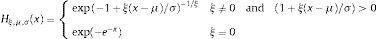
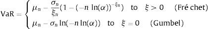
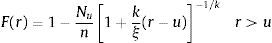
where μn and σn are the location and scale parameters, respectively. The theorem of Fisher and Tippet establishes that if Zn converges to a non-degenerated distribution, this distribution is the generalised distribution of the extreme values (GEV). The algebraic expression for such a generalised distribution is as follows:where σ>0, −∞<μ<∞, and −∞<ξ<∞. The parameter ξ is known as the shape parameter of the GEV distribution, and η=ξ−1 is the index of the tail distribution, H. The prior distribution is actually a generalisation of the three types of distributions, depending on the value taken by ξ: Gumbel type I family (ξ=0), Fréchet type II family (ξ>0) and Weibull type III family (ξ<0). The ξ, σ and μ parameters are estimated using maximum likelihood. The VaR expression for the Gumbel and Fréchet distribution is as follows:
In most situations, the blocks are selected in such a way that their length matches a year interval and n is the number of observations within that year period.
This method has been commonly used in hydrology and engineering applications but is not very suitable for financial time series due to the cluster phenomenon largely observed in financial returns.
2.3.4.2Peaks over threshold models (POT)The POT model is generally considered to be the most useful for practical applications due to the more efficient use of the data for the extreme values. In this model, we can distinguish between two types of analysis: (a) the fully Parametric models based on the Generalised Pareto distribution (GPD) and (b) the Semi-parametric models built around the Hill estimator.
- (a)
Generalised Pareto Distribution
Among the random variables representing financial returns (r1, r2, r3,…, rn), we choose a low threshold u and examine all values (y) exceeding u: (y1,y2,y3,…,yNu), where yi=ri−u and Nu are the number of sample data greater than u. The distribution of excess losses over the threshold u is defined as:
Assuming that for a certain u, the distribution of excess losses above the threshold is a Generalised Pareto Distribution, Gk,ξ(y)=1−[1+(k/ξ)y]−1/k, the distribution function of returns is given by:
To construct a tail estimator from this expression, the only additional element we need is an estimation of F(u). For this purpose, we take the obvious empirical estimator (u−Nu)/u. We then use the historical simulation method. Introducing the historical simulation estimate of F(u) and setting r=y+u in the equation, we arrive at the tail estimator
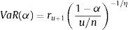
For a given probability α>F(u), the VaR estimate is calculated by inverting the tail estimation formula to obtain
None of the previous Extreme Value Theory-based methods for quantile estimation yield VaR estimates that reflect the current volatility background. These methods are called Unconditional Extreme Value Theory methods. Given the conditional heteroscedasticity characteristic of most financial data, McNeil and Frey (2000) proposed a new methodology to estimate the VaR that combines the Extreme Value Theory with volatility models, known as the Conditional Extreme Value Theory. These authors proposed GARCH models to estimate the current volatility and Extreme Value Theory to estimate the distributions tails of the GARCH model shocks.
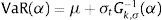
If the financial returns are a strictly stationary time series and ¿ follows a Generalised Pareto Distribution, denoted by Gk,σ (¿), the conditional α quantile of the returns can be estimated as
where σt2 represents the conditional variance of the financial returns and Gk,σ−1(α) is the α quantile of the GPD, which can be calculated as: - (b)
Hill estimator
The parameter that collects the features of the tail distribution is the tail index, η=ξ−1. Hill proposed a definition of the tail index as follows:
where ru represents the threshold return and u is the number of observations equal to or less than the threshold return. Thus, the Hill estimator is the mean of the most extreme u observations minus u+1 observations (ru+1). Additionally, the associated quantile estimator is (see Danielsson and de Vries, 2000):


The problem posed by this estimator is the lack of any analytical means to choose the threshold value of u in an optimum manner. Hence, as an alternative, the procedure involves using the feature known as Hill graphics. Different values of the Hill index are calculated for different u values; the Hill estimator values become represented in a chart or graphic based on u, and the u value is selected from the region where the Hill estimators are relatively stable (Hill chart leaning almost horizontally). The underlying intuitive idea posed in the Hill chart is that as u increases, the estimator variance decreases, and thus, the bias is increased. Therefore, the ability to foresee a balance between both trends is likely. When this level is reached, the estimator remains constant.
Existing literature on EVT models to calculate VaR is abundant. Regarding BMM, Silva and Melo (2003) considered different maximum block widths, with results suggesting that the extreme value method of estimating the VaR is a more conservative approach for determining the capital requirements than traditional methods. Byström (2004) applied both unconditional and conditional EVT models to the management of extreme market risks in the stock market and found that conditional EVT models provided particularly accurate VaR measures. In addition, a comparison with traditional Parametric (GARCH) approaches to calculate the VaR demonstrated EVT as being the superior approach for both standard and more extreme VaR quantiles. Bekiros and Georgoutsos (2005) conducted a comparative evaluation of the predictive performance of various VaR models, with a special emphasis on two methodologies related to the EVT, POT and BM. Their results reinforced previous results and demonstrated that some “traditional” methods might yield similar results at conventional confidence levels but that the EVT methodology produces the most accurate forecasts of extreme losses at very high confidence levels. Tolikas et al. (2007) compared EVT with traditional measures (Parametric method, HS and Monte Carlo) and agreed with Bekiros and Georgoutsos (2005) on the outperformance of the EVT methods compared with the rest, especially at very high confidence levels. The only model that had a performance comparable with that of the EVT is the HS model.
Some papers showed that unconditional EVT works better than the traditional HS or Parametric approaches when a normal distribution for returns is assumed and a EWMA model is used to estimate the conditional volatility of the return (see Danielsson and de Vries, 2000). However, the unconditional version of this approach has not been profusely used in the VaR estimation because such an approach has been overwhelmingly dominated by the conditional EVT (see McNeil and Frey, 2000; Ze-To, 2008; Velayoudoum et al., 2009; Abad and Benito, 2013). Recent comparative studies of VaR models, such as Nozari et al. (2010), Zikovic and Aktan (2009) and Gençay and Selçuk (2004), show that conditional EVT approaches perform the best with respect to forecasting the VaR.
Within the POT models, an environment has emerged in which some studies have proposed some improvements on certain aspects. For example, Brooks et al. (2005) calculated the VaR by a semi-nonparametric bootstrap using unconditional density, a GARCH (1,1) model and EVT. They proposed a Semi-nonparametric approach using a GPD, and this method was shown to generate a more accurate VaR than any other method. Marimoutou et al. (2009) used different models and confirmed that the filtering process was important for obtaining better results. Ren and Giles (2007) introduced the media excessive function concept as a new way to choose the threshold. Ze-To (2008) developed a new conditional EVT-based model combined with the GARCH-Jump model to forecast extreme risks. He utilised the GARCH-Jump model to asymmetrically provide the past realisation of jump innovation to the future volatility of the return distribution as feedback and also used the EVT to model the tail distribution of the GARCH-Jump-processed residuals. The model is compared with unconditional EVT and conditional EVT-GARCH models under different distributions, normal and t-Student. He shows that the conditional EVT-GARCH-Jump model outperforms the GARCH and GARCH-t models. Chan and Gray (2006) proposed a model that accommodates autoregression and weekly seasonals in both the conditional mean and conditional volatility of the returns as well as leverage effects via an EGARCH specification. In addition, EVT is adopted to explicitly model the tails of the return distribution.
Finally, concerning the Hill index, some authors used the mentioned estimator, such as Bao et al. (2006), whereas others such as Bhattacharyya and Ritolia (2008) used a modified Hill estimator.
2.3.5Monte CarloThe simplest Monte Carlo procedure to estimate the VaR on date t on a one-day horizon at a 99% significance level consists of simulating N draws from the distribution of returns on date t+1. The VaR at a 99% level is estimated by reading off element N/100 after sorting the N different draws from the one-day returns, i.e., the VaR estimate is estimated empirically as the VaR quantile of the simulated distribution of returns.
However, applying simulations to a dynamic model of risk factor returns that capture path dependent behaviour, such as volatility clustering, and the essential non-normal features of their multivariate conditional distributions is important. With regard to the first of these, one of the most important features of high-frequency returns is that volatility tends to come in clusters. In this case, we can obtain the GARCH variance estimate at time t(σˆt) using the simulated returns in the previous simulation and set r1=σˆtzt, where zt is a simulation from a standard normal variable. With regard to the second item, we can model the interdependence using the standard multivariate normal or t-Student distribution or use copulas instead of correlation as the dependent metric.
Monte Carlo is an interesting technique that can be used to estimate the VaR for non-linear portfolios (see Estrella et al., 1994) because it requires no simplifying assumptions about the joint distribution of the underlying data. However, it involves considerable computational expenses. This cost has been a barrier limiting its application into real-world risk containment problems. Srinivasan and Shah (2001) proposed alternative algorithms that require modest computational costs and, Antonelli and Iovino (2002) proposed a methodology that improves the computational efficiency of the Monte Carlo simulation approach to VaR estimates.
Finally, the evidence shown in the studies on the comparison of VaR methodologies agree with the greater accuracy of the VaR estimations achieved by methods other than Monte Carlo (see Abad and Benito, 2013; Huang, 2009; Tolikas et al., 2007; Bao et al., 2006).
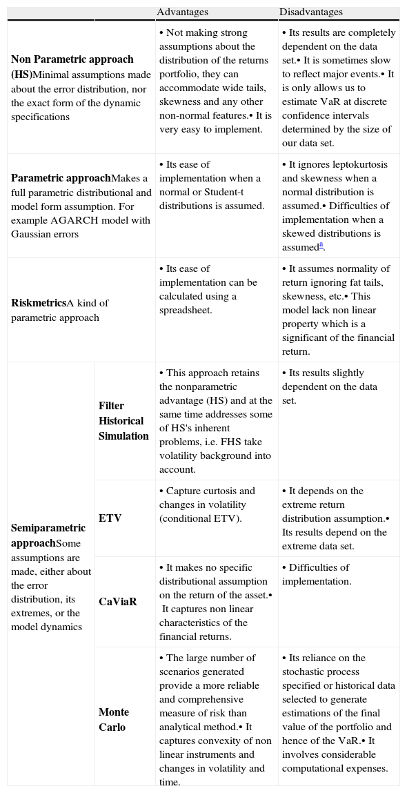
To sum up, in this section we have reviewed some of the most important VaR methodologies, from the standard models to the more recent approaches. From a theoretical point of view, all of these approaches show advantages and disadvantages. In Table 3, we resume these advantages and disadvantages. In the next sections, we will review the results obtained for these methodologies from a practical point of view.
Advantages and disadvantages of VaR approaches.
| Advantages | Disadvantages | ||
| Non Parametric approach (HS)Minimal assumptions made about the error distribution, nor the exact form of the dynamic specifications | •Not making strong assumptions about the distribution of the returns portfolio, they can accommodate wide tails, skewness and any other non-normal features.•It is very easy to implement. | •Its results are completely dependent on the data set.•It is sometimes slow to reflect major events.•It is only allows us to estimate VaR at discrete confidence intervals determined by the size of our data set. | |
| Parametric approachMakes a full parametric distributional and model form assumption. For example AGARCH model with Gaussian errors | •Its ease of implementation when a normal or Student-t distributions is assumed. | •It ignores leptokurtosis and skewness when a normal distribution is assumed.•Difficulties of implementation when a skewed distributions is assumeda. | |
| RiskmetricsA kind of parametric approach | •Its ease of implementation can be calculated using a spreadsheet. | •It assumes normality of return ignoring fat tails, skewness, etc.•This model lack non linear property which is a significant of the financial return. | |
| Semiparametric approachSome assumptions are made, either about the error distribution, its extremes, or the model dynamics | Filter Historical Simulation | •This approach retains the nonparametric advantage (HS) and at the same time addresses some of HS's inherent problems, i.e. FHS take volatility background into account. | •Its results slightly dependent on the data set. |
| ETV | •Capture curtosis and changes in volatility (conditional ETV). | •It depends on the extreme return distribution assumption.•Its results depend on the extreme data set. | |
| CaViaR | •It makes no specific distributional assumption on the return of the asset.•It captures non linear characteristics of the financial returns. | •Difficulties of implementation. | |
| Monte Carlo | •The large number of scenarios generated provide a more reliable and comprehensive measure of risk than analytical method.•It captures convexity of non linear instruments and changes in volatility and time. | •Its reliance on the stochastic process specified or historical data selected to generate estimations of the final value of the portfolio and hence of the VaR.•It involves considerable computational expenses. | |
In addition, as the skewness distributions are not included in any statistical package, the user of this methodology have to program their code of estimation To do that, several program language can be used: MATLAB, R, GAUSS, etc. It is in this sense we say that the implementation is difficult. As the maximisation of the likelihood based on several skewed distributions, such as, SGT is very complicated so that it can take a lot of computational time.
Many authors are concerned about the adequacy of the VaR measures, especially when they compare several methods. Papers, which compare the VaR methodologies commonly use two alternative approaches: the basis of the statistical accuracy tests and/or loss functions. As to the first approach, several procedures based on statistical hypothesis testing have been proposed in the literature and authors usually select one or more tests to evaluate the accuracy of VaR models and compare them. The standard tests about the accuracy VaR models are: (i) unconditional and conditional coverage tests; (ii) the back-testing criterion and (iii) the dynamic quantile test. To implement all these tests an exception indicator must be defined. This indicator is calculated as follows:

Kupiec (1995) shows that assuming the probability of an exception is constant, then the number of exceptions x=∑It+1 follows a binomial distribution B(N, α), where N is the number of observations. An accurate VaR(α) measure should produce an unconditional coverage(αˆ=∑It+1/N) equal to α percent. The unconditional coverage test has as a null hypothesis αˆ=α, with a likelihood ratio statistic:
which follows an asymptotic χ2(1) distribution.
Christoffersen (1998) developed a conditional coverage test. This jointly examines whether the percentage of exceptions is statistically equal to the one expected and the serial independence of It+1. He proposed an independence test, which aimed to reject VaR models with clustered violations. The likelihood ratio statistic of the conditional coverage test is LRcc=LRuc+LRind, which is asymptotically distributed χ2(2), and the LRind statistic is the likelihood ratio statistic for the hypothesis of serial independence against first-order Markov dependence.10
A similar test for the significance of the departure of αˆ from α is the back-testing criterion statistic:
which follows an asymptotic N(0,1) distribution.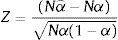
Finally, the Dynamic Quantile (DQ) test proposed by Engle and Manganelli (2004) examines whether the exception indicator is uncorrelated with any variable that belongs to the information set Ωt−1 available when the VaR was calculated. This is a Wald test of the hypothesis that all slopes in the regression model
are equal to zero, where Xj are explanatory variables contained in Ωt−1.VaR(α) is usually an explanatory variable to test if the probability of an exception depends on the level of the VaR.
The tests described above are based on the assumption that the parameters of the models fitted to estimate the VaR are known, although they are estimations. Escanciano and Olmo (2010) show that the use of standard unconditional and independence backtesting procedures can be misleading. They propose a correction of the standard backtesting procedures. Additionally, Escanciano and Pei (2012) propose correction when VaR is estimated with HS or FHS. On a different route, Baysal and Staum (2008) provide a test on the coverage of confidence regions and intervals involving VaR and Conditional VaR.
The second approach is based on the comparison of loss functions. Some authors compare the VaR methodologies by evaluating the magnitude of the losses experienced when an exception occurs in the models. The “magnitude loss function” that addresses the magnitude of the exceptions was developed by Lopez (1998, 1999). It deals with a specific concern expressed by the Basel Committee on Banking Supervision, which noted that the magnitude, as well as the number of VaR exceptions is a matter of regulatory concern. Furthermore, the loss function usually examines the distance between the observed returns and the forecasted VaR(α) values if an exception occurs.
Lopez (1999) proposed different loss functions:
where the VaR measure is penalised with the exception indicator (z(.)=1), the exception indicator plus the square distance (z(.)=1+(rt+1−VaR(α))2 or using weight (z(rt+1,VaR(α)x)=k, where x, being the number of exceptions, is divided into several zones and k is a constant which depends on zone) based on what regulators consider to be a minimum capital requirement reflecting their concerns regarding prudent capital standards and model accuracy.
More recently, other authors have proposed loss function alternatives, such as Abad and Benito (2013) who consider z(.)=(rt+1−VaR(α))2and z(.)=|rt+1−VaR(α)| or Caporin (2008) who proposes z(.)=1−rt+1/VaR(α) and z(.)=((|rt+1|−|VaR(α)|)2/|VaR(α)|). Caporin (2008) also designs a measure of the opportunity cost.
In this second approach, the best VaR model is that which minimises the loss function. In order to know which approach provides minimum losses, different tests can be used. For instance Abad and Benito (2013) use a non-parametric test while Sener et al. (2012) use the Diebold and Mariano (1995) test as well as that of White (2000).
Another alternative to compare VaR models is to evaluate the loss in a set of hypothetical extreme market scenarios (stress testing). Linsmeier and Pearson (2000) discuss the advantages of stress testing.
4Comparison of VaR methodsEmpirical literature on VaR methodology is quite extensive. However, there are not many papers dedicated to comparing the performance of a large range of VaR methodologies. In Table 4, we resume 24 comparison papers. Basically, the methodologies compared in these papers are HS (16 papers), FHS (8 papers), the Parametric method under different distributions (22 papers included the normal, 13 papers include t-Student and just 5 papers include any kind of skewness distribution) and the EVT based approach (18 papers). Only a few of these studies include other methods, such as the Monte Carlo (5 papers), CaViaR (5 papers) and the Non-Parametric density estimation methods (2 papers) in their comparisons. For each article, we marked the methods included in the comparative exercise with a cross and shaded the method that provides the best VaR estimations.
Overview of papers that compare VaR methodologies: what methodologies compare?
| HS | FHS | RM | Parametric approaches | ETV | CF | CaViaR | MC | N-P | |||||
| N | T | SSD | MN | HOM | |||||||||
| Abad and Benito (2013) | × | × | × | × | × | × | |||||||
| Gerlach et al. (2011) | × | × | × | × | |||||||||
| Sener et al. (2012) | × | × | × | × | × | × | |||||||
| Ergun and Jun (2010) | × | × | × | × | × | ||||||||
| Nozari et al. (2010) | × | × | |||||||||||
| Polanski and Stoja (2010) | × | × | × | × | × | × | |||||||
| Brownlees and Gallo (2010) | × | × | × | × | |||||||||
| Yu et al. (2010) | × | × | × | × | |||||||||
| Ozun et al. (2010) | × | × | × | × | |||||||||
| Huang (2009) | × | × | × | × | |||||||||
| Marimoutou et al. (2009) | × | × | × | × | |||||||||
| Zikovic and Aktan (2009) | × | × | × | × | |||||||||
| Giamouridis and Ntoula (2009) | × | × | × | × | × | ||||||||
| Angelidis et al. (2007) | × | × | × | × | × | ||||||||
| Tolikas et al. (2007) | × | × | × | × | |||||||||
| Alonso and Arcos (2006) | × | × | × | × | |||||||||
| Bao et al. (2006) | × | × | × | × | × | × | × | ||||||
| Bhattacharyya and Ritolia (2008) | × | × | × | ||||||||||
| Kuester et al. (2006) | × | × | × | × | × | × | × | ||||||
| Bekiros and Georgoutsos (2005) | × | × | × | × | × | ||||||||
| Gençay and Selçuk (2004) | × | × | × | × | |||||||||
| Gençay et al. (2003) | × | × | × | × | |||||||||
| Darbha (2001) | × | × | × | ||||||||||
| Danielsson and de Vries (2000) | × | × | × | × | |||||||||
Note: In this table, we present some empirical papers involving comparisons of VaR methodologies. The VaR methodologies are marked with a cross when they are included in a paper. A shaded cell indicates the best methodology to estimate the VaR in the paper. The VaR approaches included in these paper are the following: Historical Simulation (HS); Filtered Historical Simulation (FHS); Riskmetrics (RM); Parametric approaches estimated under different distributions, including the normal distribution (N), t-Student distribution (T), skewed t-Student distribution (SSD), mixed normal distribution (MN) and high-order moment time-varying distribution (HOM); Extreme Value Theory (EVT); CaViaR method (CaViaR); Monte Carlo Simulation (MC); and non-parametric estimation of the density function (N–P).
The approach based on the EVT is the best for estimating the VaR in 83.3% of the cases in which this method is included in the comparison, followed closely by FHS, with 62.5% of the cases. This percentage increases to 75.0% if we consider that the differences between ETV and FHS are almost imperceptible in the paper of Giamouridis and Ntoula (2009), as the authors underline. The CaViaR method ranks third. This approach is the best in 3 out of 5 comparison papers (it represents a percentage of success of 60%, which is quite high). However, we must remark that only in one of these 3 papers, ETV is included in the comparison and FHS is not included in any of them.
The worst results are obtained by HS, Monte Carlo and Riskmetrics. None of those methodologies rank best in the comparisons where they are included. Furthermore, in many of these papers HS and Riskmetrics perform worst in estimating VaR. A similar percentage of success is obtained by Parametric method under a normal distribution. Only in 2 out of 18 papers, does this methodology rank best in the comparison. It seems clear that the new proposals to estimate VaR have outperformed the traditional ones.
Taking this into account, we highlight the results obtained by Berkowitz and O’Brien (2002). In this paper the authors compare some internal VaR models used by banks with a parametric GARCH model estimated under normality. They find that the bank VaR models are not better than a simple parametric GARCH model. It reveals that internal models work very poorly in estimating VaR.
The results obtained by the Parametric method should be taken into account when the conditional high-order moments are time-varying. The two papers that include this method in the comparison obtained a 100% outcome success (see Ergun and Jun, 2010; Polanski and Stoja, 2010). However, only one of these papers included EVT in the comparison (Ergun and Jun, 2010).
Although not shown in Table 4, the VaR estimations obtained by the Parametric method with asymmetric and leptokurtic distributions and in a mixed-distribution context are also quite accurate (see Abad and Benito, 2013; Bali and Theodossiou, 2007, 2008; Bali et al., 2008; Chen et al., 2011; Polanski and Stoja, 2010). However this method does not seem to be superior to EVT and FHS (Kuester et al., 2006; Cifter and Özün, 2007; Angelidis et al., 2007). Nevertheless, there are not many papers including these three methods in their comparison. In this line, some recent extensions of the CaViaR method seem to perform quite well, such as those proposed by Yu et al. (2010) and Gerlach et al. (2011). This last paper compared three CAViaR models (SAV, AS and Threshold CAViaR) with the Parametric model under some distributions (GARCH-N, GARCH-t, GJR-GARCH, IGARCH, Riskmetric). They find that at 1% confidence level, the Threshold CAViaR model performs better than the Parametric models considered. Sener et al. (2012) carried out a comparison of a large set of VaR methodologies: HS, Monte Carlo, EVT, Riskmetrics, Parametric method under normal distribution and four CaViaR models (symmetric and asymmetric). They find that the asymmetric CaViaR model joined to the Parametric model with an EGARCH model for the volatility performs the best in estimating VaR. Abad and Benito (2013), in a comparison of a large range of VaR approaches that include EVT, find that the Parametric method under an asymmetric specification for conditional volatility and t-Student innovations performs the best in forecasting VaR. Both papers highlight the importance of capturing the asymmetry in volatility. Sener et al. (2012) state that the performance of VaR methods does not depend entirely on whether they are parametric, non-parametric, semi-parametric or hybrid but rather on whether they can model the asymmetry of the underlying data effectively or not.
In Table 5, we reconsider the papers of Table 4 to show which approach they use to compare VaR models. Most of the papers (62%) evaluate the performance of VaR models on the basis of the forecasting accuracy. To do that not all of them used a statistical test. There is a significant percentage (25%) comparing the percentage of exceptions with that expected without using any statistical test. 38% of the papers in our sample consider that both the number of exceptions and their size are important and include both dimensions in their comparison.
Overview of papers that compare VaR methodologies: how do they compare?
| The accuracy | Loss function | |
| Abad and Benito (2013) | LRuc-ind-cc, BT, DQ | Quadratic |
| Gerlach et al. (2011) | LRuc-cc, DQ | |
| Sener et al. (2012) | DQ | Absolute |
| Ergun and Jun (2010) | LRuc-ind-cc | |
| Nozari et al. (2010) | LRuc | |
| Polanski and Stoja (2010) | LRuc-ind | |
| Brownlees and Gallo (2010) | LRuc-ind-cc, DQ | Tick loss function |
| Yu et al. (2010) | % | |
| Ozun et al. (2010) | LRuc-ind-cc | Quadratic's Lopez |
| Huang (2009) | LRuc | |
| Marimoutou et al. (2009) | LRuc-cc | Quadratic's Lopez |
| Zikovic and Aktan (2009) | LRuc-ind-cc | Lopez |
| Giamouridis and Ntoula (2009) | LRuc-ind-cc | |
| Angelidis et al. (2007) | LRuc | Quadratic |
| Tolikas et al. (2007) | LRcc | |
| Alonso and Arcos (2006) | BT | Quadratic's Lopez |
| Bao et al. (2006) | % | Predictive quantile loss |
| Bhattacharyya and Ritolia (2008) | LRuc | |
| Kuester et al. (2006) | LRuc-ind-cc, DQ | |
| Bekiros and Georgoutsos (2005) | LRuc-cc | |
| Gençay and Selçuk (2004) | % | |
| Gençay et al. (2003) | % | |
| Darbha (2001) | % | |
| Danielsson and de Vries (2000) | % |
Note: In this table, we present some empirical papers involving comparisons of VaR methodologies. We indicate the test to evaluate the accuracy of VaR models and/or the loss function used in the comparative exercise. LRuc is the unconditional coverage test. LRind is the statistic for the serial independence. LRcc is the conditional coverage test. BT is the back-testing criterion. DQ is the Dynamic Quantile test. % denotes the comparison of the percentage of exceptions with the expected percentage without a statistical test.
Although there are not many articles dedicated to the comparison of a wide range of VaR methodologies, the existing ones offer quite conclusive results. These results show that the approach based on the EVT and FHS is the best method to estimate the VaR. We also note that VaR estimates obtained by some asymmetric extensions of CaViaR method and the Parametric method under the skewed and fat-tail distributions lead to promising results, especially when the assumption that the standardised returns is iid is abandoned and the conditional high-order moments are considered to be time-varying.
5Some important topics of VaR methodologyAs we stated in the introduction, VaR is by far the leading measure of portfolio risk in use in major commercial banks and financial institutions. However, this measurement is not exempt from criticism. Some researchers have remarked that VaR is not a coherent market measure (see Artzner et al., 1999). These authors define a set of criteria necessary for what they call a “coherent” risk measurement. These criteria include homogeneity (larger positions are associated with greater risk), monotonicity (if a portfolio has systematically lower returns than another for all states of the world, its risk must be greater), subadditivity (the risk of the sum cannot be greater than the sum of the risk) and the risk free condition (as the proportion of the portfolio invested in the risk free asset increases, portfolio risk should decline). They show that VaR is not a coherent risk measure because it violates one of their axioms. In particular VaR does not satisfy the subadditivity condition and it may discourage diversification. On this point Artzner et al. (1999) proposed an alternative risk measure related to VaR which is called Tail Conditional Expection, also called Conditional Value at Risk (CVaR). The CVaR measures the expected loss in the α% worst cases and is given by
The CVaR is a coherent measure of risk when it is restricted to continuous distributions. However, it can violate sub-additivity with non-continuous distributions. Consequently, Acerbi and Tasche (2002) proposed the Expected Shortfall (ES) as a coherent measure of risk. The ES is given by
where λ≡(Pt−1[Rt≤−VaRtα]/α)≥1. Note that CVaR=ES when the distribution of returns is continuous. However, it is still coherent when the distribution of returns is not continuous. The ES has also several advantages when compared with the more popular VaR. First of all, the ES is free of tail risk in the sense that it takes into account information about the tail of the underlying distribution. The use of a risk measure free of tail risk avoids extreme losses in the tail. Therefore, the ES is an excellent candidate for replacing VaR for financial risk management purposes.
Despite the advantages of ES, it is still less used than VaR. The principal reason for this pretermission is that the ES backtest is harder than VaR one. In that sense, in the last years some ES backtesting procedures have been developed. We can cite here the residual approach introduced by McNeil and Frey (2000), the censored Gaussian approach proposed by Berkowitz (2001), the functional delta approach of Kerkhof and Melenberg (2004), and the saddlepoint technique introduced by Wong (2008, 2010).
However, these approaches present some drawbacks. The backtests of McNeil and Frey (2000), Berkowitz (2001) and Kerkhof and Melenberg (2004) rely on asymptotic test statistics that might be inaccurate when the sample size is small. The test proposed by Wong (2008) is robust to these questions; nonetheless, it has some disadvantages (as with the Gaussian distribution assumption).
Regardless of the sector in which a financial institution participates, all such institutions are subject to three types of risk: market, credit and operational. So, to calculate the total VaR of a portfolio it is necessary to combine these risks. There are different approximations to carry this out. First, an approximation that sums up the three types of risk (VaR). As VaR is not a subadditivity measure this approximation overestimates total risk or economic capital. Second, assuming joint normality of the risk factors, this approximation imposes tails that are thinner than the empirical estimates and significantly underestimates economic capital and the third approach to assess the risk aggregation is based on using copulas. To obtain the total VaR of a portfolio it is necessary to obtain the joint return distribution of the portfolio. Copulas allow us to solve this problem by combining the specific marginal distributions with a dependence function to create this joint distribution. The essential idea of the copula approach is that a joint distribution can be factored into the marginals and a dependence function, called copula. The term copula is based on the notion of coupling: the copula couples the marginal distributions together to form a joint distribution. The dependence relation is entirely determined by the copula, while location, scaling and shape are entirely determined by the marginals. Using a copula, marginal risk that is initially estimated separately can then be combined in a joint risk distribution preserving the marginals original characteristics. This is sometimes referred to as obtaining a joint density with predetermined marginals. The joint distribution can then be used to calculate the quantiles of the portfolio return distribution, since the portfolio returns are a weighted average on individual returns. Embrechts et al. (1999, 2002) were among the first to introduce this methodology in financial literature. Some applications of copulas focussing on cross-risk aggregation for financial institutions can be found in Alexander and Pezier (2003), Ward and Lee (2002) and Rosenberg and Schuermann (2006).
6ConclusionIn this article we review the full range of methodologies developed to estimate the VaR, from standard models to the recently proposed and present their relative strengths and weaknesses from both theoretical and practical perspectives.
The performance of the parametric approach in estimating the VaR depends on the assumed distribution of the financial return and on the volatility model used to estimate the conditional volatility of the returns. As for the return distribution, empirical evidence suggests that when asymmetric and fat-tail distributions are considered, the VaR estimate improves considerably. Regardless of the volatility model used, the results obtained in the empirical literature indicate the following: (i) The EWMA model provides inaccurate VaR estimates, (ii) the performance of the GARCH models strongly depends on the assumption of returns distribution. Overall, under a normal distribution, the VaR estimates are not very accurate, but when asymmetric and fat-tail distributions are applied, the results improve considerably, (iii) evidence suggests with some exceptions that SV models do not improve the results obtained by the family of GARCH models, (iv) the models based on the realised volatility work quite well to estimate VaR, outperforming the GARCH models estimated under a normal distribution. Additionally, Markov-Switching GARCH outperforms the GARCH models estimated under normality. In the case of the realised volatility models, some authors indicate that its superiority compared with the GARCH family is not as high when the GARCH models are estimated assuming asymmetric and fat-tail returns distributions, (v) in the GARCH family, the fractional-integrated GARCH models do not appear to be superior to the GARCH models. However, in the context of the realised volatility models, there is evidence that models, which capture long memory in volatility, provide more accurate VaR estimates, and (vi) although evidence is somewhat ambiguous, asymmetric volatility models appear to provide a better VaR estimate than symmetric models.
Although there are not many works dedicated to the comparison of a wide range of VaR methodologies, the existing ones offer quite conclusive results. These results show that the approach based on the EVT and FHS is the best method to estimate the VaR. We also note that VaR estimates obtained by some asymmetric extension of CaViaR method and the Parametric method under the skewed and fat-tail distributions lead to promising results, especially when the assumption that the standardised returns is iid is abandoned and that the conditional high-order moments are considered to be time-varying. It seems clear that the new proposals to estimate VaR have outperformed the traditional ones.
To further the research, it would be interesting to explore whether in the context of an approach based on the EVT and FHS considering asymmetric and fat-tail distributions to model the volatility of the returns could help to improve the results obtained by these methods. Along this line, results may be further improved by applying the realised volatility model and Markov-switching model.
This work has been funded by the Spanish Ministerio de Ciencia y Tecnología (ECO2009-10398/ECON and ECO2011-23959).
When the Basel I Accord was concluded in 1988, no capital requirement was defined for the market risk. However, regulators soon recognised the risk to a banking system if insufficient capital was held to absorb the large sudden losses from huge exposures in capital markets. During the mid-90s, proposals were tabled for an amendment to the 1988 accord, requiring additional capital over and above the minimum required for credit risk. Finally, a market risk capital adequacy framework was adopted in 1995 for implementation in 1998. The 1995 Basel I Accord amendment provided a menu of approaches for determining the market risk capital requirements.
There is another market risk measurement, called Expected Shortfall (ES). ES measures the expected value of our losses if we get a loss in excess of VaR. So that, this measure tells us what to expect in a bad estate, while the VaR tells us nothing more than to expect a loss higher than the VaR itself. In Section 5, we will formally define this measure besides presenting some criticisms of VaR measurement.
For a more pedagogic review of some of these methodologies (see Feria Domínguez, 2005).
Thus, if we have, e.g., 100 observations, it allows us to estimate VaR at the 95% confidence level but not the VaR at the 95.1% confidence level. The VaR at the 95% confidence level is given by the sixth largest loss, but the VaR at the 95.1% confidence level is a problem because there is no loss observation to accompany it.
The EWMA model is equivalent to the IGARCH model with the intercept α0 being restricted to being zero, the autoregressive parameter β being set at a pre-specific value λ, and the coefficient of εt−12 being equal to 1−λ.
This last paper shows that t-Student at 1% performs better in larger positions, although it does not in short positions.
Although in different contexts, approximating the distribution of asset returns via the GCE has been previously employed in the literature (e.g., Jarrow and Rudd, 1982; Baillie and Bollerslev, 1992; Jondeau and Rockinger, 2001; Leon et al., 2005; Christoffersen and Diebold, 2006).
To estimate the volatility of the returns, several volatility models can be used. Hull and White (1998) proposed a GARCH model and the EWMA model.
The LRind statistic is LRind=2 [logLA−logL0] and has an asymptotic χ2(1) distribution. The likelihood function under the alternative hypothesis is LA=(1−π01)N00π01N01(1−π11)N10π11N11 where Nij denotes the number of observations in state j after having been in state i in the previous period, π01=N01/(N00+N01) and π11=N11/(N10+N11). The likelihood function under the null hypothesis is (π01=π11=π=(N11+N01)/N) is L0=(1−π)N00+N01πN01+N11.

