Multivariate GARCH models and risk minimizing portfolios: The importance of medium and small firms

Abstract

This paper re-examines the relationship among different firms using a combination of multivariate GARCH models (symmetric and asymmetric with structural changes) and the IBEX 35, IBEX MEDIUM CAP, and IBEX SMALL CAP indexes as the benchmarks to track the performance of large, medium and small firms, respectively. Our findings show the existence of a significant difference in the transmission of volatility when the asymmetric behavior and structural changes are considered. After calculating the risk minimizing portfolio weights, we show that the minimum-volatility portfolio is composed of medium and small indexes with a higher weight of medium firms for a set of different scenarios.

1

Introduction

The strong performance of medium and small firms has inspired huge interest among investors, analysts, financial intermediaries, communication media, and financial market participants in general during the last few years. Some interesting studies are those of Ewing and Malik (2005) and Hassan and Malik (2007), where the relationships between large and small firms in the US market are analyzed, or those of Aragó and Fernández (2007) and Pardo and Torró (2007) who analyzed that relationship for the Spanish stock markets.

The present paper re-examines the relationship among different firms using the IBEX 35, IBEX MEDIUM CAP, and IBEX SMALL CAP indexes as the benchmarks to track the performance of large, medium and small firms, respectively.¹ This study emphasizes to the role that sudden changes in variance may play not only in the transmission process but also in the calculation of risk minimizing portfolios.

We improve the previous literature in various ways. Firstly, to our knowledge this paper is the first one to focus on all three IBEX indexes. Pardo and Torró (2007) and Chuliá and Torró (2007) used the Ibex Complementario and the Ibex Medium Cap taking them as the reference for the small firms. Secondly, in order to check the robustness of our results, we employ a symmetric and an asymmetric multivariate GARCH model with structural changes. Thirdly, since different assets are traded based on these indexes, we use the estimated volatilities to calculate the risk minimizing portfolio weights considering the methodology of Kroner and Ng (1998) and a set of different scenarios. Finally, we shed some light on the behavior of the Spanish stock market by providing some clues to better understand portfolio allocations.

Our study focuses on the Spanish stock market because in recent years it has become a reference for the main European stock markets due to improvements in the technical, operational and organizational systems supporting the market which have enabled it to channel large volumes of investment and have made it more transparent, liquid, and effective.

Our findings show the existence of a significant difference in the transmission of volatility when asymmetric behavior and structural changes are considered. However, the most interesting results are related to the risk minimizing portfolio composition. For all the different scenarios analyzed, we show that the minimum-volatility portfolio is composed of medium and small indexes with a higher weight of medium firms. These results have important implications for building accurate asset pricing models, forecasting volatility, and understanding the Spanish stock market.

The remainder of the paper is organized as follows: Section 2 presents a review of related literature. Section 3 describes the data and methodology. In Section 4 we show the principal results and, finally, in Section 5 we provide the main conclusions.

2

Literature review

One of the most important issues in finance in recent years has been the analysis of price and volatility spillovers among stock markets, sector indexes, or small and large firm portfolios. Initial studies such as those by Hamao et al. (1990), King and Wadhwani (1990) and Lin et al. (1994), among others, were followed by others such as Fleming et al. (1998), who demonstrated how cross market hedging and sharing of common information could lead to transmission of volatility across markets over time, or those of Chelley-Steeley and Steeley (1996) and Grieb and Reyes (2002), who examine data for the UK using different methodologies and show the existence of a bi-directional feedback of conditional variances between UK firms of different sizes.

More recently, Malik and Hammoudeh (2007) analyze the volatility and shock transmission mechanism among equity and global crude oil markets of US and Gulf countries. Ewing and Malik (2005) examine the asymmetry in the predictability of volatility allowing for sudden changes in variance by using the Bivariate GARCH model. Finally, Hassan and Malik (2007) and Li and Majerowska (2008) use multivariate GARCH models (including more than two variables) to analyze the transmission of shocks and volatility among different US sector indexes and links between emerging stock markets in Poland and Hungary and established markets in Germany and the US, respectively.

Volatility behavior in the Spanish stock market has also been studied in recent years. Cuñado et al. (2004) analyze the behavior of volatility in the Spanish stock market by detecting if volatility has changed its behavior significantly over a period and by identifying the causes. The results show that the Spanish stock market is subject to higher, but less persistent, volatility and that trading volume significantly impacts on volatility.

Aragó and Fernández (2007) analyze the European transmission of information through volatilities with structural changes in variance for the main stock indexes following the ICSS algorithm to detect sudden changes. Their findings suggest that markets react not only to local news, but also to news originating in other markets, especially adverse news. Soriano and Climent (2006a) use a multivariate GARCH approach to analyze the importance of regional versus industrial effects and volatility transmission patterns in a particular industry across different regions. Chuliá and Torró (2007) analyze volatility spillovers between large and small firms in the Spanish stock market by using a conditional CAPM with an asymmetric multivariate GARCH-M model.

Finally, Pardo and Torró (2007) study volatility spillovers between large and small firms by analyzing the impulse-response function for conditional volatility computed following the Lin (1997), and Meneu and Torró (2003) procedure. They show that volatility spillovers exist in both directions between those portfolios after bad news.

This paper adds a new point of view to the analysis of volatility in the Spanish stock market. As opposed to the previous empirical evidence, we focus on large, medium and small firms and propose a risk minimizing portfolio strategy based on a multivariate GARCH methodology. Additionally, in order to obtain more conclusive economic implications, we analyze the optimal portfolio responses to good and bad news.

3

Data and methodology

3.1

Data

The data consists of daily close returns (calculated as logarithmic differences) for the IBEX 35, IBEX MEDIUM CAP, and IBEX SMALL CAP indexes for the period from January 14, 1992 to December 30, 2011.²

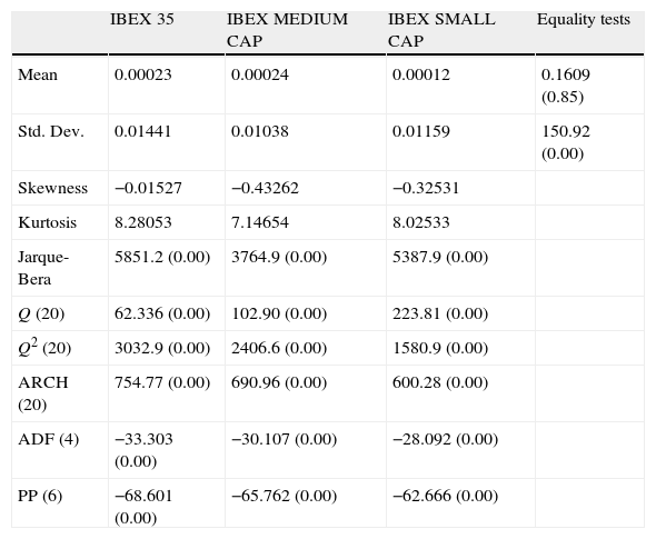
Table 1 presents the summary statistics for these return series. An initial conclusion might suggest that the performance of the IBEX MEDIUM CAP as measured by mean return is better (0.024%) than the IBEX 35 (0.023%) and the IBEX SMALL CAP (0.012%). However, on the basis of the Anova test we cannot reject the null hypothesis that all series in the group have the same mean since those differences are not statistically significant. On the other hand, due to the rejection of the null hypothesis of equality of variances among the return series, we can conclude that the IBEX MEDIUM CAP index is less volatile (standard deviation of 1.03%) than the other two indexes (1.15% and 1.44% for IBEX SMALL CAP and IBEX 35, respectively). These preliminary results are consistent with those obtained previously by Pardo and Torró (2007) and Chuliá and Torró (2007) for large and small Spanish indexes and point out that it is important to study more accurately the covariance dynamics among these indexes.

Table 1.

Descriptive statistics.

	IBEX 35	IBEX MEDIUM CAP	IBEX SMALL CAP	Equality tests
Mean	0.00023	0.00024	0.00012	0.1609 (0.85)
Std. Dev.	0.01441	0.01038	0.01159	150.92 (0.00)
Skewness	−0.01527	−0.43262	−0.32531
Kurtosis	8.28053	7.14654	8.02533
Jarque-Bera	5851.2 (0.00)	3764.9 (0.00)	5387.9 (0.00)
Q (20)	62.336 (0.00)	102.90 (0.00)	223.81 (0.00)
Q^2 (20)	3032.9 (0.00)	2406.6 (0.00)	1580.9 (0.00)
ARCH (20)	754.77 (0.00)	690.96 (0.00)	600.28 (0.00)
ADF (4)	−33.303 (0.00)	−30.107 (0.00)	−28.092 (0.00)
PP (6)	−68.601 (0.00)	−65.762 (0.00)	−62.666 (0.00)

This table presents descriptive statistics for the daily return series of the Ibex 35, the Ibex Medium Cap and the Ibex Small Cap indexes. Last column reports the mean and variance equality tests using the ANOVA and Levene statistics, respectively. Skewness and Kurtosis refer to the series skewness and kurtosis coefficients. The Jarque-Bera statistic tests the normality of the series. This statistic has an asymptotic χ² (2) distribution under the normal distribution hypothesis. Q (20) and Q² (20) are Ljung–Box tests for 20th-order serial correlation in the returns and squared returns. ARCH (20) is the Engle (1982) test for the 20th-order ARCH. These three tests are distributed as χ² (20). The ADF (4) and PP (6) refer to the Augmented Dickey and Fuller (1981) and Phillips and Perron (1988) unit root tests corresponding to the process with intercept but without trend. The p-values of these tests are reported in parenthesis.

Further test produce similar results for these three series. Skewness and kurtosis values indicate that the distributions of returns for all the indexes are negatively skewed and leptokurtic. The Jarque-Bera statistic rejects the null hypothesis that the returns are normally distributed for all cases.³ The Ljung-Box statistic for up to 20 lags indicates the presence of significant linear and non-linear dependencies in the returns of all indexes. The ARCH test reveals that returns exhibit conditional heteroskedasticity and the augmented Dickey and Fuller and Philips and Perron tests indicate that these time series are stationary.

Finally, in order to illustrate the evolution of the three indexes, we show their charts for the period analyzed in Fig. 1. We can clearly observe some significant trends (upwards and downwards) in the medium and small firm indexes in contrast to the more volatile behavior of the IBEX 35 in which these trends are repeated during the period.

Fig. 1.

Performance of the stock indexes IBEX 35, IBEX MEDIUM CAP and IBEX SMALL CAP.

3.2

Methodology

On the basis of the features observed in the previous section, GARCH models will be appropriate. As the initial aim of this study is to re-examine the volatility transmission of large, medium, and small value firm portfolios in the Spanish stock market, we will use a trivariate GARCH model.

The first step in the trivariate GARCH procedure is to identify the best-fitting specification of the return series. This is particularly important as mis-specifying the mean equation may lead to an incorrect estimation of the variance equation (Ewing and Malik, 2005). Once the mean structure is identified, we estimate the mean and variance specifications jointly to avoid the generated regressor problem (according to Ewing et al., 2002).

Therefore, the conditional mean equations are defined as a VAR(15) process⁴:

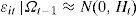
where R_1,t, R_2,t and R_3,t are the daily returns for the Ibex-35, Ibex medium cap and Ibex small cap indexes, respectively, c_i and α_ij for i = 1, 2, and 3, and j = 1, 2, and 3 are the parameters to be estimated, ε_it indicates the innovations for each index at time t following a normal distribution with a mean of 0 and variance H_t where Ω_t−1 is the information set in t − 1. The VAR lag has been chosen following the Akaike information criterion.⁵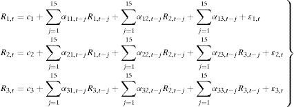

We employ the BEKK representation, introduced by Baba et al. (1991), to model the conditional variance-covariance matrix⁶:

where, in our case, C is a (3 × 3) lower triangular matrix with six parameters and A and B are squared (3 × 3) matrices of parameters. The elements of A capture the effects of shocks or events on volatility while the elements of B capture the effects of past conditional variances measuring the diagonal parameters the effects of own past shocks and past volatility in both cases. The total number of estimated elements for the variance equations in our trivariate case is 24.

where

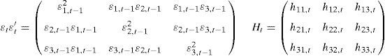
Without using matrices we get the following forms for the conditional variances,

However, previous studies document the relevance of considering structural changes in variance and asymmetries, which are the different responses of volatility to negative shocks (bad news) or positive shocks (good news). More precisely, Pardo and Torró (2007) and Chuliá and Torró (2007) propose an asymmetric bivariate GARCH model to analyze volatility spillovers between large and small firms in the Spanish stock market. However, they do not incorporate the role of sudden changes in volatility as proposed by Ewing and Malik (2005), Aragó and Fernández (2007) and Aragó and Salvador (2011). Based on these previous studies, we extend the latter model to allow for both aspects.

The methodology used in this study to identify sudden shifts in the variance of an observed time series is based on the ICSS algorithm developed by Inclan and Tiao (1994), and used by Aggarwal et al. (1999), Malik (2003), and Ewing and Malik (2005).

The analysis assumes that the time series exhibit a stationary variance over an initial period until a sudden change in variance occurs. The variance is then stationary again for a time until the next sudden change. The process is repeated over time, yielding a time series of observations with an unknown number of changes in the variance.

Let ε_t be a series with zero mean and with unconditional variance σt2. Let the variance within each interval be given by σj2, j = 0, 1, …, N_T where N_T is the total number of variance changes in T observations and 1<κ1<κ2<…<κNT

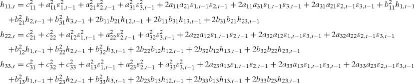
A cumulative sum of squares is used to estimate the number of changes in variance and the point in time of each variance shift. Let Ck=∑t=1kϵt2, k=1,…,T, be the cumulative sum of the squared observations from the start of the series to the k-th point in time, where k is a point of sudden change and T is the number of observations. The D_k statistic is defined as follows:

where C_T is the sum of the squared residuals from the whole sample period.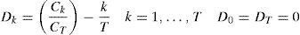

If there are no changes in variance over the sample period, the D_k statistic oscillates around zero (a horizontal line when plotted against k). However, if the series contains variance changes, the D_k values drift either above or below zero. Critical values based on the distribution of D_k under the null hypothesis of homogeneous variance provide upper and lower boundaries to detect a significant change in variance with a known level of probability. In this way, the null hypothesis of constant variance is rejected if the maximum absolute value of D_k is greater than the critical value. So, if maxk(T/2)Dk exceeds the predetermined boundary, then the value of k is taken as an estimate of the change point. The critical value at the 95th percentile is 1.36, therefore upper and lower boundaries can be set at ±1.36 in the D_k plot.

Several recently developed methodologies are available to analyze the asymmetric responses of volatility in variances and covariances: Aragó and Fernández (2007), Chuliá and Torró (2007) and Li and Majerowska (2008). However, in accordance with the subsequent use of the methodology of Kroner and Ng (1998) to compute the optimal portfolio holdings, we employ the extended approach of Glosten et al. (1993) proposed by Kroner and Ng (1998), and also used by Karmakar (2010), to capture the asymmetric effects of news on volatility. The model is specified as:

where I(ϵt−1<0) is a 3 × 1 vector whose elements take value 1 if the corresponding innovation in vector ε_t is negative, and ⊙ is the Hadamard (element by element) product. D is a 3 × 3 diagonal parameters vector; X is a 1 × 3 vector which represents the dummy variables taking a value of 1 from each point of sudden change of variance onwards and zero elsewhere and, finally, n is the number of sudden changes found in each index (three in each case).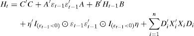

The models are estimated maximizing the likelihood function assuming normally distributed errors:

where T is the number of observations and θ represents the parameter vector to be estimated.⁷

4

Empirical results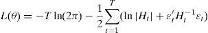

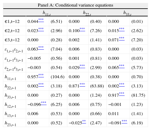
This section presents the empirical results for the models proposed and their economic implications in the calculation of a risk minimizing portfolio strategy. While our initial objective is to model the volatility and shock transmission in large, medium and small firms allowing for asymmetries and structural breaks, it is helpful to first examine the baseline case of the symmetric trivariate GARCH model. The results of estimating this trivariate GARCH model with BEKK parameterization are reported in Table 2.

Table 2.

Trivariate GARCH model.

Panel A: Conditional variance equations
	h11,t		h22,t		h33,t
ϵ1,t−12	0.044^***	(6.51)	0.000	(0.40)	0.000	(0.01)
ϵ2,t−12	0.023^***	(2.96)	0.100^***	(7.26)	0.015^***	(2.62)
ϵ3,t−12	0.000	(0.28)	0.002	(1.41)	0.071^***	(7.20)
ε1,t−1ε2,t−1	0.063^***	(7.04)	0.006	(0.83)	0.000	(0.03)
ε1,t−1ε3,t−1	−0.005	(0.56)	0.001	(0.81)	0.000	(0.03)
ε2,t−1ε3,t−1	−0.003	(0.54)	0.029^***	(2.99)	0.065^***	(5.73)
h11,t−1	0.957^***	(104.6)	0.000	(0.38)	0.000	(0.70)
h22,t−1	0.002^***	(3.18)	0.871^***	(63.88)	0.002^***	(3.13)
h33,t−1	0.000	(0.27)	0.000	(1.24)	0.917^***	(81.75)
h12,t−1	−0.096^***	(6.25)	0.006	(0.75)	−0.001	(1.23)
h13,t−1	0.006	(0.53)	0.000	(0.66)	0.011	(1.41)
h23,t−1	0.000	(0.52)	−0.025^**	(2.47)	−0.091^***	(6.19)

Panel B: Testing restrictions on cross-variance effects
	Chi-squared	(p-value)
H0 : aij = bij ∀ i ≠ j	357.8785	(0.00)
H0 : aij = 0	2885.586	(0.00)
H0 : bij = 0	817848.5	(0.00)

Panel A shows the estimated coefficients of the conditional variance for the large, medium, and small cap return series (the corresponding t-values are given in parenthesis). Panel B reports Wald test of cross-variance effects significance (p-values are reported in parenthesis).

**

Represents the level of significance of 5%.

***

Represents the level of significance of 1%.

Panel A reports the estimated coefficients of the conditional variance for each return series.⁸ We find that conditional variance in large firms (h_11,t) is directly affected by their past news and volatility and directly and indirectly by volatility and news from medium firms. Regarding medium and small firms, we observe that not only are their conditional variances (h_22,t and h_33,t, respectively) directly affected by their own volatility and news, but also by bi-directional transmission of volatility and shocks between each other. This is because both of them are affected directly and indirectly by the news and shocks of the other group of firms. Therefore, each index is closely related with the next one in terms of size, although the relationship between the medium and small firms is closer. Moreover, following Pardo and Torró (2007), we show in Panel B that the null of cross variance effects (a_ij = b_ij ∀ i ≠ j) is clearly rejected as well as the nulls of a_ij = 0 and b_ij = 0. For that reason, we cannot ignore cross relationships across all conditional moments and their symmetric shocks. However, these are preliminary results which do not take into account structural changes in variance and asymmetries.

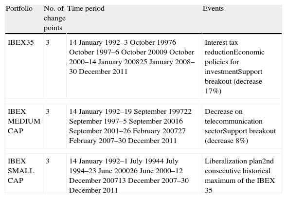
Relative to structural breaks, Table 3 reports the number of sudden changes in volatility detected using the ICSS algorithm. For each index we find three sudden changes which are related with economic policies destined to improve the markets. Additionally, we extend the previous model to allow for the asymmetric responses of volatility in order to measure the effects of negative shocks (bad news) in the variances and to check the robustness of the initial results.

Table 3.

Sudden changes in volatility.

Portfolio	No. of change points	Time period	Events
IBEX35	3	14 January 1992–3 October 19976 October 1997–6 October 20009 October 2000–14 January 200825 January 2008–30 December 2011	Interest tax reductionEconomic policies for investmentSupport breakout (decrease 17%)
IBEX MEDIUM CAP	3	14 January 1992–19 September 199722 September 1997–5 September 20016 September 2001–26 February 200727 February 2007–30 December 2011	Decrease on telecommunication sectorSupport breakout (decrease 8%)
IBEX SMALL CAP	3	14 January 1992–1 July 19944 July 1994–23 June 200026 June 2000–12 December 200713 December 2007–30 December 2011	Liberalization plan2nd consecutive historical maximum of the IBEX 35

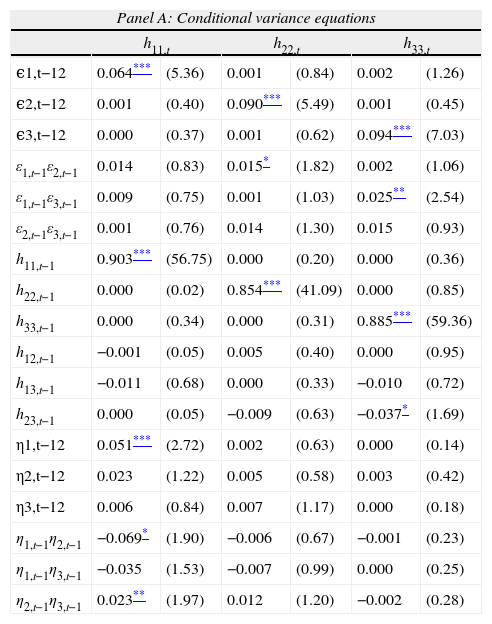
Table 4 reports the most relevant results from the asymmetric trivariate GARCH model with structural changes. Panel A shows the estimated coefficients of the conditional variance equations for each index. As Ewing and Malik (2005) documented for the US market, the significance of these coefficients is quite different from those obtained in the symmetric model (Table 2 Panel A). Relative to the IBEX 35, we observe that now it is affected by its own volatilities and shocks lagged one period and indirectly by medium and small firm shocks. The results from the IBEX MEDIUM CAP are very similar but, in this case, its conditional volatility is also indirectly affected by large firm shocks. Finally, the results related with the small firms show that not only is their conditional volatility directly affected by their own volatility and shocks, but it is also indirectly affected by the shocks and volatility from the IBEX MEDIUM CAP.

Table 4.

Asymmetric trivariate GARCH model with structural changes.

Panel A: Conditional variance equations
	h11,t		h22,t		h33,t
ϵ1,t−12	0.064^***	(5.36)	0.001	(0.84)	0.002	(1.26)
ϵ2,t−12	0.001	(0.40)	0.090^***	(5.49)	0.001	(0.45)
ϵ3,t−12	0.000	(0.37)	0.001	(0.62)	0.094^***	(7.03)
ε1,t−1ε2,t−1	0.014	(0.83)	0.015^*	(1.82)	0.002	(1.06)
ε1,t−1ε3,t−1	0.009	(0.75)	0.001	(1.03)	0.025^**	(2.54)
ε2,t−1ε3,t−1	0.001	(0.76)	0.014	(1.30)	0.015	(0.93)
h11,t−1	0.903^***	(56.75)	0.000	(0.20)	0.000	(0.36)
h22,t−1	0.000	(0.02)	0.854^***	(41.09)	0.000	(0.85)
h33,t−1	0.000	(0.34)	0.000	(0.31)	0.885^***	(59.36)
h12,t−1	−0.001	(0.05)	0.005	(0.40)	0.000	(0.95)
h13,t−1	−0.011	(0.68)	0.000	(0.33)	−0.010	(0.72)
h23,t−1	0.000	(0.05)	−0.009	(0.63)	−0.037^*	(1.69)
η1,t−12	0.051^***	(2.72)	0.002	(0.63)	0.000	(0.14)
η2,t−12	0.023	(1.22)	0.005	(0.58)	0.003	(0.42)
η3,t−12	0.006	(0.84)	0.007	(1.17)	0.000	(0.18)
η1,t−1η2,t−1	−0.069^*	(1.90)	−0.006	(0.67)	−0.001	(0.23)
η1,t−1η3,t−1	−0.035	(1.53)	−0.007	(0.99)	0.000	(0.25)
η2,t−1η3,t−1	0.023^**	(1.97)	0.012	(1.20)	−0.002	(0.28)

Panel B: Testing restrictions on cross-variance effects
	Chi-squared	(p-value)
H0 : aij = bij ∀ i ≠ j	91.35378	(0.00)
H0 : aij = 0	2188.309	(0.00)
H0 : bij = 0	194338.7	(0.00)
H0 : ηij = ηji	290.8207	(0.00)
H0 : ηij = 0	366.9817	(0.00)

Panel C: Residual diagnostics
	∈ˆ1,t	∈ˆ2,t	∈ˆ3,t
Mean	−0.036	−0.038	−0.039
Std. Dev.	0.990	0.984	0.988
Skewness	−0.161	−0.307	−0.258
Kurtosis	4.429	4.709	4.512
Jarque-Bera	449.056 (0.00)	689.772 (0.00)	533.854 (0.00)
Q (20)	11.424 (0.93)	16.231 (0.70)	26.201 (0.16)
Q^2 (20)	15.713 (0.73)	22.623 (0.31)	24.685 (0.21)

Panel A shows the estimated coefficients of the conditional variance for the large, medium, and small cap return series (the corresponding t-values are given in parenthesis). Panel B reports Wald test of cross-variance effects significance (p-values are reported in parenthesis). Panel C reports summary statistics for the standardized residuals. Q (20) stands for the Ljung–Box Q statistic for the standardized residuals up to 20 lags while Q² (20) for the Ljung–Box Q statistic for the squared standardized residuals up to 20 lags.

*

Represents the level of significance of 10%.

**

Represents the level of significance of 5%.

***

Represents the level of significance of 1%.

In order to check the suitability of the asymmetric GARCH model, we observe that only the IBEX 35 is directly affected by its bad news and indirectly by the other indexes. These results differ from those obtained by Chuliá and Torró (2007) and Pardo and Torró (2007) who show the existence of a significant transmission of information between the large and small firms in the Spanish market.⁹ However, Panel B shows that restrictions on cross-variance effects and asymmetric covariance are clearly rejected. As a consequence, cross relationships across all conditional moments and their shocks (symmetric and non-symmetric) cannot be ignored.

For the purpose of robustness, we analyze the properties of the standardized residuals (∈ˆi,t=ϵi,t/hii,t) for each return series. Panel C of Table 4 reports the main results of these specification tests. As we can observe, the mean value is close to zero in all cases with a standard deviation of nearly one. We also observe a reduction in the skewness and kurtosis of the residuals compared to the original series. The Ljung–Box Q statistics for the 20th orders performed over the standardized residuals reveal a lack of serial autocorrelation and indicate the appropriate specification of the mean equations. Moreover, the Ljung–Box Q statistics for the 20th order in squared standardized residuals show that there is no series dependence in the squared standardized residuals, indicating the appropriateness of the fitted variance-covariance equations by the multivariate GARCH model.

Furthermore, the importance of considering asymmetries and structural breaks is further supported by the likelihood ratio statistic (LR) which is calculated as LR = 2[L(Θ₁) − L(Θ₀)] where L(Θ₁) and L(Θ₀) are the maximum log likelihood values obtained from the multivariate GARCH models with and without asymmetries and sudden changes, respectively. This statistic is asymptotically χ² distributed. In our case, LR = 2(52224.24 − 52152.99) = 142.5, thus we can clearly reject the null hypothesis of no asymmetric effects even at the 1% significance level.

As explained in the introduction section, the use of the conditional variance and covariance series obtained from multivariate GARCH models has important economic implications. Kroner and Ng (1998), Ewing and Malik (2005) and Hassan and Malik (2007) consider the problem of computing the optimal portfolio holdings subject to a no shorting constraint. In order to avoid the forecasting expected returns, they assume that the expected returns are zero, making the problem equivalent to estimating the risk minimizing portfolio weights. Therefore,

where ϖ_12,t is the portfolio weight for the first index relative to the second index at time t, h_11,t denotes the conditional variance of the first index, h_22,t denotes the conditional variance of the second index and h_12,t denotes the conditional covariance between the first and the second index.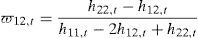

Considering a portfolio that combines the large and medium-firm indexes and assuming a mean–variance utility function, the optimal portfolio holdings of the large firm index are,

The optimal portfolio holdings for the medium-firm index would therefore be 1 − ϖ_12,t.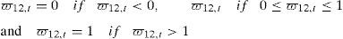

We also estimate the risk minimizing hedge ratios for these indexes by using the ratio proposed by Kroner and Sultan (1993) who show that to minimize the risk of a portfolio an investor should short $β of the second index for each $1 long in the first index. This ratio is given by:

Furthermore, each optimal portfolio holding in period t is used to calculate the expected return and volatility (measured by the standard deviation) of each portfolio in period t + 1. We follow two main objectives based on Markowitz portfolio selection procedures: (i) to determine the portfolio which holds the minimum volatility values¹⁰; and (ii) to analyze the expected return results in the event of finding the perfect combination of minimum risk and maximum return.

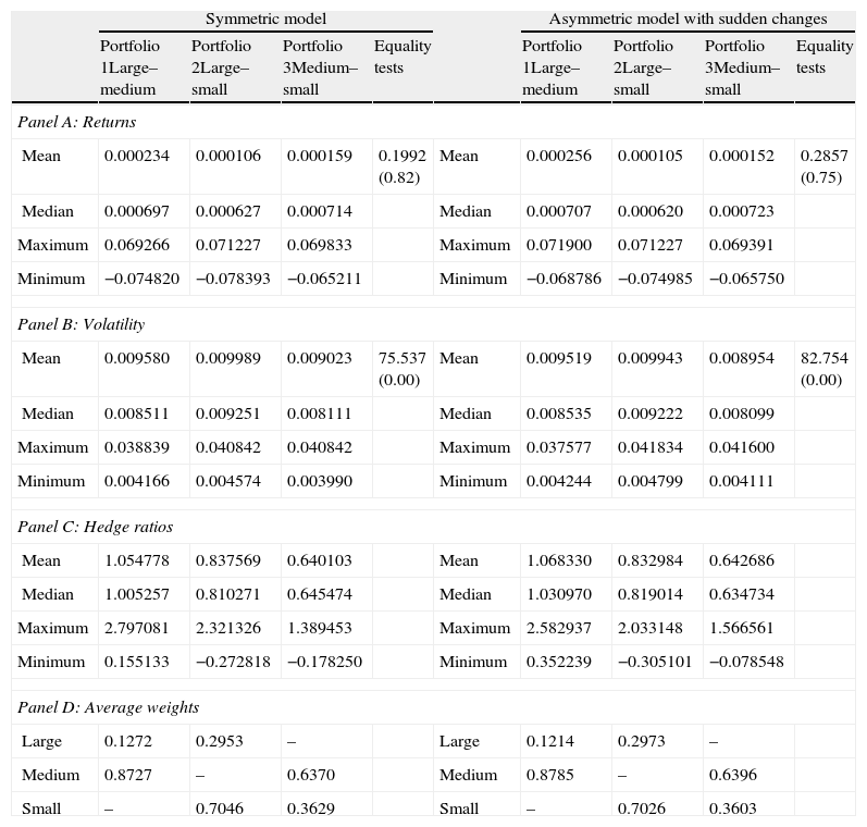
Table 5 reports results in terms of expected returns, volatility, hedge ratios and average weights for each risk minimizing portfolio constructed by the combination of pairs of indexes and employing conditional variance and covariance series from both symmetric and asymmetric multivariate GARCH models.

Table 5.

Risk minimizing portfolios.

	Symmetric model					Asymmetric model with sudden changes
	Portfolio 1Large–medium	Portfolio 2Large–small	Portfolio 3Medium–small	Equality tests		Portfolio 1Large–medium	Portfolio 2Large–small	Portfolio 3Medium–small	Equality tests
Panel A: Returns
Mean	0.000234	0.000106	0.000159	0.1992 (0.82)	Mean	0.000256	0.000105	0.000152	0.2857 (0.75)
Median	0.000697	0.000627	0.000714		Median	0.000707	0.000620	0.000723
Maximum	0.069266	0.071227	0.069833		Maximum	0.071900	0.071227	0.069391
Minimum	−0.074820	−0.078393	−0.065211		Minimum	−0.068786	−0.074985	−0.065750
Panel B: Volatility
Mean	0.009580	0.009989	0.009023	75.537 (0.00)	Mean	0.009519	0.009943	0.008954	82.754 (0.00)
Median	0.008511	0.009251	0.008111		Median	0.008535	0.009222	0.008099
Maximum	0.038839	0.040842	0.040842		Maximum	0.037577	0.041834	0.041600
Minimum	0.004166	0.004574	0.003990		Minimum	0.004244	0.004799	0.004111
Panel C: Hedge ratios
Mean	1.054778	0.837569	0.640103		Mean	1.068330	0.832984	0.642686
Median	1.005257	0.810271	0.645474		Median	1.030970	0.819014	0.634734
Maximum	2.797081	2.321326	1.389453		Maximum	2.582937	2.033148	1.566561
Minimum	0.155133	−0.272818	−0.178250		Minimum	0.352239	−0.305101	−0.078548
Panel D: Average weights
Large	0.1272	0.2953	–		Large	0.1214	0.2973	–
Medium	0.8727	–	0.6370		Medium	0.8785	–	0.6396
Small	–	0.7046	0.3629		Small	–	0.7026	0.3603

Following Kroner and Ng (1998), Ewing and Malik (2005), and Hassan and Malik (2007), we calculate the composition and hedge ratios of three risk minimizing portfolios by the combination of each pair of indexes and employing conditional variance and covariance series from both symmetric and asymmetric multivariate GARCH models. Portfolio 1 is constructed by the combination of large and medium cap indexes, Portfolio 2 is constructed by the combination of large and small cap indexes, and Portfolio 3 is constructed by the combination of medium and small cap indexes. Based on the optimal portfolio holdings in period t, we calculate the expected returns and volatility (measured as standard deviation) of each portfolio in period t + 1. Panel A, B, and C show mean, median, maximum and minimum values for expected returns, volatility and hedge ratios of each portfolio. We also present results for mean equality tests using the ANOVA statistic (p-values are reported in parentheses). Finally, Panel D presents average weights of each index in the risk minimizing portfolios.

In Panel A, we observe that the combination of the large and medium cap indexes provides the higher mean returns from both symmetric (0.000234) and asymmetric (0.000256) data. However, the low values of the Anova tests of equal means lead us to not reject the null and, therefore, to not consider the differences of average returns among the three statistically significant portfolios.

Consistent with the objective of calculating the lower risk portfolio, we observe in Panel B some interesting results. Firstly, the lower mean volatility is obtained in Portfolio 3 when medium and small cap indexes are combined (with average weights of 0.63 and 0.36, respectively) from both symmetric (0.009023) and asymmetric (0.008954) data. Secondly, differences in volatility among the portfolios are statistically significant due to the clear rejection of the null of equal means in the standard deviations derived from the Anova and Welch tests. Finally, the average standard deviations are lower when data from the asymmetric model with structural breaks is used.

Moreover, we show in Panel C the average hedge ratios for the different portfolios. The value for Portfolio 1 derived from the symmetric data is 1.054, which means that to minimize the risk an investor should short 1.054€ of the large cap index for each 1€ long in the medium cap index. The other two values for Portfolio 2 (0.8373) and Portfolio 3 (0.6401) should be interpreted in the same way. In accordance with Ewing and Malik (2005) we find that in 2 out of 3 cases (Portfolios 1 and 3) these hedge ratios are lower when compared to the model that controls for the volatility regimes. Therefore, the choice of the model affects the estimated hedge ratio and ignoring the regime shifts and asymmetries would seriously lead to wrong hedging decisions.

Additionally, as an alternative way to stress the aforementioned differences between the symmetric and asymmetric models and among the estimated minimum volatility portfolios we show Figs. 2–4.

Fig. 2.

Standard deviation differences of Portfolio 3 based on symmetric and asymmetric data.

Standard deviation differences relative to Portfolio 3 (combination of medium and small cap indexes). Positive values indicate that Portfolio 3 assume higher levels of volatility when is constructed based on the symmetric specification than employing the asymmetric one.

Fig. 3.

Standard deviation differences between Portfolio 1 and Portfolio 3.

Standard deviation differences between Portfolio 1 (large and medium cap indexes) and Portfolio 3 (medium and small cap indexes) based on asymmetric data. Positive values indicate that Portfolio 1 assume higher levels of volatility than Portfolio 3.

Fig. 4.

Standard deviation differences between Portfolio 2 and Portfolio 3.

Standard deviation differences between Portfolio 2 (large and small cap indexes) and Portfolio 3 (medium and small cap indexes) based on asymmetric data. Positive values indicate that Portfolio 2 assume higher levels of volatility than Portfolio 3.

Fig. 2 reports the differences between the estimated standard deviations of Portfolio 3 using the data from the symmetric and asymmetric models. Figs. 3 and 4 report differences between the estimated standard deviations derived from the asymmetric models of Portfolios 1 and 3 and Portfolios 2 and 3, respectively. In all cases, positive values would indicate that the volatilities in the first element of the difference is higher than in the second and, therefore, the preference of the investor for the second element (which is always Portfolio 3, the combination of the medium and small cap indexes, in its asymmetric version).

We can clearly observe that in all cases the differences are mostly positive which means that the standard deviations of Portfolio 3, which combines the Ibex Medium and Small cap indexes, are lower than the first element of each difference and, for that reason, is always the preferred one in terms of volatility.¹¹

At first glance, and consistent with the objective of determining the portfolio which holds the minimum volatility values, we would choose the portfolio where the medium and small cap indexes are combined. This is consistent with their lower volatility as reported in the descriptive statistics, and with the fact that their conditional variance is less affected by other volatility and shocks than the IBEX 35.

However, in order to obtain some more conclusive results and economic implications, we analyze the optimal portfolio responses to good and bad news (positive and negative shocks). For this reason, we consider four different scenarios in order to calculate the average risk and return of each portfolio. More precisely, the scenarios are the followings: Good news is when the previous shocks of both indexes are positive, PP, (ε_1,t−1 > 0 ; ε_2,t−1 > 0); Normal news is when one of the shocks is negative, in which case, there are two possibilities: positive–negative, PN, (ε_1,t−1 > 0 ; ε_2,t−1 < 0) and negative–positive, NP, (ε_1,t−1 < 0 ; ε_2,t−1 > 0); and, finally, Bad news is when both of the previous shocks are negative, NN, (ε_1,t−1 < 0 ; ε_2,t−1 < 0).

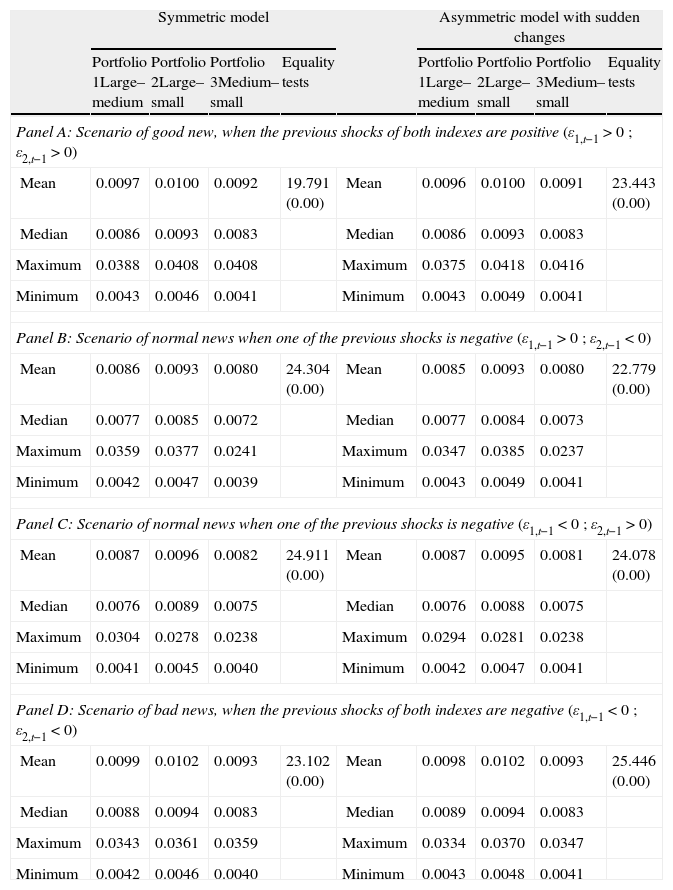
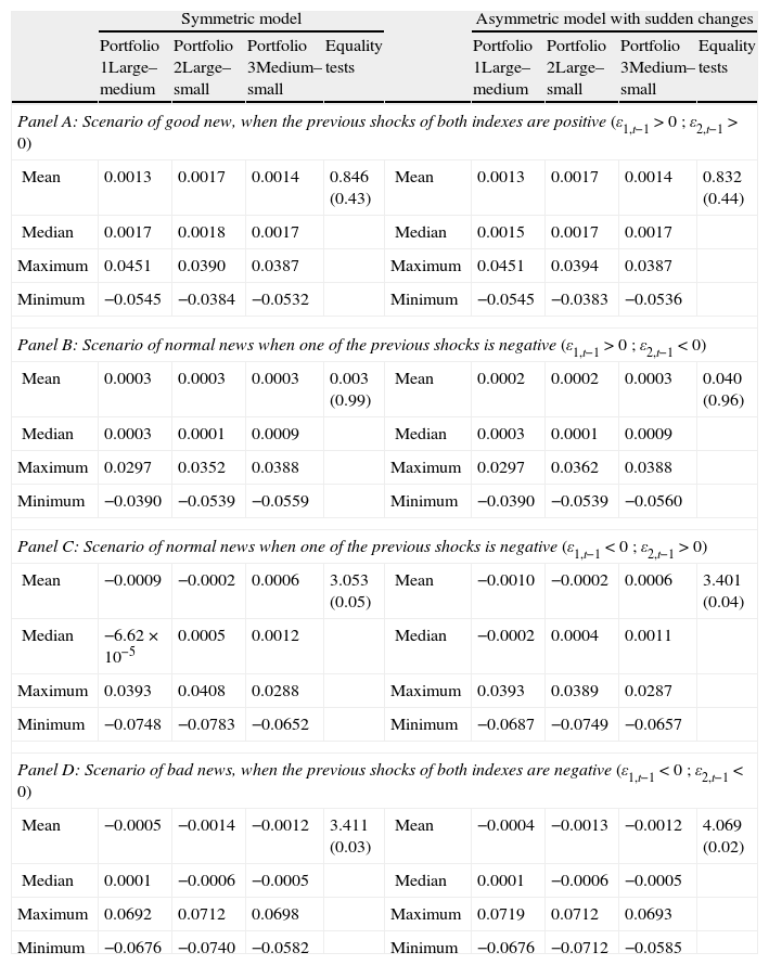
The results¹² for the estimated standard deviations and expected returns are reported in Tables 6 and 7, respectively. In all cases the lower risk values (Table 6) are achieved with Portfolio 3 which combines the Ibex Medium Cap and the Ibex Small Cap indexes. Differences among the volatilities are statistically significant due to the fact that the null of equal means is rejected in all cases. Moreover, from the results of the expected returns (Table 7) we can consider that the best combination of minimum risk and maximum return is that provided by Portfolio 3 when the negative–positive scenario is considered. This is because the minimum risk¹³ (0.0081) and maximum return (0.0006) are complemented with the rejection of the null of equal expected return means in all cases which indicates that the means returns are statistically different.

Table 6.

Risk minimizing portfolio responses to good and bad news. Volatility analysis.

	Symmetric model					Asymmetric model with sudden changes
	Portfolio 1Large–medium	Portfolio 2Large–small	Portfolio 3Medium–small	Equality tests		Portfolio 1Large–medium	Portfolio 2Large–small	Portfolio 3Medium–small	Equality tests
Panel A: Scenario of good new, when the previous shocks of both indexes are positive (ε1,t−1 > 0 ; ε2,t−1 > 0)
Mean	0.0097	0.0100	0.0092	19.791 (0.00)	Mean	0.0096	0.0100	0.0091	23.443 (0.00)
Median	0.0086	0.0093	0.0083		Median	0.0086	0.0093	0.0083
Maximum	0.0388	0.0408	0.0408		Maximum	0.0375	0.0418	0.0416
Minimum	0.0043	0.0046	0.0041		Minimum	0.0043	0.0049	0.0041
Panel B: Scenario of normal news when one of the previous shocks is negative (ε1,t−1 > 0 ; ε2,t−1 < 0)
Mean	0.0086	0.0093	0.0080	24.304 (0.00)	Mean	0.0085	0.0093	0.0080	22.779 (0.00)
Median	0.0077	0.0085	0.0072		Median	0.0077	0.0084	0.0073
Maximum	0.0359	0.0377	0.0241		Maximum	0.0347	0.0385	0.0237
Minimum	0.0042	0.0047	0.0039		Minimum	0.0043	0.0049	0.0041
Panel C: Scenario of normal news when one of the previous shocks is negative (ε1,t−1 < 0 ; ε2,t−1 > 0)
Mean	0.0087	0.0096	0.0082	24.911 (0.00)	Mean	0.0087	0.0095	0.0081	24.078 (0.00)
Median	0.0076	0.0089	0.0075		Median	0.0076	0.0088	0.0075
Maximum	0.0304	0.0278	0.0238		Maximum	0.0294	0.0281	0.0238
Minimum	0.0041	0.0045	0.0040		Minimum	0.0042	0.0047	0.0041
Panel D: Scenario of bad news, when the previous shocks of both indexes are negative (ε1,t−1 < 0 ; ε2,t−1 < 0)
Mean	0.0099	0.0102	0.0093	23.102 (0.00)	Mean	0.0098	0.0102	0.0093	25.446 (0.00)
Median	0.0088	0.0094	0.0083		Median	0.0089	0.0094	0.0083
Maximum	0.0343	0.0361	0.0359		Maximum	0.0334	0.0370	0.0347
Minimum	0.0042	0.0046	0.0040		Minimum	0.0043	0.0048	0.0041

Following Kroner and Ng (1998), Ewing and Malik (2005), and Hassan and Malik (2007), we calculate the composition of three risk minimizing portfolios by the combination of each pair of indexes and employing conditional variance and covariance series from both symmetric and asymmetric multivariate GARCH models. Portfolio 1 is constructed by the combination of large and medium cap indexes, Portfolio 2 is constructed by the combination of large and small cap indexes, and Portfolio 3 is constructed by the combination of medium and small cap indexes. Based on the optimal portfolio holdings in period t, we calculate the volatility (measured as standard deviation) of each portfolio in period t + 1 in four different scenarios: Good news is when the previous shocks of both indexes are positive; Normal news is when one of the shocks is negative, in which case, there are two possibilities: positive–negative, and negative–positive; and, Bad news is when both of the previous shocks are negative. Panel A, B, and C show mean, median, maximum and minimum volatility values of each portfolio in each scenario. We also present results for mean equality tests using the ANOVA statistic (p-values are reported in parenthesis).

Table 7.

Risk minimizing portfolio responses to good and bad news. Return analysis.

	Symmetric model					Asymmetric model with sudden changes
	Portfolio 1Large–medium	Portfolio 2Large–small	Portfolio 3Medium–small	Equality tests		Portfolio 1Large–medium	Portfolio 2Large–small	Portfolio 3Medium–small	Equality tests
Panel A: Scenario of good new, when the previous shocks of both indexes are positive (ε1,t−1 > 0 ; ε2,t−1 > 0)
Mean	0.0013	0.0017	0.0014	0.846 (0.43)	Mean	0.0013	0.0017	0.0014	0.832 (0.44)
Median	0.0017	0.0018	0.0017		Median	0.0015	0.0017	0.0017
Maximum	0.0451	0.0390	0.0387		Maximum	0.0451	0.0394	0.0387
Minimum	−0.0545	−0.0384	−0.0532		Minimum	−0.0545	−0.0383	−0.0536
Panel B: Scenario of normal news when one of the previous shocks is negative (ε1,t−1 > 0 ; ε2,t−1 < 0)
Mean	0.0003	0.0003	0.0003	0.003 (0.99)	Mean	0.0002	0.0002	0.0003	0.040 (0.96)
Median	0.0003	0.0001	0.0009		Median	0.0003	0.0001	0.0009
Maximum	0.0297	0.0352	0.0388		Maximum	0.0297	0.0362	0.0388
Minimum	−0.0390	−0.0539	−0.0559		Minimum	−0.0390	−0.0539	−0.0560
Panel C: Scenario of normal news when one of the previous shocks is negative (ε1,t−1 < 0 ; ε2,t−1 > 0)
Mean	−0.0009	−0.0002	0.0006	3.053 (0.05)	Mean	−0.0010	−0.0002	0.0006	3.401 (0.04)
Median	−6.62 × 10^−5	0.0005	0.0012		Median	−0.0002	0.0004	0.0011
Maximum	0.0393	0.0408	0.0288		Maximum	0.0393	0.0389	0.0287
Minimum	−0.0748	−0.0783	−0.0652		Minimum	−0.0687	−0.0749	−0.0657
Panel D: Scenario of bad news, when the previous shocks of both indexes are negative (ε1,t−1 < 0 ; ε2,t−1 < 0)
Mean	−0.0005	−0.0014	−0.0012	3.411 (0.03)	Mean	−0.0004	−0.0013	−0.0012	4.069 (0.02)
Median	0.0001	−0.0006	−0.0005		Median	0.0001	−0.0006	−0.0005
Maximum	0.0692	0.0712	0.0698		Maximum	0.0719	0.0712	0.0693
Minimum	−0.0676	−0.0740	−0.0582		Minimum	−0.0676	−0.0712	−0.0585

Following Kroner and Ng (1998), Ewing and Malik (2005), and Hassan and Malik (2007), we calculate the composition of three risk minimizing portfolios by the combination of each pair of indexes and employing conditional variance and covariance series from both symmetric and asymmetric multivariate GARCH models. Portfolio 1 is constructed by the combination of large and medium cap indexes, Portfolio 2 is constructed by the combination of large and small cap indexes, and Portfolio 3 is constructed by the combination of medium and small cap indexes. Based on the optimal portfolio holdings in period t, we calculate the expected return of each portfolio in period t + 1 in four different scenarios: Good news is when the previous shocks of both indexes are positive; Normal news is when one of the shocks is negative, in which case, there are two possibilities: positive–negative, and negative–positive; and, Bad news is when both of the previous shocks are negative. Panel A, B, and C show mean, median, maximum and minimum expected return values of each portfolio in each scenario. We also present results for mean equality tests using the ANOVA statistic (p-values are reported in parenthesis).

5

Conclusions

This paper initially examines the transmission of volatility and shocks among three relevant indexes (IBEX 35, IBEX MEDIUM CAP, and IBEX SMALL CAP) which were created as a reference for large, medium and small capitalization companies in the Spanish stock market. Initially, we find that all the indexes are directly and indirectly affected by the others, being especially significant the bi-directional relationship between the medium and small firms. However, these relationships disappear when asymmetries and structural breaks are taken into account.

In order to analyze the economic implications of our results, we calculate the optimal invested portfolio holdings. Considering different scenarios we demonstrate that the minimum risk portfolio is that which combines the IBEX MEDIUM CAP and the IBEX SMALL CAP indexes (with a higher weight for the medium index). This implies that investors should keep a close eye on that portfolio which also obtains the best return results in some of the analyzed situations. These results add a new point of view to the analysis of volatility because we show that the reduced volatility of medium and small firm indexes makes them an interesting investment option even in times of recession.

To sum up, we want to point out that the results of multivariate GARCH models can be used by financial market participants to make optimal portfolio allocation decisions. These results have important implications for building accurate asset pricing models, forecasting volatility and, consequently, understanding the Spanish stock market.