


The predictability of market performance is a matter of interest not only for traders and investors in financial market instruments but also for those attempting to understand the dynamics of these markets. According to the efficient market hypothesis, the price of an asset is a perfect reflection of all the information available, and consequently, it is not possible to capitalize on “undervalued or overvalued” asset; thus making market price prediction practically impossible. However, there are several groups of reasons (for example, transaction costs) that have led some economists to believe that prices are at least partially predictable. In this context, this study tries to evaluate the gradual information diffusion theory proposed by Hong et al. (2007) where industries with valuable, fundamental economic information tend lead the equity market as well as the economic activity. This hypothesis is not supported in the case of Spain, where company characteristics, and especially size, may be more relevant in understanding lead-lag patterns.
Predictability of market performance is a matter of interest not only for traders and investors in financial market instruments but also for institutions, such as securities regulators, in their attempt to understand the dynamics of these markets. The efficient market hypothesis states that market prediction is not possible because the price of an asset is the perfect reflection of all the information available, and consequently, it is not possible to capitalize on an “undervalued or overvalued” asset. However, there are several groups of reasons (for example, transaction costs or the existence of information that is not freely available) that have led some economists to believe that prices are partially predictable. In fact, during the nineties, papers related to the identification of lead-lag patterns in the equity markets abounded.
Some of these studies, based on behavioural finance, state that the information diffusion process is relevant in the predictability of stock prices. The rate of reaction to news plays an important role in the lead-lag effect. Other papers deal with “stock market overreaction” and explain lead-lag patterns in terms of the existence of an excess of optimism or pessimism. Company characteristics and other financial variables have often been presented as good explanations of lead-lag patterns. In particular, the company size plays an important role. More recently, the study of Hong et al. (2007) proposed another gradual information diffusion theory, where industries with valuable fundamental economic information tend to lead the equity market as well as the economic activity. This is the hypothesis we have tested for Spanish equity markets and other European markets.
According to our results, Spanish industries that are leaders in the stock market are not necessarily leaders in economic activity. As a consequence, the gradual information diffusion theory does not hold up for Spanish data. In general, Spanish industries in a leading market position are characterized by the presence of big companies (oil, telecom, utilities, retail), thus suggesting that company characteristics may play a significant role in the estimated lead-lag patterns. The results obtained in other European countries reveal similar conclusions, highlighting the fact that differences in characteristics of companies listed in European stock markets with respect to those listed in US markets may explain these findings.
The remainder of the paper is structured as follows: Section 2 summarizes the background and academic literature regarding the potential existence of lead-lags patterns in equity markets. Section 3 describes the data regarding equity markets (broad market index and industry indexes) and macroeconomic variables. Section 4 presents the evidence related to the presence of these lead-lag patterns in the Spanish equity market and provides potential explanations. Section 5 performs a similar analysis for other European markets. Finally, Section 6 lays out the main conclusions.
2Theoretical background and dataPredicting asset returns and, consequently, identifying lead-lag patterns in financial markets are topics that have been addressed by academics from very different perspectives. In general, daily stock-price changes are determined by the interplay of the company's internal factors (fundamentals), external factors (macroeconomic trends, financial market indicators, information, …) and expectations that may have a direct or indirect effect on the price. The most concerning and controversial question is whether a stock return (industry or market) is predictable, based on a set of variables. There are many theories that have been tested in a variety of studies on investors’ ability to predict the price of an asset. No clear consensus has yet been reached on this topic according to the results of these studies.
This section presents the most important theories and evidence on the predictability of stock market prices. Our starting point must be the efficient market hypothesis, which states that the price of an asset is the perfect reflection of all the information available. Under this hypothesis, it would not be possible to capitalize on an “undervalued or overvalued” price. The efficient market hypothesis, widely accepted some years ago thanks to the famous article of Fama (1970), is usually akin with the idea of the “random walk process”. Under this process, price series are characterized in a way in which next price changes represent random departures from previous prices.
Given that the assumptions under the efficient market hypothesis may be too strong, three degrees of efficiency have been stated (strong, semi-strong and weak efficiency). Strong efficiency is the purest form of efficiency: all information in a market, public or private, is accounted for in a stock price. Not even insider information could give an investor a leading edge. Semi-strong efficiency implies that all public information is factored into a stock's current share price. Neither fundamental nor technical analysis can be used to attain superior gains. Finally, the weak efficiency hypothesis claims that all past prices of a stock are reflected in today's stock price.
The existence of transaction costs, information that is not freely available to all investors, and discrepancies among investors were often cited as sources of inefficiencies in the markets, and some economists and econometricians started to believe that prices could be at least partially predictable. During the nineties, a significant number of studies proliferated in order to understand the black box under the potential predictability of the stock market prices.
There is a group of papers on behavioural finance in which the information diffusion process is relevant in the case of stock price predictability. According to Lo and MacKinlay (1990), Brennan et al. (1993) and Badrinath et al. (1995), the rate of reaction to information plays a prominent role in the lead-lag effect. In some studies, the possibility of some investors underreacting to information may cause serial correlation across stock prices and consequently predictability.
Another group of papers on behavioural finance are related to “stock market overreaction” (see, for example, DeBondt and Thaler, 1985; DeLong et al., 1989). Under these theories, there is a tendency for stock-market prices to “overreact” due to an excess of optimism or pessimism that may trigger prices to deviate systematically from their fundamentals values. After a period of time, these prices exhibit a reversion to the mean. In these cases, the predictability of the asset price is due mainly to the negative serial autocorrelation of stock prices.
Some studies have attempted to explain stock price predictability based on some financial parameters (dividend yield, interest rates…) and company characteristics. Company size, the level of analyst coverage or trading volumes have been the most commonly examined characteristics in these studies. Regarding size, Hou (2007) found that company size (in function of the market capitalization) may be a key factor, since big company prices tend to lead small company prices within the industry. Lo and MacKinlay (1990) also proved that company size plays an important role, since the lead-lag patterns relies on it, as big companies lead small ones. Several reasons have been argued with regards to small companies exhibiting this delay: differences in liquidity (or trading volumes), differences in analyst coverage or in institutional ownership (Badrinath et al., 1995; Menzly and Ozbas, 2010).
The relevance of differences in trading volumes (measured as the turnover of 16 portfolios) was highlighted in Chordia and Swaminathan (2000). They demonstrate that high trading volume portfolios lead low trading volume portfolios, as a consequence of the ability of the high trading volume portfolio to adjust faster to information. The role of the analyst coverage was shown by Brennan et al. (1993).
Hong et al. (2007) addressed the matter of the information diffusion theory differently. They focused on predicting the aggregate stock market return based on individual industry returns and propose a gradual information diffusion model where only industries with information about market fundamentals can lead the market. If these industries exhibit information on market fundamentals, they should also lead the economic activity. The authors, who performed this exercise for the US stock market using data from 34 industries, found a strong correlation between an industry's ability to predict the stock market and economic activity. However, Tse (2015), who re-examined these results using extended data (48 industries) and the period of time, found substantially fewer industries with the ability to predict the stock market.
In this paper, we apply the methodology of Hong et al. (2007) for the case of Spain as well as for some of the other European countries (core and peripheral countries). In general, we find some evidence of predictability of stock market returns, although industries that lead the market do not generally lead economic activity. We argue that, in future work, lead-lag patterns in Spain, and possibly in other European countries, should be explored in terms of the characteristics of the companies. Examination of causality relationships between the stock market and industries may also be interesting.
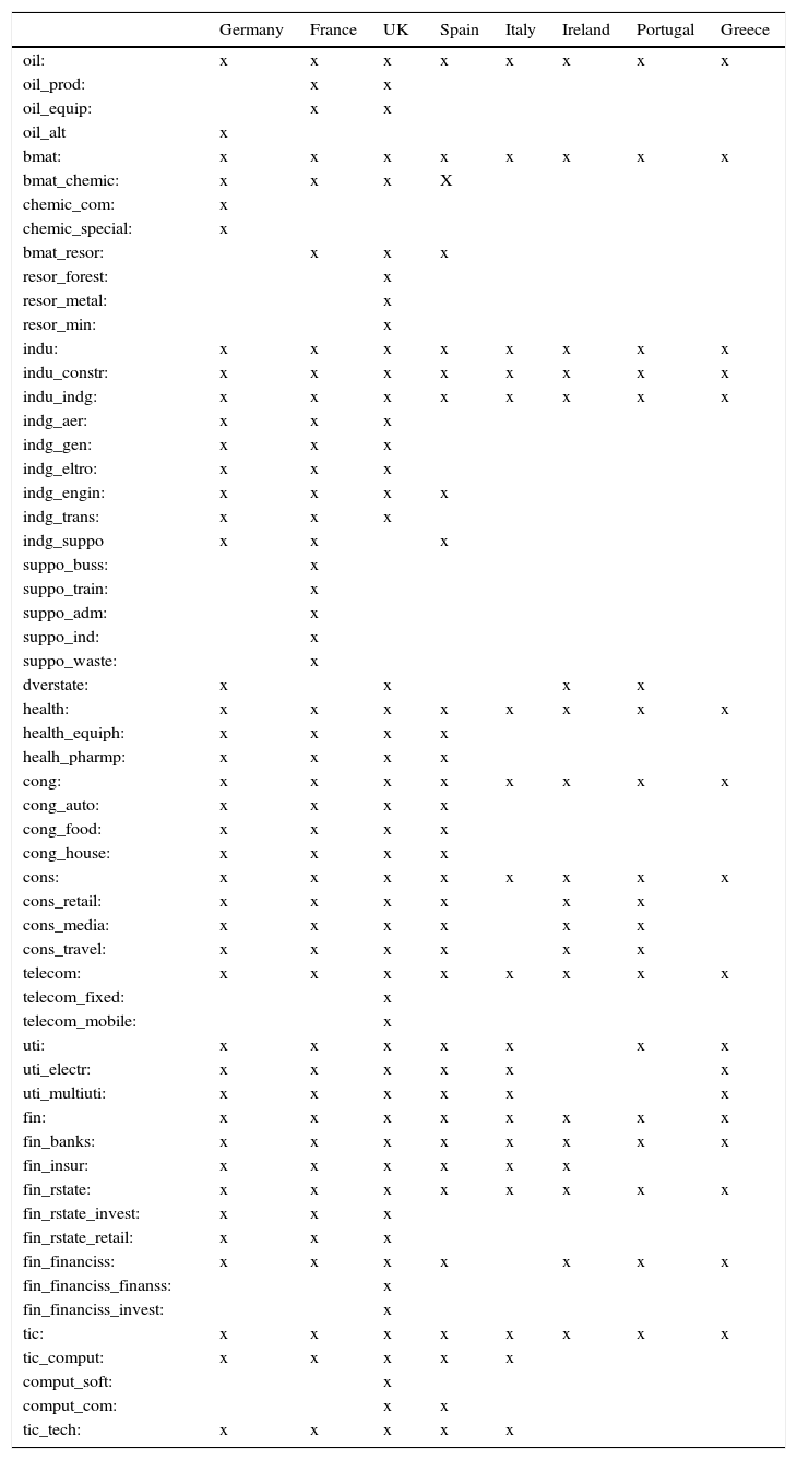
Our data comes from a single commercial database: Thomson Datastream. In the case of equity market variables, we used monthly data on the benchmark broad market equity index and industry sector indexes according to Datastream classification. This fact introduces a higher level of comparability among results from different countries, although it is important to mention that there is some heterogeneity in the availability of data at the industry level. Fig. 1 shows the industry classification provided by Thomson Datastream with the maximum degree of granularity. In general, we have data on most of the industries for the core European countries, but we have a smaller number of industries for the rest of the countries (see Table A3). We required data starting in 1999. For Spain, we have information on 24 industries (orange-shaded blocks in Fig. 1), which compares well with other European countries.
. Source: Thomson Datastream classification of equity market industries.")
Other financial variables used in our predictive regressions include: three-month interest rates (Treasury bills or interbank market), dividend yield, equity market volatility, default spread, and a stress indicator of the financial system (for Spain).1 Data on three-month interest rates were used to compute excess returns for the broad market and the industry indexes. Default spread is defined as the difference between the yield of BBB and AAA-rated bonds. Considering that bond indices with these characteristics only exist for the UK and Eurozone as a whole, we decided to adjust the Eurozone default spread with sovereign credit risk premia in order to obtain different series for this indicator in each European country. The sovereign credit risk was defined as the difference between one European country's ten-year government bond yield and Germany's ten-year government bond yield.
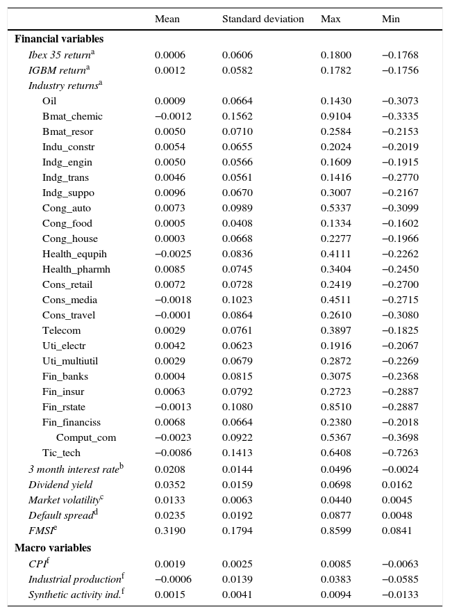
We also use the following macroeconomic variables: monthly changes in consumer prices (seasonally adjusted), monthly changes in industrial production (seasonally adjusted), and monthly changes in a synthetic indicator of economic activity. For some European countries (for example, in Spain and Italy), we have synthetic indicators provided by the Ministry of Economy. When they are not available, we used OECD leading-activity indicators. Table A1 provides some statistics on the Spanish data available.
3Evidence for SpainWe estimate two predictive regressions: regressions involving market and industry returns and regressions involving economic activity and industry returns. We want to identify industries that lead the general trend of the market and test if these industries also lead economic activity. The idea is that if industries lead the market because they have significant economic information, then they should also lead economic activity. If it is not the case, we can think of alternative explanations, for example, those that relate lead-lag patterns to some characteristics of the companies (or industries) such as size and liquidity. The first predictive regression involves excess return on the market portfolio and excess return of industry portfolios. The general equation is:
where rmt is the excess return on the market in month t, ri,t−1 is the excess return of industry portfolio i lagged one month and Xt−1 is an additional set of market predictors. We have 24 regressions with 203 observations in each of them. The main advantage of this multiple estimation is related to the possibility of measuring the effect of each industry on market return. The disadvantage is related to the omitted variables problem. We could also compute one pooled regression with all industries. In this case, the presence of high correlation across industries may be detrimental for the estimation of individual industry effects. Moreover, the low number of observations may imply high standard errors and consequently less precise estimations. In practice, the results are not very different estimating individual or pooled regressions.
We use an analysis that combines Time Series for several Cross Section (TSCS) industries. In order to estimate our predictive regressions, we use an OLS estimation (Ordinary Last Square) for our TSCS data, taking into account that the parameter estimators would be consistent but inefficient because of the potential violation of some standard assumptions regarding the error term. In particular, we must account for potential correlation of the residuals across industries as well as for serial correlation. In order to deal with these problems we have applied the Panel Corrected Standard Errors proposed by Beck and Katz (1995). We retain the OLS parameter estimators, adjusting the standard errors for cross-industry correlation in the error term.2 The standard errors are also corrected for serial correlation and heteroscedasticity. The benchmark model includes common coefficients for the predictive variables (lagged values of stock market return, inflation, dividend yield, volatility, treasury bill interest rate and default spread) and cross section specific regressors for the industry returns in t−1. We have also estimated the model allowing for changes in all coefficients, obtaining very similar results.
Our main interest is on the estimates of beta that measure the ability of each industry to predict the market. However, we will also pay attention to the results of the other macro-financial controls, in order to make a comparison with other previous studies. In this respect, Ang and Bekaert (2006) found a positive relationship between dividend yield and market performance and a negative relationship between interest rates and market performance in the US market. These results are consistent with those obtained by Hong et al. (2007) and by Rapach et al. (2013). In the latter paper, the dividend yield is found as a significant predictor of the stock market in the UK (positive relationship) while the interest rate is found to be statistically significant in Germany, UK, Canada, and Netherlands, affecting the return of the stock market negatively. Moreover, Fama and French (1989) proved that the dividend yield is able to forecast the stock market return in the US, pointing out that the higher the dividend yield the higher the return of the stock market.3 Finally, some studies conducted at short and long-term horizons have suggested a negative relationship between inflation and stock market return for longer horizons4 (more than one year).
The second predictive regression involves economic activity and industry returns. The general equation is:
where ipit is the monthly change of the economic activity indicator, ri,t−1 is the excess return of industry portfolio i lagged one month and LXt−1 is the same set of controls as in (1), except that we include some lags of the economic activity indicator. We estimate (2) in the same way we did for Eq. (1), accounting for potential cross-correlation across industries.3.1Predictive regressions involving market and industry returns
Results of predictive regressions involving market and industry returns are presented in Table 1. Current stock market return (excess of) is considered our dependent variable and past industry returns (and other controls) are considered potential predictors. We compute 24 regressions including data from January 1999 to December 2015. Upper left part of Table 1 presents results for the general controls (the coefficients are restricted to be the same) whereas the rest of the table presents individual results for each industry portfolio. Results for the alternative pooled regression are similar and will be omitted in this paper for brevity.
Predictive regression involving market and industry returns (Ibex 35).
| Dependent variable: rm (Ibex 35) | |||
|---|---|---|---|
| General controls | Industries (−1) (cont.) | ||
| Constant | −0.270*** (0.104) | CONG_AUTO | 0.024 (0.040) |
| rm (−1) | −0.028 (0.077) | CONG_FOOD | −0.125 (0.093) |
| CPI (−1) | 0.219 (1.875) | CONG_HOUSE | −0.073 (0.060) |
| Treasury Bills (3m) (−1) | −0.981* (0.514) | CONS_RETAIL | −0.115** (0.049) |
| Dividend yield (−1) | −0.040* (0.022) | CONS_MEDIA | −0.007 (0.035) |
| Market Volatility (−1) | −0.030** (0.013) | CONS_TRAVEL | −0.071* (0.040) |
| Default spread (−1) | 0.009** (0.004) | HEALTH_EQUIPH | −0.097** (0.047) |
| HEALTH_PHARM | −0.046 (0.051) | ||
| Industries (−1) | TELECOM | 0.056* (0.033) | |
| OIL | −0.051 (0.050) | UTI_ELECTR | −0.142*** (0.048) |
| BMAT_CHEMIC | −0.028 (0.024) | UTI_MULTIUTIL | −0.096** (0.050) |
| BMAT_RESOR | −0.004 (0.049) | FIN_BANKS | −0.005 (0.027) |
| INDU_CONSTR | −0.087* (0.050) | FIN_INSUR | −0.052 (0.043) |
| INDG_ENGIN | −0.022 (0.065) | FIN_RSTATE | 0.010 (0.037) |
| INDG_TRANS | −0.035 (0.064) | FIN_FINANCISS | −0.043 (0.051) |
| INDG_SUPPO | −0.030 (0.056) | TIC_COMPUT | −0.046 (0.040) |
| TIC_TECH | −0.004 (0.028) | ||
| R2 | 0.0509 | ||
The results from forecasting the market return (Ibex 35) in month t using variables at month t−1. General controls are: rm (the Ibex 35 excess value portfolio return), CPI (the inflation rate); 3 month Treasury bill interest rates; dividend yield, market volatility and default spread. The other predictors are the 24 industry returns. Least square estimates, standard errors (in parentheses) and adjusted R2 are displayed. The standard errors are adjusted for cross-industry correlation in the error terms using an estimate of the covariance matrix computed with estimated residuals from the 24 regressions. The standard errors also include serial correlation and heteroskedasticity correction. Monthly data from January 1999 to December 2015.
Regarding industries, we find 7 industries out of 24 that are able to lead the market. These industries are related to the construction sector, consumer services, telecommunications, utilities and health. The most significant coefficients are found for utility companies: electricity and multi-utility companies. Only telecom companies exhibit a positive relationship between its past return and current return of the broad market. For the rest of the industries the relationship identified between past industry returns and current broad market returns is negative. In industries considered as relevant suppliers for other industries or economic activities, such as utilities, other studies also find this negative relationship and argue that an increase in the returns of these companies is usually related to high commodity prices that erode the business of the rest of the companies. Other negative correlations may be explained in terms of the “overreaction effect” that has also been identified in previous studies.
In Hong et al. (2007), 14 out of 34 industries are found to lead the market. Some of the industries are involved with commodities or more generally with some industrial activity. Commercial real estate, retail, and financial services are also found to be significant predictors of the market. Comparing these results with those obtained for Spain, we see two common predictive industries: retail and utilities. However, the signs of the estimated coefficients diverge: they are positive for the US case and negative for Spain, suggesting that the “overreaction effect” may be much more relevant in the Spanish case. As we will see later, the negative relationship between past utility industry returns and current market returns is also found in other European countries. Finally, we should bear in mind that results of Tsay (2015) point to a less significant ability of industries to predict the market. In general, European stock markets are different from the US stock markets, as US stock markets are characterized by a high number of small and mid size industrial companies, whereas in Europe, equity markets are much more concentrated, being big banks, utilities and telecom companies very significant.
Regarding the predicting ability of our general controls and macro-financial regressors, we do not find a significant persistence in the returns of the broad market: past market returns do not (statistically) predict current market returns. This is also found in the extended model study of Hong et al. (2007). Other similarities with our reference paper are related to the identified relationship between past interest rates and current market return and between past default spread and current market return. In particular, we find that past Treasury bills interest rates are negatively related to current stock market returns and that past default spreads are positive related to current stock market returns. Evidence for volatility is mixed. We obtain a negative relationship between past volatility and current stock market returns, whereas in Hong et al. (2007) a positive relationship is found. The results in other studies do not point clearly to a specific relationship between these two magnitudes. In our case, we think that our result makes sense: past periods of high level of volatility in the market are usually followed by periods of decreases in equity prices.
The most significant difference with the study by Hong et al. (2007) and with other relevant papers is related to the relationship between past dividend yield and current market return. In general, academic papers found a positive relationship between these two variables. We obtain a negative coefficient, but it is not very significant (in statistical terms), and consequently the difference may not be very relevant. Finally, we find that inflation is not able to predict the market.
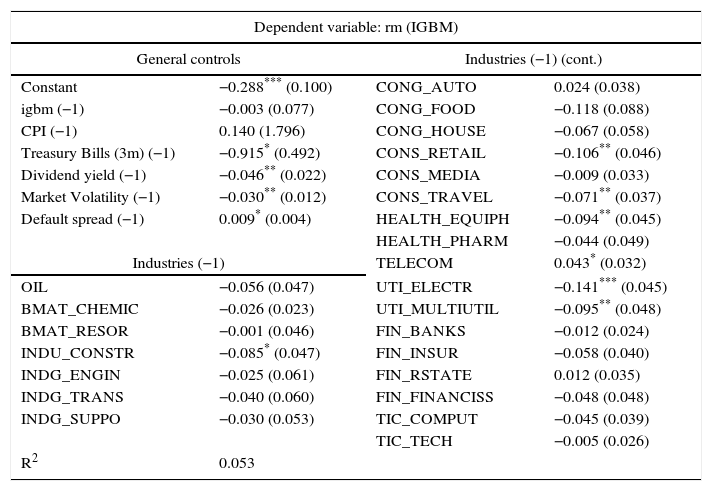
Alternatively, we have computed predictive regressions using IGBM index as our representative broad equity market index instead of Ibex 35, leading to similar results. The industries that lead the market are exactly the same, with very few differences in the estimated coefficients (see Table A4). Finally, we included another explanatory variable in the regressions, representing the level of stress in Spanish financial markets (FSMI). In this case, the predictive power of volatility decreases while other results are similar. The high correlation between the FMSI and the volatility of the market may explain this evidence, suggesting that these variables could be considered as substitutes.
3.2Predictive regressions involving economic activity and industry returnsUnder the theory we want to test, industries that lead the market do so because they contain relevant economic information. If this is the case, these industries should also lead the economic activity. In this section, we estimate the ability of industry portfolios to lead the economic activity and verify if these industries also lead the equity market. For this purpose, we estimate the second predictive regression involving economic activity and excess returns of industry portfolio, where industrial production and a synthetic indicator of activity are considered our dependent variables. Given that GDP data is only available on a quarterly basis, we chose industrial production and a synthetic indicator of activity as the best representative indicators of the economic activity, published on a monthly basis.
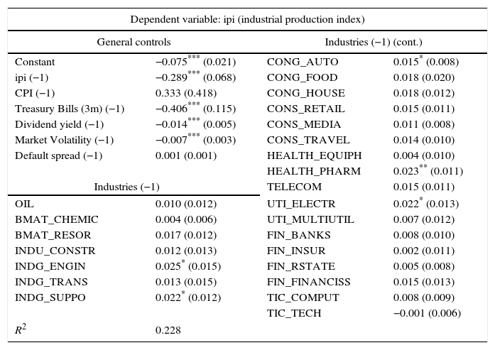
Results of the second predictive regression are presented in Table 2. Again, upper left part of the table presents the results for the macro-financial controls, whereas the rest of the table presents individual results for each industry portfolio. Regarding the predictive power of industry returns, we find that 5 out of 24 industries lead industrial production. All of them are related to industrial sectors: engine, auto, utilities, and pharmaceuticals sectors. According to the estimates, the relationship between past industry returns and current industrial production growth is always positive; in other words, increases in the equity returns of these industries are usually followed by increases in industrial production. Comparing these results with those of Table 1, we find scarce coincidence between industries that lead the equity market and industries that lead industrial production. Only health companies and utilities lead both equity market and industrial production, although the signs of the estimated coefficients are not the same.
Predictive regression involving economic activity and industry returns (ipi).
| Dependent variable: ipi (industrial production index) | |||
|---|---|---|---|
| General controls | Industries (−1) (cont.) | ||
| Constant | −0.075*** (0.021) | CONG_AUTO | 0.015* (0.008) |
| ipi (−1) | −0.289*** (0.068) | CONG_FOOD | 0.018 (0.020) |
| CPI (−1) | 0.333 (0.418) | CONG_HOUSE | 0.018 (0.012) |
| Treasury Bills (3m) (−1) | −0.406*** (0.115) | CONS_RETAIL | 0.015 (0.011) |
| Dividend yield (−1) | −0.014*** (0.005) | CONS_MEDIA | 0.011 (0.008) |
| Market Volatility (−1) | −0.007*** (0.003) | CONS_TRAVEL | 0.014 (0.010) |
| Default spread (−1) | 0.001 (0.001) | HEALTH_EQUIPH | 0.004 (0.010) |
| HEALTH_PHARM | 0.023** (0.011) | ||
| Industries (−1) | TELECOM | 0.015 (0.011) | |
| OIL | 0.010 (0.012) | UTI_ELECTR | 0.022* (0.013) |
| BMAT_CHEMIC | 0.004 (0.006) | UTI_MULTIUTIL | 0.007 (0.012) |
| BMAT_RESOR | 0.017 (0.012) | FIN_BANKS | 0.008 (0.010) |
| INDU_CONSTR | 0.012 (0.013) | FIN_INSUR | 0.002 (0.011) |
| INDG_ENGIN | 0.025* (0.015) | FIN_RSTATE | 0.005 (0.008) |
| INDG_TRANS | 0.013 (0.015) | FIN_FINANCISS | 0.015 (0.013) |
| INDG_SUPPO | 0.022* (0.012) | TIC_COMPUT | 0.008 (0.009) |
| TIC_TECH | −0.001 (0.006) | ||
| R2 | 0.228 | ||
The results from forecasting the industrial production growth (ipi) in month t using variables at month t−1. General controls are: ipi (3 lags are included, although only results for the first lag are presented), CPI (the inflation rate); 3-month Treasury bill interest rates; dividend yield, market volatility and default spread. The other predictors are the 24 industry returns. Least square estimates, standard errors (in parentheses) and adjusted R2 are displayed. The standard errors are adjusted for cross-industry correlation in the error terms, using an estimate of the covariance matrix computed with estimated residuals from the 24 regressions. The standard errors also include serial correlation and heteroskedasticity correction. Monthly data from January 1999 to November 2015.
Regarding the ability of controls to predict, we obtain significant evidence of persistence in industrial production changes in contrast with the results for the broad market equity excess return. With respect to other macroeconomic and financial indicators, we find a (statistical) negative relationship between past interest rates, past dividend yield, past equity market volatility, and current industrial production growth. Inflation and default spread are not found as relevant predictors of economic activity.
The analysis performed with US data by Hong et al. (2007) found a high level of coincidence between industries leading the market and industries leading economic activity. Moreover, the way of leading the market and the economic activity was homogeneous: industries that exhibited a positive relationship between past returns and current market returns also showed a positive relationship between past returns and current industrial production. In this case, the authors found support for the gradual information diffusion theory they were testing.
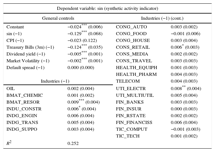
In our case, the gradual information diffusion theory does not find empirical support. However, we are going to estimate again regression 2 including the synthetic indicator of economic activity in order to verify the robustness of the previous conclusion. Table 3 presents the estimation of the predictive regressions involving economic activity and industry returns, using the synthetic indicator of economic activity as a proxy of GDP growth. This comparison is relevant because the synthetic index includes not only information of companies related to industrial activities but also to other relevant economic sectors such as services or primary sectors.
Predictive regression involving economic activity and industry returns (sin).
| Dependent variable: sin (synthetic activity indicator) | |||
|---|---|---|---|
| General controls | Industries (−1) (cont.) | ||
| Constant | −0.024*** (0.006) | CONG_AUTO | 0.003 (0.002) |
| sin (−1) | −0.129*** (0.068) | CONG_FOOD | −0.001 (0.006) |
| CPI (−1) | −0.023 (0.122) | CONG_HOUSE | 0.003 (0.004) |
| Treasury Bills (3m) (−1) | −0.124*** (0.035) | CONS_RETAIL | 0.006* (0.003) |
| Dividend yield (−1) | −0.005*** (0.001) | CONS_MEDIA | 0.002 (0.002) |
| Market Volatility (−1) | −0.002*** (0.001) | CONS_TRAVEL | 0.003 (0.003) |
| Default spread (−1) | 0.000 (0.000) | HEALTH_EQUIPH | 0.001 (0.003) |
| HEALTH_PHARM | 0.004 (0.003) | ||
| Industries (−1) | TELECOM | 0.004 (0.003) | |
| OIL | 0.002 (0.004) | UTI_ELECTR | 0.008** (0.004) |
| BMAT_CHEMIC | 0.001 (0.002) | UTI_MULTIUTIL | 0.005 (0.004) |
| BMAT_RESOR | 0.009*** (0.004) | FIN_BANKS | 0.003 (0.003) |
| INDU_CONSTR | 0.006* (0.004) | FIN_INSUR | 0.000 (0.003) |
| INDG_ENGIN | 0.006 (0.004) | FIN_RSTATE | 0.002 (0.002) |
| INDG_TRANS | 0.005 (0.004) | FIN_FINANCISS | 0.006 (0.004) |
| INDG_SUPPO | 0.003 (0.004) | TIC_COMPUT | −0.001 (0.003) |
| TIC_TECH | 0.001 (0.002) | ||
| R2 | 0.252 | ||
The results from forecasting the synthetic activity indicator growth (sin) in month t using variables at month t−1. General controls are: sin (3 lags are included, although only results for the first lag are presented), CPI (the inflation rate); 3-month Treasury bill interest rates; dividend yield, market volatility and default spread. The other predictors are the 24 industry returns. Least square estimates, standard errors (in parentheses) and adjusted R2 are displayed. The standard errors are adjusted for cross-industry correlation in the error terms, using an estimate of the covariance matrix computed with estimated residuals from the 24 regressions. The standard errors also include serial correlation and heteroskedasticity correction. Monthly data from January 1999 to September 2015.
As Table 3 depicts, we find 4 sectors out of 24 able to lead the synthetic indicator: basic material resources, industry construction, consumer services (retail) and utilities (electricity). Three of these industries (construction, consumer services and utilities) also predict the stock market return. However, and similarly to the results of the previous regression, the signs of the ability of these industries to predict the economic activity are opposite to those expected according to the gradual information diffusion theory.
As we can see, the relationship between current activity indicator growth and past performance of macro-financial variables is very similar to those shown in Table 2. The synthetic indicator of activity also shows a high degree of persistence and a negative relationship with past interest rates, past dividend yields, and past market volatility. Default spread and inflation are not found as significant predictors of economic activity.
With these results, we can say that the theoretical model of gradual information diffusion proposed by Hong et al. (2007), where industries with information about market fundamentals can lead the market and, for this reason, also lead the economic activity does not find support in the Spanish case (or at least, with the methodology and the time period used in this paper). It is possible that the differences with respect to the US study rely on the characteristics of the companies listed in the market, such as company size. Fig. 2 shows the average size of companies belonging to each industry. It is straightforward to see that industries with bigger companies (in terms of market capitalization) are the ones that lead the equity market (according to Table 1 results), with only one exception: of the banking sector.

A natural extension of this paper could be the study of lead-lag patterns in the Spanish equity markets in terms of company characteristics, and other financial parameters, and also relate these patterns with potential “overreaction” explanations. Additionally, the analysis of causality between market returns and industries return may also be relevant. As we mentioned before, there are many papers that relate stock prices predictability with, for example, the size of a company. How (2007), Lo and MacKinlay (1990) and Badrinath et al. (1995) proved that the company's size plays an important role, since the lead-lag patterns relies on it, as big companies lead small ones.
Section 4 presents a similar analysis based on data of different European countries. It is interesting to check, if the gradual information diffusion theory holds in these countries and also test potential similarities and differences between countries. Results for European core countries (Germany, France and the UK) and peripheral countries (Italy, Portugal, Ireland and Greece) are presented independently.
4Evidence for other European countriesThis section presents a similar analysis for other European countries in order to test the proposed hypothesis for some European core countries (France, Germany and UK) and peripheral countries (Italy, Greece, Ireland, and Portugal). We will explore similarities and differences with respect to Spanish and US results and will provide some explanations.
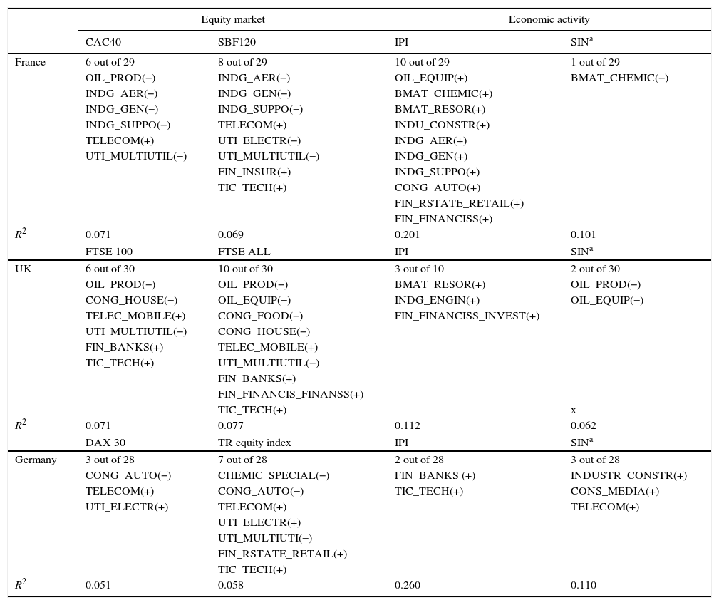
4.1Core countries (France, Germany and the UK)We estimate the same regressions as those estimated for the Spanish case, bearing in mind that European stock markets are heterogeneous and, consequently, the number of industry portfolios may be different among countries. In order to make results comparable, the estimations are carried out for the same period of time for each country, with one exception: the predictive regressions for France start in April 1999, due to the lack of data. The control variables are basically the same: the only difference is related to the interest rate data used for Germany. Instead of Treasury bills, we have used three-month interbank interest rates. Besides the industrial production indicator, we have used a composite leading indicator of economic activity for the European countries, as the synthetic indicator data is not available. In Table 4, we report the number and the name of all predictive industry portfolios with the corresponding signs of the coefficients.
Predictive regressions for European core countries: summary of results.
| Equity market | Economic activity | |||
|---|---|---|---|---|
| CAC40 | SBF120 | IPI | SINa | |
| France | 6 out of 29 | 8 out of 29 | 10 out of 29 | 1 out of 29 |
| OIL_PROD(−) | INDG_AER(−) | OIL_EQUIP(+) | BMAT_CHEMIC(−) | |
| INDG_AER(−) | INDG_GEN(−) | BMAT_CHEMIC(+) | ||
| INDG_GEN(−) | INDG_SUPPO(−) | BMAT_RESOR(+) | ||
| INDG_SUPPO(−) | TELECOM(+) | INDU_CONSTR(+) | ||
| TELECOM(+) | UTI_ELECTR(−) | INDG_AER(+) | ||
| UTI_MULTIUTIL(−) | UTI_MULTIUTIL(−) | INDG_GEN(+) | ||
| FIN_INSUR(+) | INDG_SUPPO(+) | |||
| TIC_TECH(+) | CONG_AUTO(+) | |||
| FIN_RSTATE_RETAIL(+) | ||||
| FIN_FINANCISS(+) | ||||
| R2 | 0.071 | 0.069 | 0.201 | 0.101 |
| FTSE 100 | FTSE ALL | IPI | SINa | |
| UK | 6 out of 30 | 10 out of 30 | 3 out of 10 | 2 out of 30 |
| OIL_PROD(−) | OIL_PROD(−) | BMAT_RESOR(+) | OIL_PROD(−) | |
| CONG_HOUSE(−) | OIL_EQUIP(−) | INDG_ENGIN(+) | OIL_EQUIP(−) | |
| TELEC_MOBILE(+) | CONG_FOOD(−) | FIN_FINANCISS_INVEST(+) | ||
| UTI_MULTIUTIL(−) | CONG_HOUSE(−) | |||
| FIN_BANKS(+) | TELEC_MOBILE(+) | |||
| TIC_TECH(+) | UTI_MULTIUTIL(−) | |||
| FIN_BANKS(+) | ||||
| FIN_FINANCIS_FINANSS(+) | ||||
| TIC_TECH(+) | x | |||
| R2 | 0.071 | 0.077 | 0.112 | 0.062 |
| DAX 30 | TR equity index | IPI | SINa | |
| Germany | 3 out of 28 | 7 out of 28 | 2 out of 28 | 3 out of 28 |
| CONG_AUTO(−) | CHEMIC_SPECIAL(−) | FIN_BANKS (+) | INDUSTR_CONSTR(+) | |
| TELECOM(+) | CONG_AUTO(−) | TIC_TECH(+) | CONS_MEDIA(+) | |
| UTI_ELECTR(+) | TELECOM(+) | TELECOM(+) | ||
| UTI_ELECTR(+) | ||||
| UTI_MULTIUTI(−) | ||||
| FIN_RSTATE_RETAIL(+) | ||||
| TIC_TECH(+) | ||||
| R2 | 0.051 | 0.058 | 0.260 | 0.110 |
The results of the predictive regressions for the stock market return (we use the most representative index for each country and also a general index) and one economic activity indicator (industrial production and synthetic indicator) as a function of past industry portfolios returns and other control variables (inflation, treasury bills, dividend yield, market volatility and default spread). We apply the same methodology as in the Spanish case. Thus, we retain the OLS parameter estimators, while the standard errors are computed using the estimated cross section covariance matrix, accounting for serial correlation and heteroscedasticity. Moreover, given the highest degree of autocorrelation of the synthetic indicator in all these countries, we have applied the White Transformation. For brevity, we just report the number of significant industry portfolios, listing the names of the industry portfolios able to lead stock market and economic activity, with the corresponding sign at 10% level of significance. Moreover, we report the adjusted R2. Data start in January 1999, except in France where data start in April 1999.
In the case of France, we found 6 out of 29 industry portfolios leading the CAC 40 Index. These industries are related to oil sector, industry, telecom and utilities. Three of them lead the industrial production too, but the sign of the coefficient is opposite with respect to the one observed for the stock market. As in the case of Spain, these findings do not support the gradual information diffusion hypothesis proposed by Hong et al. (2007). Moreover, industry production is leaded by 10 industry portfolios related to oil industry, basic materials, industry sector, and finance. The relationship between past industry returns and current industrial production is always positive, which is consistent with our findings for the Spanish case. In addition, when we use the SBF120 Index as our dependent variable, the number of industry portfolios leading the stock market is 8 (related to industry goods, telecom, utilities, finance sector and tic). None of the industries that lead the equity market also leads economic activity in the same direction.
In the UK, we found 6 out of 30 industry portfolios leading the FTSE100 index and 10 out of 30 leading the FTSE ALL index. The industries leading the stock market are related to oil, consumer goods, telecom, utilities, and finance. The relationship identified between past industry portfolios considered relevant suppliers for other industries (such as oil production industry and utilities) and current stock market return is negative, going hand in hand with other studies, and also with the results obtained for France. The results of predictive regressions involving past industry returns and current economic activity are mixed. When industrial production is considered as our dependent variable, we only find 3 industries with ability to predict. These industries do not lead the equity market. However, when the synthetic indicator is considered the dependent variable we found oil industries as significant predictors, being these industries also leaders of equity market returns. The gradual information diffusion hypothesis does not find significant support.
In Germany, we have found that 3 out of 28 industries leading the equity index Dax30, while 7 out of 28 lead a German equity index elaborated by Thomson Reuters (TR index). The industries leading both DAX30 and TR index are related to consumer goods, telecom and utilities. The TR index is also leaded by chemical sector, finance and technology. The results of predictive regressions involving past industry returns and current economic activity when industrial production is considered the dependent variable show only 2 out of 28 sectors able to lead the economic activity. One of them, the tic_tech sector, is also able to lead the TR equity index. When predictive regressions include the synthetic indicator as the dependent variable, three industries are found to predict the economic activity. One of them, telecom, is also able to predict the equity market returns (DAX30 ad Germ), exhibiting positive sign in both cases. Again, German data offers little support to our reference hypothesis.
In general, the findings for the European core countries are consistent with those of Spain. We observe some common industries, such as telecom and utilities, that tend to lead equity markets in all these countries and other industries able to predict the market, that are country-specific. For example, we find that industrial goods and oil sectors are significant predictors in France; finance and oil companies are relevant predictors in the UK, whereas the auto and technology corporations are important in Germany. In the case of the ability to predict economic activity, we have found much more heterogeneity among European countries. The concurrence of industries that both predict the equity market and the economic activity is scarce. This fact makes us think that industries that lead the market are not the leaders because of the economic information they show, as Hong et al. (2007) proposed, but for other reasons.
We present in Fig. 3 the average company size (market capitalisation is used as a proxy) of each equity industry in France, the UK and Germany. As in the Spanish case, most of the industries that lead the equity market are characterized by big size companies. See, for example, the telecom industry, the one with the biggest companies (on average) in all these countries and also in Spain. Oil, finance and some industrial goods industries are also big size company sectors. European equity markets are highly concentrated and characterized by big companies (telecom, banks, utilities…), that in some sense represent the underlying economic model of growth of each country, that is slightly different from the US model. For this reason, the study of lead-lag patterns taking into account company characteristics could be also appropriate for these European core countries.

Core European countries stock market: Average size of companies by industry
Source: Thomson Datastream and own calculations. Annual averages computed with data from 1999 to 2015. Full name of industries is available in Table A2.
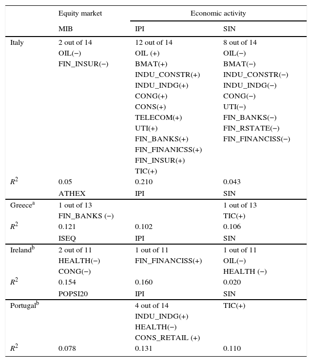
This section presents the results of our predictive regressions for other European peripheral countries: Italy, Greece, Ireland and Portugal. As in previous parts of this study we test the gradual information diffusion hypothesis proposed by Hong et al. (2007), by means of two different predictive regressions that include the excess return on market and some economic activity indicator (industrial production and the synthetic indicator) as our dependent variables. In these regressions, we try to estimate the ability of past industry returns to predict current equity market return and current economic activity. The regressions also include other general control variables, such as Treasury bills interest rates (for Greece we use the interbank interest rate, due to the lack of data), dividend yield, inflation, market volatility, and default spread. For brevity, we only report the results related to the industries found as significant predictors5 (see Table 5). In Italy and Ireland, data start in January 1999, in Portugal data start in September 1999, and in Greece, data start in September 2002. The number of industry portfolios and listed companies is significantly smaller (except in Italy) with respect to the previous cases.
Predictive regressions for European peripheral countries: summary of results.
| Equity market | Economic activity | ||
|---|---|---|---|
| MIB | IPI | SIN | |
| Italy | 2 out of 14 | 12 out of 14 | 8 out of 14 |
| OIL(−) | OIL (+) | OIL(−) | |
| FIN_INSUR(−) | BMAT(+) | BMAT(−) | |
| INDU_CONSTR(+) | INDU_CONSTR(−) | ||
| INDU_INDG(+) | INDU_INDG(−) | ||
| CONG(+) | CONG(−) | ||
| CONS(+) | UTI(−) | ||
| TELECOM(+) | FIN_BANKS(−) | ||
| UTI(+) | FIN_RSTATE(−) | ||
| FIN_BANKS(+) | FIN_FINANCISS(−) | ||
| FIN_FINANICSS(+) | |||
| FIN_INSUR(+) | |||
| TIC(+) | |||
| R2 | 0.05 | 0.210 | 0.043 |
| ATHEX | IPI | SIN | |
| Greecea | 1 out of 13 | 1 out of 13 | |
| FIN_BANKS (−) | TIC(+) | ||
| R2 | 0.121 | 0.102 | 0.106 |
| ISEQ | IPI | SIN | |
| Irelandb | 2 out of 11 | 1 out of 11 | 1 out of 11 |
| HEALTH(−) | FIN_FINANCISS(+) | OIL(−) | |
| CONG(−) | HEALTH (−) | ||
| R2 | 0.154 | 0.160 | 0.020 |
| POPSI20 | IPI | SIN | |
| Portugalb | 4 out of 14 | TIC(+) | |
| INDU_INDG(+) | |||
| HEALTH(−) | |||
| CONS_RETAIL (+) | |||
| R2 | 0.078 | 0.131 | 0.110 |
The results of the predictive regressions for the stock market return (we use the most representative index for each country and also a general index) and one economic activity indicator (industrial production and synthetic indicator) as a function of past industry portfolios returns and other control variables (inflation, treasury bills, dividend yield, market volatility and default spread). We apply the same methodology as in the Spanish case. Thus, we retain the LS parameter estimators, while the standard errors are computed using the estimated cross section covariance matrix, accounting for serial correlation and heteroscedasticity. Given the high degree of autocorrelation of the industrial production in Greece, Ireland, and Portugal and of the synthetic indicator (composite leading indicator) in all these countries, we have applied the White Transformation. For brevity, we just report the number of significant industry portfolios, listing the names of the industry portfolios able to lead stock market and economic activity, with the corresponding sign at 10% level of significance. Moreover, we report the adjusted R2. In Italy and Ireland, data start in January of 1999, in Portugal data starts in September 1999 and in Greece, data starts in September of 2002.
As we can see in Table 5, the number of industries predicting the market return is scarce. Only one or two industries are able to predict the market in each country, except in Portugal where none of the industries considered in this study has the ability to predict the market (or at least, in the way we have proceeded here, with monthly data and this sample period). Only in Italy, we find similar results to the previous European countries. In this country, we find 2 out of 14 industry portfolios with ability to lead the MIB Index.6 The predictive industry portfolios are related to oil sector and insurance sector and the sign of the coefficient is negative. The negative relationship between past oil sector returns and current market return is similar to the results of other studies and with our findings for the Spanish case and for other core countries. This kind of relationship is usually explained in terms of the potential overreaction of the market. Predictive regressions using the industrial production and the synthetic indicator as dependent variables identify more industries with predicting ability. However, as in previous cases, industries that both lead the equity market and the economic activity exhibit different sign coefficients, except in the case of the oil industry when we consider the synthetic activity indicator.
In Greece, we only find banks as a significant predictor of the equity market, but this industry does not predict the economic activity. In Ireland, 2 out of 11 industries, health and consumer goods, are able to predict the market, being the health industry also able to predict the synthetic indicator of activity. In Portugal, several industries are able to predict the industrial production but none of them predicts the equity market.
The results of these countries show very little support to the gradual information diffusion hypothesis of Hong et al. (2007). Moreover, the ability of industries to predict (equity market or activity) is very limited. Only in Italy, we find lead-lag patterns that, as in other European countries, could be studied in terms of company characteristics (see Fig. 4). In the rest of the peripheral countries analyzed in this paper, the few industries able to predict the equity market are not the ones that exhibit high size (on average). Other explanations related to these markets (for example, depth, trading volumes etc.…) could be explored. Lack of data and a short sample period may also have an impact on these results, as Tse (2015) proved for the US case.
5Conclusions
Predicting returns in equity markets has been examined in many past academic studies. Theoretically and according to the efficient market hypothesis, the price of an asset is a perfect reflection of all the information available and consequently it is not possible to capitalize on an “undervalued or overvalued” asset. In other words, price prediction would be practically impossible. However, many studies have identified several lead-lag patterns in equity markets, demonstrating that prices may in fact be partially predictable. Different reasons have been argued to explain these patterns. Some economists and econometricians argue that company characteristics and other financial indicators back these findings. In particular, company size is considered to play a significant role since big companies tend to lead small companies. The delay in small companies is related to differences in liquidity (or trading volumes), differences in analyst coverage or in institutional ownership.
Other studies focus on how valuable information spreads over the market, underscoring, for example, the rate of reaction to information. More recently, Hong et al. (2007) addressed the matter of information diffusion differently. They focused on predicting the aggregate stock market return based on individual industry returns and proposed a model of gradual information diffusion, in which only industries with information about market fundamentals can lead the market. Moreover, if these industries exhibit information on market fundamentals, they should also lead the economic activity. Hong et al. found support for this hypothesis, although Tse (2105) did not with updated data and a longer period of time.
In this paper, we tested the hypothesis proposed by Hong et al. (2007) for the Spanish market as well as for other European stock markets. Our results are similar to those of Tse (2015) but differ from the results of Hong et al. (2007). We have not found any support for their gradual information diffusion assumption in Spain or any other European country. In general, industries that lead the market are not the ones that lead economic activity. In Spain, industries that lead the market are telecom, utilities, construction, retail, and health equipment and industries that lead economic activity (industrial production) are related to utilities, some industrial goods (engineering and support), consumer goods, and health. Results for other economic activity indicators also demonstrate that the commodities and retail sectors are significant predictors. Only health companies and utilities lead both equity market and industrial production, although the signs of the estimated coefficients are not the same.
The findings of some European core countries are in line with those of Spain. We observe some common industries, such as telecom and utilities, that tend to lead equity markets in all these countries and other industries are able to predict the market that are country-specific. For example, we find that industrial goods and oil sectors are significant predictors in France; finance and oil companies are relevant predictors in the UK, whereas the auto and technology corporations are important in Germany. In the case of the ability to predict economic activity, we have found much more heterogeneity among European countries and, in general, the coincidence of industries that predict both the equity market and economic activity is scarce. In the case of other European peripheral countries, the evidence is much weaker, with the exception of Italy, where results are similar to those in Spain and other core countries. In these cases, the low number of industries and listed companies and other characteristics of the market may have played a role in the results.
In general, our conclusion points out that industries that predict the equity market in Spain and in most of the other European countries are not leaders, because they have valuable economic fundamental information. Companies in these industries are big-sized companies, suggesting that company characteristics may be relevant in the analysis of lead-lag patterns as in other academic papers. In general, European equity markets are much more concentrated than US stock markets, and this difference may be a reasonable explanation for the different results. A potential extension of this work could be the analysis of lead-lag patterns in European equity markets, considering company characteristics and testing whether differences in size, liquidity or trading volumes are important. Causality analysis may also be relevant.
See Tables A1–A4.
Summary of statistics.
| Mean | Standard deviation | Max | Min | |
|---|---|---|---|---|
| Financial variables | ||||
| Ibex 35 returna | 0.0006 | 0.0606 | 0.1800 | −0.1768 |
| IGBM returna | 0.0012 | 0.0582 | 0.1782 | −0.1756 |
| Industry returnsa | ||||
| Oil | 0.0009 | 0.0664 | 0.1430 | −0.3073 |
| Bmat_chemic | −0.0012 | 0.1562 | 0.9104 | −0.3335 |
| Bmat_resor | 0.0050 | 0.0710 | 0.2584 | −0.2153 |
| Indu_constr | 0.0054 | 0.0655 | 0.2024 | −0.2019 |
| Indg_engin | 0.0050 | 0.0566 | 0.1609 | −0.1915 |
| Indg_trans | 0.0046 | 0.0561 | 0.1416 | −0.2770 |
| Indg_suppo | 0.0096 | 0.0670 | 0.3007 | −0.2167 |
| Cong_auto | 0.0073 | 0.0989 | 0.5337 | −0.3099 |
| Cong_food | 0.0005 | 0.0408 | 0.1334 | −0.1602 |
| Cong_house | 0.0003 | 0.0668 | 0.2277 | −0.1966 |
| Health_equpih | −0.0025 | 0.0836 | 0.4111 | −0.2262 |
| Health_pharmh | 0.0085 | 0.0745 | 0.3404 | −0.2450 |
| Cons_retail | 0.0072 | 0.0728 | 0.2419 | −0.2700 |
| Cons_media | −0.0018 | 0.1023 | 0.4511 | −0.2715 |
| Cons_travel | −0.0001 | 0.0864 | 0.2610 | −0.3080 |
| Telecom | 0.0029 | 0.0761 | 0.3897 | −0.1825 |
| Uti_electr | 0.0042 | 0.0623 | 0.1916 | −0.2067 |
| Uti_multiutil | 0.0029 | 0.0679 | 0.2872 | −0.2269 |
| Fin_banks | 0.0004 | 0.0815 | 0.3075 | −0.2368 |
| Fin_insur | 0.0063 | 0.0792 | 0.2723 | −0.2887 |
| Fin_rstate | −0.0013 | 0.1080 | 0.8510 | −0.2887 |
| Fin_financiss | 0.0068 | 0.0664 | 0.2380 | −0.2018 |
| Comput_com | −0.0023 | 0.0922 | 0.5367 | −0.3698 |
| Tic_tech | −0.0086 | 0.1413 | 0.6408 | −0.7263 |
| 3 month interest rateb | 0.0208 | 0.0144 | 0.0496 | −0.0024 |
| Dividend yield | 0.0352 | 0.0159 | 0.0698 | 0.0162 |
| Market volatilityc | 0.0133 | 0.0063 | 0.0440 | 0.0045 |
| Default spreadd | 0.0235 | 0.0192 | 0.0877 | 0.0048 |
| FMSIe | 0.3190 | 0.1794 | 0.8599 | 0.0841 |
| Macro variables | ||||
| CPIf | 0.0019 | 0.0025 | 0.0085 | −0.0063 |
| Industrial productionf | −0.0006 | 0.0139 | 0.0383 | −0.0585 |
| Synthetic activity ind.f | 0.0015 | 0.0041 | 0.0094 | −0.0133 |
Number of observations: 204.
Industry classification (Thomson Datastream).
| Short name | Long name |
|---|---|
| oil: | Oil and gas |
| oil_prod: | Oil and gas producers |
| oil_equip: | Oil equipment, services and distribution |
| oil_alt: | Oil alternative |
| bmat: | Basic materials |
| bmat_chemic: | Basic materials: chemicals |
| chemic_com: | Basic materials: commodity chemicals |
| chemic_special: | Basic materials: specialized chemicals |
| bmat_resor: | Basic resources |
| resor_forest: | Basic resources: Forestry and paper |
| resor_metal: | Basic resources: Industries metals and mines |
| resor_min: | Basic resources: Mining |
| indu: | Industrials |
| indu_constr: | Industrials: Construction and Materials |
| indu_indg: | Industrials: Industrial Goods and Services |
| indg_aer: | Industrials: Industrial Goods and Services: Aerospace and defence |
| indg_gen: | Industrials: Industrial Goods and Services: General Industrials |
| indg_eltro: | Industrials: Industrial Goods and Services: Electronic and Electrical Equipment |
| indg_engin: | Industrials: Industrial Goods and Services: Industrial Engineering |
| indg_trans: | Industrials: Industrial Goods and Services: Industrial Transportation |
| indg_suppo | Industrials: Industrial Goods and Services: Support Services |
| suppo_buss: | Industrials: Industrial Goods and Services: Support Services: Business Support Services |
| suppo_train: | Industrials: Industrial Goods and Services: Support Services: Business Training and Employment Agency |
| suppo_adm: | Industrials: Industrial Goods and Services: Support Services: Financial Administration |
| suppo_ind: | Industrials: Industrial Goods and Services: Support Services: Industrial Suppliers |
| suppo_waste: | Industrials: Industrial Goods and Services: Support Services: Waste and disposal services |
| dverstate: | Diversified Real Estate Trusts |
| health: | Health care |
| health_equiph: | Health care: equipment and services |
| healh_pharmp: | Health care: pharmaceuticals and biotechnology |
| cong: | Consumer Goods |
| cong_auto: | Consumer Goods: auto and parts |
| cong_food: | Consumer Goods: food and beverages |
| cong_house: | Consumer Goods: personal and household goods |
| cons: | Consumer Services |
| cons_retail: | Consumer Services: retail |
| cons_media: | Consumer Services: media |
| cons_travel: | Consumer Services: travel and leisure |
| telecom: | Telecommunications |
| telecom_fixed: | Telecommunications: fixed line telecommunications |
| telecom_mobile: | Telecommunications: mobile telecommunications |
| uti: | Utilities |
| uti_electr: | Utilities: electricity |
| uti_multiuti: | Utilities gas, water and multi-utilities |
| fin: | Financials |
| fin_banks: | Financials: banks |
| fin_insur: | Financials: insurance |
| fin_rstate: | Financials: real estate |
| fin_rstate_invest: | Financials: real estate investment, services |
| fin_rstate_retail: | Financials: real estate investment trusts |
| fin_financiss: | Financials: financial services |
| fin_financiss_finanss: | Financials: financial services: financial services |
| fin_financiss_invest: | Financials: financial services: investment trust |
| tic: | Technology |
| tic_comput: | Technology: software and computer services |
| comput_soft: | Technology: software and computer services: software |
| comput_com: | Technology: software and computer services: computer services |
| tic_tech: | Technology: hardware and equipment |
Industry classification: available data per country.
| Germany | France | UK | Spain | Italy | Ireland | Portugal | Greece | |
|---|---|---|---|---|---|---|---|---|
| oil: | x | x | x | x | x | x | x | x |
| oil_prod: | x | x | ||||||
| oil_equip: | x | x | ||||||
| oil_alt | x | |||||||
| bmat: | x | x | x | x | x | x | x | x |
| bmat_chemic: | x | x | x | X | ||||
| chemic_com: | x | |||||||
| chemic_special: | x | |||||||
| bmat_resor: | x | x | x | |||||
| resor_forest: | x | |||||||
| resor_metal: | x | |||||||
| resor_min: | x | |||||||
| indu: | x | x | x | x | x | x | x | x |
| indu_constr: | x | x | x | x | x | x | x | x |
| indu_indg: | x | x | x | x | x | x | x | x |
| indg_aer: | x | x | x | |||||
| indg_gen: | x | x | x | |||||
| indg_eltro: | x | x | x | |||||
| indg_engin: | x | x | x | x | ||||
| indg_trans: | x | x | x | |||||
| indg_suppo | x | x | x | |||||
| suppo_buss: | x | |||||||
| suppo_train: | x | |||||||
| suppo_adm: | x | |||||||
| suppo_ind: | x | |||||||
| suppo_waste: | x | |||||||
| dverstate: | x | x | x | x | ||||
| health: | x | x | x | x | x | x | x | x |
| health_equiph: | x | x | x | x | ||||
| healh_pharmp: | x | x | x | x | ||||
| cong: | x | x | x | x | x | x | x | x |
| cong_auto: | x | x | x | x | ||||
| cong_food: | x | x | x | x | ||||
| cong_house: | x | x | x | x | ||||
| cons: | x | x | x | x | x | x | x | x |
| cons_retail: | x | x | x | x | x | x | ||
| cons_media: | x | x | x | x | x | x | ||
| cons_travel: | x | x | x | x | x | x | ||
| telecom: | x | x | x | x | x | x | x | x |
| telecom_fixed: | x | |||||||
| telecom_mobile: | x | |||||||
| uti: | x | x | x | x | x | x | x | |
| uti_electr: | x | x | x | x | x | x | ||
| uti_multiuti: | x | x | x | x | x | x | ||
| fin: | x | x | x | x | x | x | x | x |
| fin_banks: | x | x | x | x | x | x | x | x |
| fin_insur: | x | x | x | x | x | x | ||
| fin_rstate: | x | x | x | x | x | x | x | x |
| fin_rstate_invest: | x | x | x | |||||
| fin_rstate_retail: | x | x | x | |||||
| fin_financiss: | x | x | x | x | x | x | x | |
| fin_financiss_finanss: | x | |||||||
| fin_financiss_invest: | x | |||||||
| tic: | x | x | x | x | x | x | x | x |
| tic_comput: | x | x | x | x | x | |||
| comput_soft: | x | |||||||
| comput_com: | x | x | ||||||
| tic_tech: | x | x | x | x | x |
Source: Thomson Datastream and CNMV. x denotes available data for the reference period (in general, starting in 1999).
Predictive regression involving market and industry returns (IGBM).
| Dependent variable: rm (IGBM) | |||
|---|---|---|---|
| General controls | Industries (−1) (cont.) | ||
| Constant | −0.288*** (0.100) | CONG_AUTO | 0.024 (0.038) |
| igbm (−1) | −0.003 (0.077) | CONG_FOOD | −0.118 (0.088) |
| CPI (−1) | 0.140 (1.796) | CONG_HOUSE | −0.067 (0.058) |
| Treasury Bills (3m) (−1) | −0.915* (0.492) | CONS_RETAIL | −0.106** (0.046) |
| Dividend yield (−1) | −0.046** (0.022) | CONS_MEDIA | −0.009 (0.033) |
| Market Volatility (−1) | −0.030** (0.012) | CONS_TRAVEL | −0.071** (0.037) |
| Default spread (−1) | 0.009* (0.004) | HEALTH_EQUIPH | −0.094** (0.045) |
| HEALTH_PHARM | −0.044 (0.049) | ||
| Industries (−1) | TELECOM | 0.043* (0.032) | |
| OIL | −0.056 (0.047) | UTI_ELECTR | −0.141*** (0.045) |
| BMAT_CHEMIC | −0.026 (0.023) | UTI_MULTIUTIL | −0.095** (0.048) |
| BMAT_RESOR | −0.001 (0.046) | FIN_BANKS | −0.012 (0.024) |
| INDU_CONSTR | −0.085* (0.047) | FIN_INSUR | −0.058 (0.040) |
| INDG_ENGIN | −0.025 (0.061) | FIN_RSTATE | 0.012 (0.035) |
| INDG_TRANS | −0.040 (0.060) | FIN_FINANCISS | −0.048 (0.048) |
| INDG_SUPPO | −0.030 (0.053) | TIC_COMPUT | −0.045 (0.039) |
| TIC_TECH | −0.005 (0.026) | ||
| R2 | 0.053 | ||
The results from forecasting the market return (IGBM) in month t using variables at month t−1. General controls are: rm (the IGBM excess value portfolio return), CPI (the inflation rate); 3 month Treasury bill interest rates; dividend yield, market volatility and default spread. The other predictors are the 24 industry returns. Least square estimates, standard errors (in parentheses) and R2 are displayed. The standard errors are adjusted for cross-industry correlation in the error terms using an estimate of the covariance matrix computed with estimated residuals from the 24 regressions. The standard errors also include serial correlation and heteroskedasticity correction. Monthly data from January 1999 to December 2015.
See Cambón and Cerqueira (2016).
We compute an alternative covariance matrix of beta using an estimation of the covariance matrix computed with the estimated residuals from the 24 regressions.
Evidence that dividend yield is related to stock market return is also found in Rozeff (1984), Shiller (1984), Flood et al. (1986), Campbell and Shiller (1988), and Fama and French (1988b). Other interesting studies like Fama and Schwert (1977), Gultekin (1983) and, more recently, Barnes et al. (1999) showed a negative relationship between interest rates and stock market return. Fama and French (1989) also found a positive relationship between default spread and market return.
Complete results are available upon request.
Similar regressions including a higher number of industry portfolios (more desagregation of industrial sectors) point out to similar results. Sample period seems to be relevant for the estimation. Regressions starting in 2001 find also the utility industry as a significant predictor of the market.

