


This paper provides empirical evidence of how a firm's growth opportunities shape the diversification–value relationship on a sample of U.S. companies between 1998 and 2010. Our findings suggest that the negative relationship between diversification and a firm's value may reverse at high levels of diversification, and that such a U-form diversification–value relation is partly mediated by a firm's growth opportunities. Results are robust to various model specifications and after controlling for endogenous self-selection of the diversification decision.
Corporate diversification and its effect on a firm's value is a long-standing controversy in the literature. The bulk of the research is not optimistic about the implications of this strategy for value creation while, at the same time, diversified firms maintain their relevance in modern economies. Evidence in prior literature ranges from the diversification discount (the major position, as documented by Lang and Stulz, 1994; Berger and Ofek, 1995; Servaes, 1996; Stowe and Xing, 2006; Hoechle et al., 2012) to the diversification premium (Campa and Kedia, 2002; Villalonga, 2004a), and also includes the lack of any significant relationship (Villalonga, 2004b; Elsas et al., 2010). The so-called diversification puzzle remains unresolved, in both the academic and business sphere.1
The origin of this conflicting evidence also remains unclear. One prominent strand of research suggests that endogeneity may obscure the true relationship between diversification and corporate value. In this regard, Campa and Kedia (2002), Miller (2004), and Villalonga (2004b), among others, argue that certain factors affecting a firm's decision to diversify may also drive value outcomes. Overlooking such endogeneity may misattribute valuation effects to this strategy rather than to a firm's circumstances prior to the diversification decision. Once this endogeneity is controlled, Campa and Kedia (2002) report a premium. Nevertheless, Hoechle et al. (2012) cast doubt on this argument since they still obtain a discount even when endogeneity is accounted for.
Much of the empirical literature addresses the ‘average effect’ of diversification in terms of discount/premium, yet insufficient attention is paid to the cross-sectional variation of diversification value outcomes (Stein, 2003). In this sense, recent research embraces a contingent approach and posits that the impact of diversification on a firm's value may differ across firms. This relationship may be influenced by certain factors such as the institutional framework (Lins and Servaes, 1999), the industry (Santaló and Becerra, 2008), or diversity of growth opportunities (Rajan et al., 2000), to name but a few.
Among those factors, the literature has compiled suggestive yet inconclusive evidence concerning firms’ growth opportunities. Certain papers such as Bernardo and Chowdhry (2002) explain the diversification discount on the grounds that single-segment firms have more growth opportunities whereas multisegment firms may have exhausted part of these. Further supporting evidence, such as Ferris et al. (2002), reveals for a sample of international joint ventures, that diversification is value-destroying in firms with a weak cash flow position and low growth opportunities available. In contrast, other evidence (Stowe and Xing, 2006) shows that the discount remains after controlling for growth opportunities.
Based on this strand of literature, we empirically analyze whether the effect of diversification on a firm's value (discount/premium) may be contingent on growth opportunities. Firstly, we explore how diversification shapes the value of a firm's growth opportunities (more specifically, the proportion of growth opportunities value over a firm's total value, hereinafter, the growth opportunities ratio, or GOR). According to Myers (1977), growth opportunities are one component of a firm's market value (the other being the value of assets in place). Were diversification to have a significant effect on GOR, we would test whether a proportion of the total effect of diversification strategy on a firm's value is channeled via the value of growth opportunities. To address this potential mediating role of growth opportunities, we follow Baron and Kenny's (1986: 1176) causal step method. This approach is based on analyzing whether the direct effect between diversification and firm value (widely documented in prior literature) becomes weaker once the mediator GOR is accounted for in the model. If so, it will confirm that part of the impact of diversification is channeled through GOR.
Our empirical analysis is carried out on a dataset of U.S. firms from 1998 to 2010 (16,859 firm-year observations). Our empirical evidence is based on U.S. on a post-1997 sample, after coming into force the new SFAS no. 131 accounting standard. We account for the endogenous self-selection of the diversification decision using the Heckman two-step estimation. Given that this strategy is not random but is rather selected by companies, the Heckman procedure enables a firm's ex-ante underlying characteristics to be disentangled from ex-post diversification value outcomes.
Our study contributes to the existing literature by offering a deeper empirical insight into the trinomium corporate diversification, growth opportunities, and firm value, on which prior research has reached inconclusive results. Our findings show that the diversification–value relationship may take a U-form, this curvilinear effect being partly mediated by growth opportunities. Results are robust to alternative proxies and methodologies. Overall, our study provides an additional explanation to performance divergences across diversifiers.
The remainder of the paper is organized as follows. The following section describes the sample, variables, and models to be estimated. Section 3 presents our main empirical findings. The final section discusses results and conclusions.
2Sample, variables, and estimation strategy2.1Data and sample selectionThe initial sample consists of an unbalanced panel sample of U.S. public companies over the period 1998–2010. Data is extracted from Worldscope (annual data, both at the industry segment and company level2), Datastream (market data) and the U.S. Bureau of Economic Analysis3 (macroeconomic data). To build a dataset consistent with prior literature, we select the sample following the Berger and Ofek (1995) criteria.4 These criteria reduce the sample size to 28,206 firm-year observations for the period 1998–2010 (67% corresponding to pure-play firms and 33% to diversifiers).5 Next, we exclude firm-year observations with negative common equity and outlier observations of the study variables.6 Our final study sample comprises a maximum of 16,859 firm-year observations corresponding to 3190 firms.
2.2Empirical models and variablesAs a starting point, we analyze the relationship between diversification and growth opportunities by estimating Eq. (1):
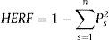
where i identifies each firm, t indicates the year of observation (from 1 to 13), α and βp are the coefficients to be estimated, and νit is the random disturbance. The dependent variable (growth opportunities ratio (GOR)) is proxied by either the market to book assets ratio (Adam and Goyal, 2008), Tobin's Q (Cao et al., 2008), or the ratio of R&D expenses to total sales (Mehran, 1995). The degree of diversification (DIVER) is computed by alternative measures to test the robustness of our empirical findings: the number of businesses at the 4-digit SIC code level (numsegments), the Herfindahl index (HERF) (Hirschman, 1964), and the entropy measure (TotalEntropy) (Jacquemin and Berry, 1979). HERF is calculated as:where ‘n’ is the number of a firm's segments (at the 4-digit SIC code level), and ‘Ps’ the proportion of the firm's sales from segment ‘s’. This index positively relates to the level of diversification, its values ranging between 0 (focused firms) and 1.
TotalEntropy is computed as follows:
where ‘Ps’ is the proportion of a firm's sales in segment ‘s’ for a company with ‘n’ different 4-digit SIC segments. The higher the total entropy, the greater the diversification, although this index has no upper boundary.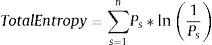
Following prior literature, we control for firm size (Andrés et al., 2005), leverage (Myers, 1977), industry effect, and time effect. Size (LTA) is estimated by the natural logarithm of the book value of total assets. Leverage (DTA) is calculated by the total ratio debt over total assets. We include dummy variables to control for the major groups of industries7 and dummies to control for the year effect.
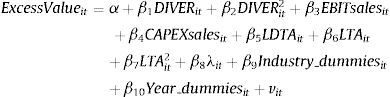
Once we have confirmed the relation between GOR and diversification, we apply Baron and Kenny's (1986) approach to test the mediation role of growth opportunities in the relation between diversification (independent variable) and excess value (dependent variable). According to Baron and Kenny (1986), GOR will act as a mediator if it meets three conditions: (i) variations in the independent variable (the ‘diversification level’) significantly account for variations in the presumed mediator (GOR); (ii) variations in the mediator (GOR) significantly account for variations in the dependent variable (excess value); and finally (iii) when the mediator (GOR) is considered, a previously significant relation between the independent and dependent variables no longer significant proves (full mediation) or becomes weaker (partial mediation).
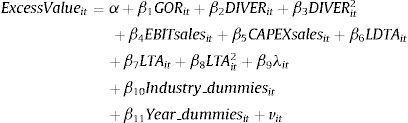
Condition (i) is tested by estimating the results of previous equation (1), while conditions (ii) and (iii) are checked by means of estimating Eqs. (2)–(4). Eqs. (2) and (3) relate excess value and diversification. Eq. (2) allows us to replicate prior research, while Eq. (3) adds a squared term for the variable of diversification:
where i identifies each firm, t indicates the year of observation (from 1 to 13), α and βp are the coefficients to be estimated, and νit is the random disturbance. The dependent variable is excess value (ExcessValue), as developed by Berger and Ofek (1995), and is defined as the natural log of a firm's market value to its imputed value.8 This measure assesses the diversification discount/premium by comparing the diversified firm's value against the value of an equivalent portfolio of unisegment firms. Moreover, in line with prior literature (Berger and Ofek, 1995; Campa and Kedia, 2002; Santaló and Becerra, 2008), we control for profitability, level of current investment, financial leverage, firm size (and its square), industry (Industry_dummies), and year effect (Year_dummies). Profitability is estimated by the EBIT to sales ratio (EBITsales), and the level of investment by capital expenditures to total sales ratio (CAPEXsales). Financial leverage is measured by the ratio of long-term debt to total assets (LDTA), and firm size is approximated by the natural logarithm of the book value of total assets (LTA).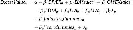
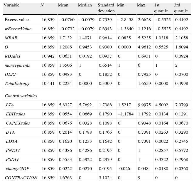
A summary of the descriptive statistics of our study's variables is shown in Table 1. Overall, the number of a firm's segments ranges between 1 and 6 in the sample. We also observe an average discount (−0.0760).
Summary statistics of variables for the full sample (1998–2010).
| Variable | N | Mean | Median | Standard deviation | Min. | Max. | 1st quartile | 3rd quartile |
| Excess value | 16,859 | −0.0760 | −0.0079 | 0.7939 | −2.8458 | 2.6628 | −0.5525 | 0.4192 |
| wExcessValue | 16,859 | −0.0732 | −0.0079 | 0.6943 | −1.3840 | 1.1216 | −0.5525 | 0.4192 |
| MBAR | 16,859 | 1.7132 | 1.4071 | 0.9614 | 0.0835 | 5.5235 | 1.0318 | 2.1058 |
| Q | 16,859 | 1.2086 | 0.9453 | 0.9380 | 0.0000 | 4.9612 | 0.5525 | 1.6094 |
| RDsales | 10,942 | 0.0631 | 0.0192 | 0.0937 | 0 | 0.6931 | 0 | 0.0924 |
| numsegments | 16,859 | 1.3506 | 1 | 0.6514 | 1 | 6 | 1 | 2 |
| HERF | 16,859 | 0.0983 | 0 | 0.1852 | 0 | 0.7925 | 0 | 0.0700 |
| TotalEntropy | 10,441 | 0.2234 | 0.0000 | 0.3309 | 0 | 1.6559 | 0.0000 | 0.4998 |
| Control variables | ||||||||
| LTA | 16,859 | 5.8327 | 5.7692 | 1.7386 | 1.5217 | 9.9975 | 4.5002 | 7.0799 |
| EBITsales | 16,859 | 0.0554 | 0.0669 | 0.1790 | −1.1784 | 1.1792 | 0.0134 | 0.1291 |
| CAPEXsales | 16,859 | 0.0676 | 0.0328 | 0.1098 | 0 | 0.9348 | 0.0164 | 0.0670 |
| DTA | 16,859 | 0.2014 | 0.1788 | 0.1766 | 0 | 0.7391 | 0.0263 | 0.3290 |
| LDTA | 16,859 | 0.1620 | 0.1233 | 0.1642 | 0 | 0.7391 | 0.0022 | 0.2745 |
| PNDIV | 16,859 | 0.4386 | 0.4286 | 0.2195 | 0 | 1 | 0.2857 | 0.5772 |
| PSDIV | 16,859 | 0.5553 | 0.5922 | 0.2979 | 0 | 1 | 0.3322 | 0.7968 |
| changeGDP | 16,859 | 0.0222 | 0.0270 | 0.0195 | -0.026 | 0.048 | 0.0180 | 0.0360 |
| CONTRACTION | 16,859 | 1.6763 | 0 | 3.1024 | 0 | 9 | 0 | 0 |
This table displays descriptive statistics of the variables involved in our models for the final sample of 16,859 firm-year observations of unisegment (12,257 firm-year observations) and multisegment companies (4602 firm-year observations). Some observations contain missing data for certain variables. Excess Value is the measure developed by Berger and Ofek (1995) to assess the value created by diversifying. wExcessValue is the winsorized excess value measure. MBAR (the market to book assets ratio), Q (Tobin's Q) and RDsales (the ratio of R&D expenses to firm sales) are the three different proxies for growth opportunities. Numsegments (number of business segments), HERF (the Herfindahl index), and TotalEntropy (the Entropy index) are three alternative measures for the level of diversification. Control variables: LTA (size), EBITsales (profitability), CAPEXsales (level of investment in current operations), DTA and LDTA (financial leverage), PNDIV and PSDIV (industry attractiveness), changeGDP and CONTRACTION (macroeconomic conditions). Figures are expressed in million US$.
One methodological concern widely documented in diversification research and which must be addressed is endogenous self-selection9 (Campa and Kedia, 2002; Miller, 2004; Villalonga, 2004b), since diversification is not a random status, given that firms self-select to diversify. Heckman (1979) considers this sample selection as an omitted variable problem and proposes a two-stage estimation procedure to correct for it.
More specifically, we run Heckman two-step estimations of our models. In the first stage, we estimate a probit equation to model the firm's propensity to diversify (selection equation) and to estimate self-selection correction, lambda (λ) (the inverse of Mill's ratio). Following Campa and Kedia (2002) and to ensure the comparability of our results with prior research, we consider the following selection equation:
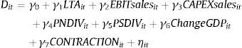
Dit=1 if Dit∗>0 and Dit=0 if Dit∗<0, where Dit∗ is an unobserved latent variable observed as Dit=1 if Dit∗>0 (diversified firm), and equalling zero otherwise (unisegment firm), and ηit is an error term. Independent variables assume that the diversification decision is driven by characteristics10:
- •
at firm-level: firm size (LTA); profitability, approximated by the ratio EBIT to sales (EBITsales); and the firm's level of investment in current operations, proxied by the ratio capital expenditures to total sales (CAPEXsales)
- •
at industry-level: industry attractiveness, based on both the fraction of firms in the firm's core industry that are diversified (PNDIV) and the proportion of the firm's core industry sales accounted for by diversifiers (PSDIV)11
- •
and at the macro-economic level: economic cycle attractiveness, approximated by the real growth rates of gross domestic product, calculated as the GDP percent change based on chained 2005 dollars (changeGDP); and the number of months in the year the U.S. economy was in recession (CONTRACTION).
The selection correction (λi) computed in the first stage of the Heckman procedure is introduced as an additional regressor in the second stage (as shown in the specification of our models indicated above), where outcome equations (1)–(4) are estimated. The significance of λi identifies the presence of selectivity in the sample. In the absence of any selectivity, the correlation (ρ) between the residuals of the selection equation and the outcome equation is close to zero, and the lambda coefficient lacks statistical significance.
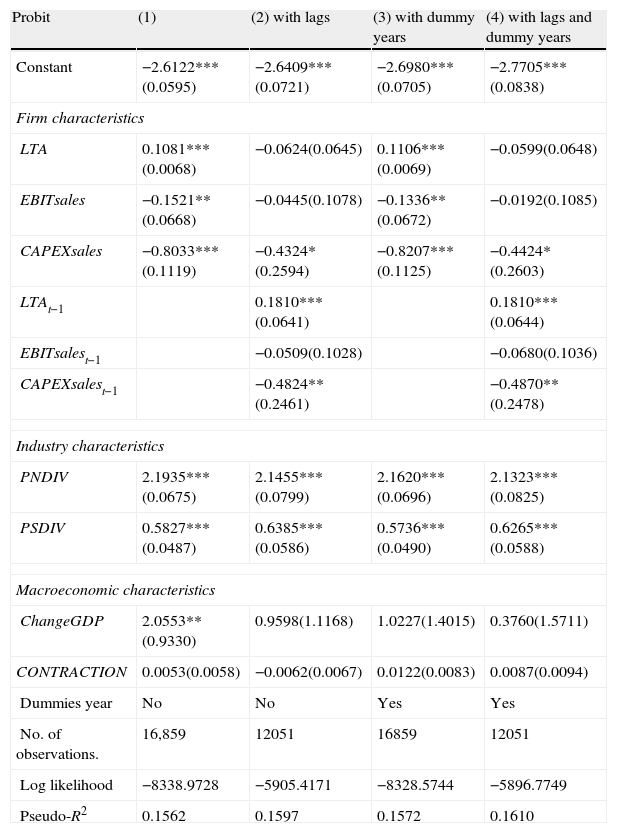
3Empirical findings3.1Heckman first stage: firm propensity to diversifyTable 2 reports the estimations of the selection equation, the first stage of the Heckman procedure (Eq. (5)). Estimations in columns (2)–(4) extend probit specification (1) by incorporating lags and dummy years. The goodness-of-fit (pseudo-R squared) lies in the 0.1562–0.1610 range, comparable to prior literature. Among characteristics at the firm-level, LTA and its lag display a positive and highly significant coefficient (above the 1% level), suggesting that larger enterprises are more likely to engage in diversification. EBITsales is only statistically significant in the models where lagged variables are omitted. Our results reveal that less profitable companies are more liable to diversify. The CAPEXsales variable shows a negative and significant coefficient across all estimations, suggesting that companies with poorer investment are more given to diversify.
Probit model [first stage of the Heckman estimation].
| Probit | (1) | (2) with lags | (3) with dummy years | (4) with lags and dummy years |
| Constant | −2.6122***(0.0595) | −2.6409***(0.0721) | −2.6980***(0.0705) | −2.7705***(0.0838) |
| Firm characteristics | ||||
| LTA | 0.1081***(0.0068) | −0.0624(0.0645) | 0.1106***(0.0069) | −0.0599(0.0648) |
| EBITsales | −0.1521**(0.0668) | −0.0445(0.1078) | −0.1336**(0.0672) | −0.0192(0.1085) |
| CAPEXsales | −0.8033***(0.1119) | −0.4324*(0.2594) | −0.8207***(0.1125) | −0.4424*(0.2603) |
| LTAt−1 | 0.1810***(0.0641) | 0.1810***(0.0644) | ||
| EBITsalest−1 | −0.0509(0.1028) | −0.0680(0.1036) | ||
| CAPEXsalest−1 | −0.4824**(0.2461) | −0.4870**(0.2478) | ||
| Industry characteristics | ||||
| PNDIV | 2.1935***(0.0675) | 2.1455***(0.0799) | 2.1620***(0.0696) | 2.1323***(0.0825) |
| PSDIV | 0.5827***(0.0487) | 0.6385***(0.0586) | 0.5736***(0.0490) | 0.6265***(0.0588) |
| Macroeconomic characteristics | ||||
| ChangeGDP | 2.0553**(0.9330) | 0.9598(1.1168) | 1.0227(1.4015) | 0.3760(1.5711) |
| CONTRACTION | 0.0053(0.0058) | −0.0062(0.0067) | 0.0122(0.0083) | 0.0087(0.0094) |
| Dummies year | No | No | Yes | Yes |
| No. of observations. | 16,859 | 12051 | 16859 | 12051 |
| Log likelihood | −8338.9728 | −5905.4171 | −8328.5744 | −5896.7749 |
| Pseudo-R2 | 0.1562 | 0.1597 | 0.1572 | 0.1610 |
This table shows probit estimation results for the selection equation (Eq. (5)) as the first stage of Heckman's procedure. The dependent variable takes the value 1 when the firm is diversified and zero otherwise. The pseudo-R square indicates the goodness of fit. Standard error is shown in parentheses under coefficients. ****, **, and * denote statistical significance at the 1%, 5%, and 10% level, respectively.
As far as industry variables are concerned, PNDIV and PSDIV are significant by any standards (p-value=0.000). This evidence agrees with Campa and Kedia (2002), and Villalonga (2004b), and indicates that firms are more likely to undertake diversification when there is a stronger presence of diversifiers in the core industry.
Also in line with Campa and Kedia (2002), macroeconomic variables mostly lack statistical significance for explaining the diversification decision. Only ChangeGDP is significant in the probit specification in column (1), and is positively associated with the diversification decision. It yields evidence that companies are more likely to diversify during cycles of economic growth.
Overall, our results suggest that firm and industry characteristics are the key drivers of the diversification decision. At the second stage of the Heckman estimations, we take the probit specification estimated in column (1) of Table 2 to compute the correction for self-selection, λ. Thus, we omit lagged values and year dummies which proved mostly non-significant, while minimizing the loss of observations for subsequent analyses. This probit (1) ensures the existence of at least four exclusion restrictions12 since PNDIV, PSDIV, changeGDP, and CONTRACTION are included in the selection equation but not in the outcome equations, thus mitigating potential collinearity problems.
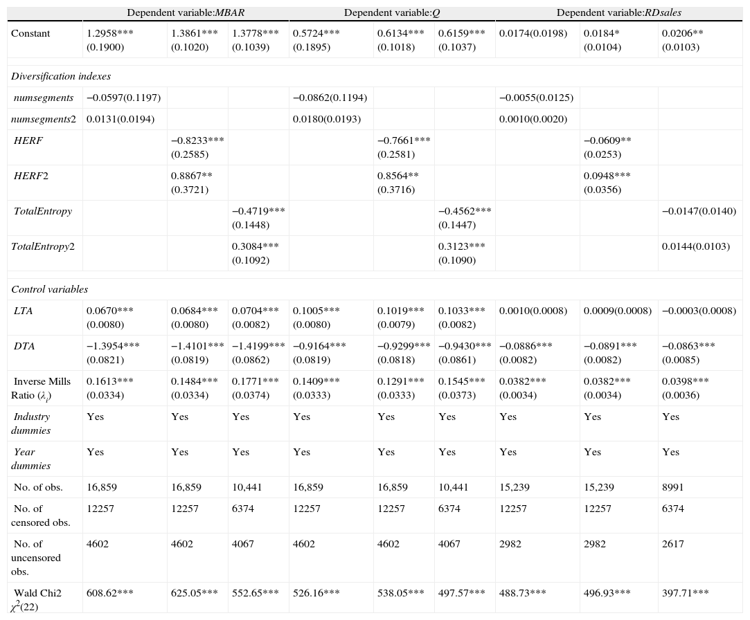
3.2The effect of diversification on GORTable 3 illustrates the Heckman second-stage estimation results of Eq. (1) to check how GOR (proxied by MBAR, Q or RDsales) relates to the degree of diversification (measured by either numsegments, HERF or TotalEntropy), and assess the existence of an effect which may be mediated. Overall, our results provide evidence that the impact of GOR diversification takes a U-form. When numsegments is used to proxy for the diversification scope, this measure and its square contain no statistical significance in any model. This result might be explained by the fact that this proxy based on the simple count of the number of businesses (and thus, not considering the distribution of a firm's total business activity across them) may fail to capture the full extent of diversification.
Diversification level and growth opportunities (Heckman two-step estimator) [Eq. (1)].
| Dependent variable:MBAR | Dependent variable:Q | Dependent variable:RDsales | |||||||
| Constant | 1.2958***(0.1900) | 1.3861***(0.1020) | 1.3778***(0.1039) | 0.5724***(0.1895) | 0.6134***(0.1018) | 0.6159***(0.1037) | 0.0174(0.0198) | 0.0184*(0.0104) | 0.0206**(0.0103) |
| Diversification indexes | |||||||||
| numsegments | −0.0597(0.1197) | −0.0862(0.1194) | −0.0055(0.0125) | ||||||
| numsegments2 | 0.0131(0.0194) | 0.0180(0.0193) | 0.0010(0.0020) | ||||||
| HERF | −0.8233***(0.2585) | −0.7661***(0.2581) | −0.0609**(0.0253) | ||||||
| HERF2 | 0.8867**(0.3721) | 0.8564**(0.3716) | 0.0948***(0.0356) | ||||||
| TotalEntropy | −0.4719***(0.1448) | −0.4562***(0.1447) | −0.0147(0.0140) | ||||||
| TotalEntropy2 | 0.3084***(0.1092) | 0.3123***(0.1090) | 0.0144(0.0103) | ||||||
| Control variables | |||||||||
| LTA | 0.0670***(0.0080) | 0.0684***(0.0080) | 0.0704***(0.0082) | 0.1005***(0.0080) | 0.1019***(0.0079) | 0.1033***(0.0082) | 0.0010(0.0008) | 0.0009(0.0008) | −0.0003(0.0008) |
| DTA | −1.3954***(0.0821) | −1.4101***(0.0819) | −1.4199***(0.0862) | −0.9164***(0.0819) | −0.9299***(0.0818) | −0.9430***(0.0861) | −0.0886***(0.0082) | −0.0891***(0.0082) | −0.0863***(0.0085) |
| Inverse Mills Ratio (λi) | 0.1613***(0.0334) | 0.1484***(0.0334) | 0.1771***(0.0374) | 0.1409***(0.0333) | 0.1291***(0.0333) | 0.1545***(0.0373) | 0.0382***(0.0034) | 0.0382***(0.0034) | 0.0398***(0.0036) |
| Industry dummies | Yes | Yes | Yes | Yes | Yes | Yes | Yes | Yes | Yes |
| Year dummies | Yes | Yes | Yes | Yes | Yes | Yes | Yes | Yes | Yes |
| No. of obs. | 16,859 | 16,859 | 10,441 | 16,859 | 16,859 | 10,441 | 15,239 | 15,239 | 8991 |
| No. of censored obs. | 12257 | 12257 | 6374 | 12257 | 12257 | 6374 | 12257 | 12257 | 6374 |
| No. of uncensored obs. | 4602 | 4602 | 4067 | 4602 | 4602 | 4067 | 2982 | 2982 | 2617 |
| Wald Chi2 χ2(22) | 608.62*** | 625.05*** | 552.65*** | 526.16*** | 538.05*** | 497.57*** | 488.73*** | 496.93*** | 397.71*** |
This table reports the Heckman second stage estimation by OLS (Heckman's two-step estimator) of Eq. (1). The selection equation (column 1) (Table 2) models firms’ propensity to diversify. Different proxies for growth options ratio to the firm's total value (GOR) (either MBAR (the market to book assets ratio), Q (Tobin's Q), or RDsales (the ratio of R&D expenses to firm sales)) are regressed on the degree of diversification. This degree of diversification is proxied by numsegments (number of business segments), HERF (the Herfindahl index) or TotalEntropy (the Total Entropy index), alternatively. Firm size (LTA), financial leverage (DTA), industry effect (Industry dummies), and time effect (Year dummies) are controlled in all estimations. The Inverse Mills Ratio (λi) is included as an additional regressor to correct potential self-selection bias in the sample. The Wald test contrasts the null hypothesis of no joint significance of the explanatory variables. Standard error is shown in parentheses under coefficients. ****, **, and * denote statistical significance at the 1%, 5%, and 10% level, respectively.
However, when the degree of diversification is approximated by more sophisticated indexes such as HERF or TotalEntropy which reflect a broader scope of this strategy, results provide strong evidence (above 1% in most cases) of a U-form relationship with growth opportunities proxies, results being robust across MBAR, Q, and RDsales (in the case of HERF). We calculate the minimum of the curve, our calculations being based on the HERF proxy, which offers the strongest and most robust evidence in our analyses. The critical point HERF* ranges from 0.3212 to 0.4642 across the various estimations. The estimated coefficient associated with λ proves significant above 1% in all regressions (p-value=0.000), confirming the existence of selectivity in our sample. The Wald test indicates that variables are jointly significant.
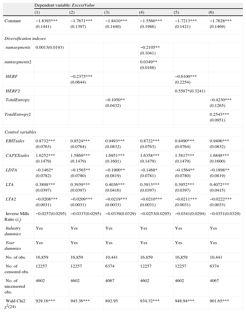
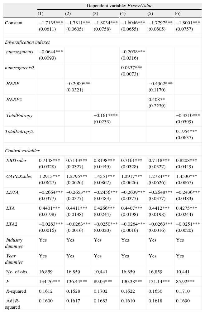
3.3The diversification–value relationshipWe estimate the direct effect of diversification on excess value on Tables 4a and 5a. First, we estimate a linear effect between diversification and excess value (Eq. (2)). Consistent with most prior literature, we find a diversification discount (columns (1)–(3) of Table 4a). Next, we test the presence of a nonlinear effect of diversification on GOR. As reported in columns (4)–(6) of Table 4a, our results reveal a U relation between the ExcessValue and diversification proxies (numsegments, HERF or TotalEntropy) (Eq. (3)), although the lack of any statistical significance in the λ coefficient prevents us obtaining any evidence of selectivity in our sample to fully justify the use of Heckman in this case.
Diversification and excess value (Heckman two-step estimator) [Eqs. (2) and (3)].
| Dependent variable: ExcessValue | ||||||
| (1) | (2) | (3) | (4) | (5) | (6) | |
| Constant | −1.8393***(0.1441) | −1.7671***(0.1397) | −1.8410***(0.1440) | −1.5560***(0.1986) | −1.7213***(0.1421) | −1.7628***(0.1469) |
| Diversification indexes | ||||||
| numsegments | 0.0013(0.0193) | −0.2105**(0.1041) | ||||
| numsegments2 | 0.0349**(0.0168) | |||||
| HERF | −0.2375***(0.0644) | −0.6100***(0.2254) | ||||
| HERF2 | 0.5587*(0.3241) | |||||
| TotalEntropy | −0.1050**(0.0432) | −0.4230***(0.1265) | ||||
| TotalEntropy2 | 0.2543***(0.0951) | |||||
| Control variables | ||||||
| EBITsales | 0.8732***(0.0763) | 0.8524***(0.0764) | 0.9493***(0.0832) | 0.8722***(0.0763) | 0.8490***(0.0764) | 0.9406***(0.0832) |
| CAPEXsales | 1.6252***(0.1479) | 1.5869***(0.1479) | 1.6951***(0.1601) | 1.6358***(0.1479) | 1.5817***(0.1479) | 1.6848***(0.1600) |
| LDTA | −0.1462*(0.0782) | −0.1565**(0.0780) | −0.1900**(0.0819) | −0.1468*(0.0781) | −0.1564**(0.0780) | −0.1898**(0.0819) |
| LTA | 0.3898***(0.0397) | 0.3939***(0.0397) | 0.4036***(0.0416) | 0.3913***(0.0397) | 0.3952***(0.0397) | 0.4072***(0.0415) |
| LTA2 | −0.0208***(0.0031) | −0.0209***(0.0031) | −0.0219***(0.0033) | −0.0210***(0.0031) | −0.0211***(0.0031) | −0.0222***(0.0033) |
| Inverse Mills Ratio (λi) | −0.0257(0.0295) | −0.0337(0.0295) | −0.0339(0.0329) | −0.0253(0.0295) | −0.0341(0.0294) | −0.0351(0.0329) |
| Industry dummies | Yes | Yes | Yes | Yes | Yes | Yes |
| Year dummies | Yes | Yes | Yes | Yes | Yes | Yes |
| No. of obs. | 16,859 | 16,859 | 10,441 | 16,859 | 16,859 | 10,441 |
| No. of censored obs. | 12257 | 12257 | 6374 | 12257 | 12257 | 6374 |
| No. of uncensored obs. | 4602 | 4602 | 4067 | 4602 | 4602 | 4067 |
| Wald Chi2 χ2(24) | 929.16*** | 945.36*** | 892.95 | 934.32*** | 948.94*** | 901.65*** |
This table reports the Heckman second stage estimation by OLS (Heckman's two-step estimator) of Eqs. (2) and (3). The selection equation (column 1) (Table 2) models firms’ propensity to diversify. Columns (1)–(6) contain the Heckman estimation of the direct effect of diversification on ExcessValue. The Excess Value measure developed by Berger and Ofek (1995) is regressed on the degree of diversification (columns (1) to (3)) and its square (columns (4) to (6)). This degree of diversification is proxied by numsegments (number of business segments), HERF (the Herfindahl index), or TotalEntropy (the Total Entropy index), alternatively. Profitability (EBITsales), level of investment in current operations (CAPEXsales), financial leverage (LDTA), firm size (LTA) and its square (LTA2), industry effect (Industry dummies), and time effect (Year dummies) are controlled in all estimations. The Inverse Mills Ratio (λi) is included as an additional regressor to correct potential self-selection bias in the sample. The Wald test contrasts the null hypothesis of no joint significance of the explanatory variables. Standard error is shown in parentheses under coefficients. ****, **, and * denote statistical significance at the 1%, 5%, and 10% level, respectively.
Diversification and excess value (OLS) [Eqs. (2) and (3)].
| Dependent variable: ExcessValue | ||||||
| (1) | (2) | (3) | (4) | (5) | (6) | |
| Constant | −1.7135***(0.0611) | −1.7811***(0.0605) | −1.8034***(0.0758) | −1.6046***(0.0655) | −1.7797***(0.0605) | −1.8001***(0.0757) |
| Diversification indexes | ||||||
| numsegments | −0.0644***(0.0093) | −0.2038***(0.0316) | ||||
| numsegments2 | 0.0337***(0.0073) | |||||
| HERF | −0.2909***(0.0321) | −0.4962***(0.1170) | ||||
| HERF2 | 0.4087*(0.2239) | |||||
| TotalEntropy | −0.1617***(0.0233) | −0.3310***(0.0599) | ||||
| TotalEntropy2 | 0.1954***(0.0637) | |||||
| Control variables | ||||||
| EBITsales | 0.7148***(0.0328) | 0.7113***(0.0327) | 0.8198***(0.0449) | 0.7161***(0.0328) | 0.7118***(0.0327) | 0.8208***(0.0449) |
| CAPEXsales | 1.2913***(0.0627) | 1.2795***(0.0626) | 1.4551***(0.0867) | 1.2917***(0.0626) | 1.2784***(0.0626) | 1.4530***(0.0867) |
| LDTA | −0.2664***(0.0377) | −0.2653***(0.0377) | −0.2456***(0.0483) | −0.2639***(0.0377) | −0.2648***(0.0377) | −0.2436***(0.0483) |
| LTA | 0.4401***(0.0198) | 0.4411***(0.0198) | 0.4266***(0.0244) | 0.4407***(0.0198) | 0.4412***(0.0198) | 0.4275***(0.0244) |
| LTA2 | −0.0263***(0.0016) | −0.0263***(0.0016) | −0.0250***(0.0020) | −0.0264***(0.0016) | −0.0263***(0.0016) | −0.0251***(0.0020) |
| Industry dummies | Yes | Yes | Yes | Yes | Yes | Yes |
| Year dummies | Yes | Yes | Yes | Yes | Yes | Yes |
| No. of obs. | 16,859 | 16,859 | 10,441 | 16,859 | 16,859 | 10,441 |
| F | 134.76*** | 136.44*** | 89.03*** | 130.38*** | 131.14*** | 85.92*** |
| R-squared | 0.1612 | 0.1628 | 0.1702 | 0.1622 | 0.1630 | 0.1710 |
| Adj R-squared | 0.1600 | 0.1617 | 0.1683 | 0.1610 | 0.1618 | 0.1690 |
This table reports the OLS regressions of Eqs. (2) and (3). The ExcessValue measure developed by Berger and Ofek (1995) is regressed on the level of diversification (columns (1) to (3)) and its square (columns (4) to (6)). This degree of diversification is proxied by numsegments (number of business segments), HERF (the Herfindahl index) or TotalEntropy (the Total Entropy index), alternatively. Profitability (EBITsales), level of investment in current operations (CAPEXsales), financial leverage (LDTA), firm size (LTA) and its square (LTA2), industry effect (Industry dummies), and time effect (Year dummies) are controlled in all estimations. The F test contrasts the null hypothesis of no joint significance of the explanatory variables. R-squared measures the goodness of fit. Standard error is shown in parentheses under coefficients. ****, **, and * denote statistical significance at the 1%, 5%, and 10% level, respectively.
Alternatively, columns (4)–(6) of Table 5a contain the OLS estimations which also support this quadratic relationship, with even stronger statistical significance. In the early stages of diversification, diversified firms trade at a discount relative to unisegment firms until a critical point is reached (located at numsegments*=3.023713; HERF*=0.6070) from which the value outcomes of this strategy become positive. Thus, at diversification levels below this minimum, and as found in most prior papers, diversification tends to trade at a discount. However, from this point, the relationship may flip, and it may be possible to obtain a diversification premium, as supported in recent papers.
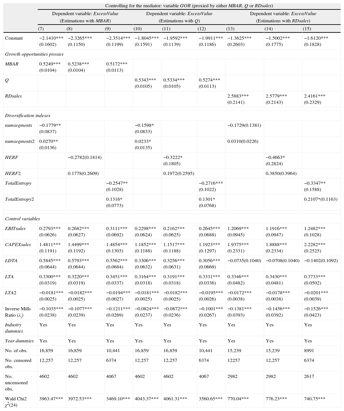
3.4The mediating effect of GOR in the diversification–value relationshipHaving confirmed the U relation linking diversification and GOR, and diversification and ExcessValue, we go one step further to examine whether such a curvilinear effect is driven by GOR. We need to check whether GOR acts as a mediator in the diversification–value relationship. Should this be the case, the impact of the degree of diversification on ExcessValue would weaken or lose its statistical significance once growth opportunities are included in the model. Table 4b displays the Heckman two-step estimations of Eq. (4).
Heckman regression analysis of the mediating role of GOR in the diversification-value relationship (Heckman two-step estimator) [Eq. (4)].
| Controlling for the mediator: variable GOR (proxied by either MBAR, Q or RDsales) | |||||||||
| Dependent variable: ExcessValue | Dependent variable: ExcessValue | Dependent variable: ExcessValue | |||||||
| (Estimations with MBAR) | (Estimations with Q) | (Estimations with RDsales) | |||||||
| (7) | (8) | (9) | (10) | (11) | (12) | (13) | (14) | (15) | |
| Constant | −2.1410***(0.1602) | −2.3265***(0.1150) | −2.3514***(0.1199) | −1.8045***(0.1591) | −1.9592***(0.1139) | −1.9911***(0.1186) | −1.3625***(0.2603) | −1.5002***(0.1775) | −1.6120***(0.1828) |
| Growth opportunities proxies | |||||||||
| MBAR | 0.5249***(0.0104) | 0.5238***(0.0104) | 0.5172***(0.0113) | ||||||
| Q | 0.5343***(0.0105) | 0.5334***(0.0105) | 0.5274***(0.0113) | ||||||
| RDsales | 2.5883***(0.2141) | 2.5779***(0.2143) | 2.4161***(0.2329) | ||||||
| Diversification indexes | |||||||||
| numsegments | −0.1779**(0.0837) | −0.1598*(0.0833) | −0.1729(0.1381) | ||||||
| numsegments2 | 0.0270**(0.0136) | 0.0233*(0.0135) | 0.0310(0.0226) | ||||||
| HERF | −0.2782(0.1814) | −0.3222*(0.1805) | −0.4663*(0.2824) | ||||||
| HERF2 | 0.1778(0.2609) | 0.1972(0.2595) | 0.3850(0.3964) | ||||||
| TotalEntropy | −0.2547**(0.1028) | −0.2716***(0.1022) | −0.3347**(0.1588) | ||||||
| TotalEntropy2 | 0.1316*(0.0773) | 0.1301*(0.0768) | 0.2107*(0.1163) | ||||||
| Control variables | |||||||||
| EBITsales | 0.2793***(0.0626) | 0.2682***(0.0627) | 0.3111***(0.0692) | 0.2298***(0.0624) | 0.2162***(0.0625) | 0.2645***(0.0688) | 1.2069***(0.0945) | 1.1916***(0.0947) | 1.2482***(0.1028) |
| CAPEXsales | 1.4811***(0.1191) | 1.4499***(0.1192) | 1.4854***(0.1303) | 1.1852***(0.1188) | 1.1517***(0.1188) | 1.1923***(0.1297) | 1.9375***(0.2331) | 1.8888***(0.2334) | 2.2282***(0.2525) |
| LDTA | 0.5845***(0.0644) | 0.5793***(0.0644) | 0.5562***(0.0684) | 0.3306***(0.0632) | 0.3256***(0.0631) | 0.3056***(0.0669) | −0.0735(0.1040) | −0.0708(0.1040) | −0.1402(0.1092) |
| LTA | 0.3300***(0.0319) | 0.3220***(0.0319) | 0.3451***(0.0337) | 0.3164***(0.0318) | 0.3191***(0.0318) | 0.3331***(0.0336) | 0.3346***(0.0482) | 0.3430***(0.0481) | 0.3733***(0.0502) |
| LTA2 | −0.0181***(0.0025) | −0.0182***(0.0025) | −0.0194***(0.0027) | −0.0181***(0.0025) | −0.0182***(0.0025) | −0.0195***(0.0026) | −0.0172***(0.0038) | −0.0178***(0.0038) | −0.0201***(0.0039) |
| Inverse Mills Ratio (λi) | −0.1035***(0.0238) | −0.1077***(0.0239) | −0.1211***(0.0269) | −0.0824***(0.0237) | −0.0872***(0.0236) | −0.1001***(0.0267) | −0.1381***(0.0393) | −0.1456***(0.0392) | −0.1526***(0.0423) |
| Industry dummies | Yes | Yes | Yes | Yes | Yes | Yes | Yes | Yes | Yes |
| Year dummies | Yes | Yes | Yes | Yes | Yes | Yes | Yes | Yes | Yes |
| No. of obs. | 16,859 | 16,859 | 10,441 | 16,859 | 16,859 | 10,441 | 15,239 | 15,239 | 8991 |
| No. censored obs. | 12,257 | 12,257 | 6374 | 12,257 | 12,257 | 6374 | 12257 | 12,257 | 6374 |
| No. uncensored obs. | 4602 | 4602 | 4067 | 4602 | 4602 | 4067 | 2982 | 2982 | 2617 |
| Wald Chi2 χ2(24) | 3963.47*** | 3972.53*** | 3469.10*** | 4043.37*** | 4061.31*** | 3560.65*** | 770.04*** | 776.23*** | 740.75*** |
This table reports the Heckman second stage estimation by OLS (Heckman's two−step estimator) of the analysis of the mediating effect of GOR in the diversification-value relationship (Eq. (4)). The selection equation (column 1) (Table 2) models firms’ propensity to diversify. Columns (7)–(15) display the Heckman estimation of ExcessValue measure developed by Berger and Ofek (1995) on both the diversification variables and the GOR proxies. The degree of diversification is proxied by numsegments (number of business segments), HERF (the Herfindahl index) or TotalEntropy (the Total Entropy index), alternatively. Different proxies for GOR (either MBAR (the market to book assets ratio), Q (Tobin's Q) or RDsales (the ratio of R&D expenses to firm sales)) are used. Profitability (EBITsales), level of investment in current operations (CAPEXsales), financial leverage (LDTA), firm size (LTA) and its square (LTA2), industry effect (Industry dummies), and time effect (Year dummies) are controlled in all estimations. The Inverse Mills Ratio (λi) is included as an additional regressor to correct potential self-selection bias in the sample. The Wald test contrasts the null hypothesis of no joint significance of the explanatory variables. Standard error is shown in parentheses under coefficients. ****, **, and * denote statistical significance at the 1%, 5%, and 10% level, respectively.
As shown in Table 4b, our data confirm a positive and strongly significant statistical relationship (p-value=0.000) between the proxies for growth opportunities (either MBAR, Q or RDsales) and ExcessValue. Contrary to Stowe and Xing (2006), we find that a firm's set of growth opportunities significantly account for the diversification value outcomes. Our empirical findings suggest that the larger the fraction represented by growth opportunities over the firm's total value, the higher the ExcessValue and thus the lower the discount (or the greater the premium). This finding is consistent with prior works such as Ferris et al. (2002).
Our results also provide evidence supporting partial mediation. When GOR is accounted for, the coefficients associated with the quadratic term of diversification reduce their statistical significance, which is even lost in the regressions on the HERF proxy. These findings suggest that GOR is partially mediating the U-effect between diversification and ExcessValue.
In sum, growth opportunities play a relevant role in explaining the U-form function linking diversification and ExcessValue, making this corporate strategy less value-destroying after a certain level of diversification. This may be due to two reasons: firstly, because the critical points of the curve linking the degree of diversification and GOR and the one relating diversification to ExcessValue are not too far away from each other (the former being lower than the latter), suggesting in some way that this strategy becomes more beneficial at stages when a broader extent of diversification mainly serves as a platform for further growth opportunities; and secondly, because when GOR is included in the regression of ExcessValue on diversification, the quadratic term of DIVER reduces its statistical significance (which is particularly noticeable when HERF or TotalEntropy are used).
3.5Additional robustness checksWe conduct further robustness analyses. Firstly, we re-estimate all equations by an alternative procedure, the Heckman maximum likelihood (ML) estimator.14 Secondly, we winsorize the top and bottom 5.98% of ExcessValue to reduce the effect of ‘extreme’ excess values (above 1.386 or below −1.386) (Berger and Ofek, 1995). Analyses involving Eq. (2)–(4) are then re-estimated using the winsorized variable (wExcessValue) as a dependent variable.15 Our findings persist through these robustness tests.
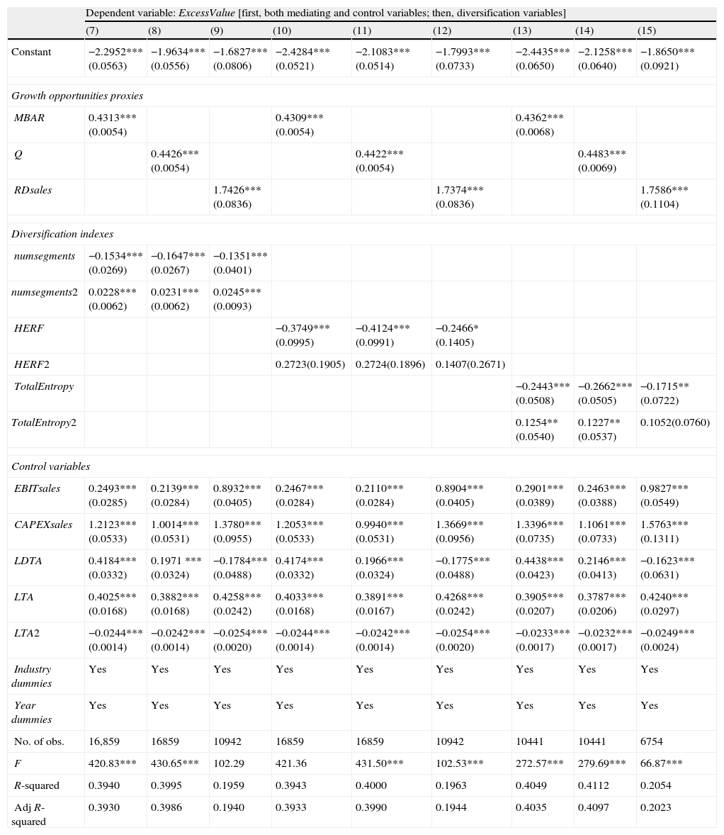
In addition, in testing the mediating effect, we follow Hill and Snell (1988), and re-estimate Eq. (4) using hierarchical regression techniques.16 This methodology estimates Eq. (4) in which GOR enters first, followed by DIVER to evaluate whether any previous significant relationship between DIVER and ExcessValue loses significance when considering GOR. See Table 5b for a summary of the results.
Hierarchical regression analyses of the mediating role of GOR in the diversification-value relationship (OLS) [Eq. (4)].
| Dependent variable: ExcessValue [first, both mediating and control variables; then, diversification variables] | |||||||||
| (7) | (8) | (9) | (10) | (11) | (12) | (13) | (14) | (15) | |
| Constant | −2.2952***(0.0563) | −1.9634***(0.0556) | −1.6827***(0.0806) | −2.4284***(0.0521) | −2.1083***(0.0514) | −1.7993***(0.0733) | −2.4435***(0.0650) | −2.1258***(0.0640) | −1.8650***(0.0921) |
| Growth opportunities proxies | |||||||||
| MBAR | 0.4313***(0.0054) | 0.4309***(0.0054) | 0.4362***(0.0068) | ||||||
| Q | 0.4426***(0.0054) | 0.4422***(0.0054) | 0.4483***(0.0069) | ||||||
| RDsales | 1.7426***(0.0836) | 1.7374***(0.0836) | 1.7586***(0.1104) | ||||||
| Diversification indexes | |||||||||
| numsegments | −0.1534***(0.0269) | −0.1647***(0.0267) | −0.1351***(0.0401) | ||||||
| numsegments2 | 0.0228***(0.0062) | 0.0231***(0.0062) | 0.0245***(0.0093) | ||||||
| HERF | −0.3749***(0.0995) | −0.4124***(0.0991) | −0.2466*(0.1405) | ||||||
| HERF2 | 0.2723(0.1905) | 0.2724(0.1896) | 0.1407(0.2671) | ||||||
| TotalEntropy | −0.2443***(0.0508) | −0.2662***(0.0505) | −0.1715**(0.0722) | ||||||
| TotalEntropy2 | 0.1254**(0.0540) | 0.1227**(0.0537) | 0.1052(0.0760) | ||||||
| Control variables | |||||||||
| EBITsales | 0.2493***(0.0285) | 0.2139***(0.0284) | 0.8932***(0.0405) | 0.2467***(0.0284) | 0.2110***(0.0284) | 0.8904***(0.0405) | 0.2901***(0.0389) | 0.2463***(0.0388) | 0.9827***(0.0549) |
| CAPEXsales | 1.2123***(0.0533) | 1.0014***(0.0531) | 1.3780***(0.0955) | 1.2053***(0.0533) | 0.9940***(0.0531) | 1.3669***(0.0956) | 1.3396***(0.0735) | 1.1061***(0.0733) | 1.5763***(0.1311) |
| LDTA | 0.4184***(0.0332) | 0.1971 ***(0.0324) | −0.1784***(0.0488) | 0.4174***(0.0332) | 0.1966***(0.0324) | −0.1775***(0.0488) | 0.4438***(0.0423) | 0.2146***(0.0413) | −0.1623***(0.0631) |
| LTA | 0.4025***(0.0168) | 0.3882***(0.0168) | 0.4258***(0.0242) | 0.4033***(0.0168) | 0.3891***(0.0167) | 0.4268***(0.0242) | 0.3905***(0.0207) | 0.3787***(0.0206) | 0.4240***(0.0297) |
| LTA2 | −0.0244***(0.0014) | −0.0242***(0.0014) | −0.0254***(0.0020) | −0.0244***(0.0014) | −0.0242***(0.0014) | −0.0254***(0.0020) | −0.0233***(0.0017) | −0.0232***(0.0017) | −0.0249***(0.0024) |
| Industry dummies | Yes | Yes | Yes | Yes | Yes | Yes | Yes | Yes | Yes |
| Year dummies | Yes | Yes | Yes | Yes | Yes | Yes | Yes | Yes | Yes |
| No. of obs. | 16,859 | 16859 | 10942 | 16859 | 16859 | 10942 | 10441 | 10441 | 6754 |
| F | 420.83*** | 430.65*** | 102.29 | 421.36 | 431.50*** | 102.53*** | 272.57*** | 279.69*** | 66.87*** |
| R-squared | 0.3940 | 0.3995 | 0.1959 | 0.3943 | 0.4000 | 0.1963 | 0.4049 | 0.4112 | 0.2054 |
| Adj R-squared | 0.3930 | 0.3986 | 0.1940 | 0.3933 | 0.3990 | 0.1944 | 0.4035 | 0.4097 | 0.2023 |
This table reports the hierarchical estimations of the analysis of the mediating role of GOR in the diversification-value relationship (Eq. (4)). Columns (7)–(15) display the OLS estimations of the ExcessValue measure developed by Berger and Ofek (1995) on both the diversification variables and the GOR proxies, in which the GOR proxy is entered first. The degree of diversification is proxied by numsegments (number of business segments), HERF (the Herfindahl index) or TotalEntropy (the Total Entropy index), alternatively. Different proxies for GOR (either MBAR (the market to book assets ratio), Q (Tobin's Q) or RDsales (the ratio of R&D expenses to firm sales)) are used. Profitability (EBITsales), level of investment in current operations (CAPEXsales), financial leverage (LDTA), firm size (LTA) and its square (LTA2), industry effect (Industry dummies), and time effect (Year dummies) are controlled in all estimations. The F test contrasts the null hypothesis of no joint significance of the explanatory variables. R-squared measures the goodness of fit. Standard error is shown in parentheses under coefficients. ***, **, and * denote statistical significance at the 1%, 5%, and 10% level, respectively.
Our results remain robust to hierarchical regressions. When using HERF and TotalEntropy as proxies for diversification, results reveal that growth opportunities partially mediate the relationship between diversification and ExcessValue. In particular, the coefficient associated with the quadratic term of diversification declines in statistical significance in regressions containing TotalEntropy and even becomes non-significant when HERF approximates diversification. Evidence is stronger in the case of the RDsales proxy as the significance of the two coefficients associated with the diversification variables decreases. In the case of numsegments, we find no evidence of a partially mediated effect, since the significance of the diversification variables remains equally strong even when GOR proxies are entered first. Results hold after replacing ExcessValue by wExcessValue as the dependent variable.15
4ConclusionThis paper contributes to the literature by providing further empirical evidence on the diversification–value relationship. Our results suggest a U-shaped effect of diversification on a firm's value and support a partial mediating role of growth opportunities on this relationship.
Specifically, our data shows that at its lower levels, diversification has a negative effect on a firm's market value, resulting in a diversification discount. However, at high levels of diversification, said negative relationship between diversification and value turns around and becomes positive. We report evidence suggesting that this finding may be explained by growth opportunities. We find a U-shaped relationship between the level of diversification and the portion of a firm's market value which is accounted for by its growth opportunities. This evidence of a quadratic relationship between diversification and GOR may be logically interpreted as indicating that, in the early stages of diversification, investing in a new business mainly involves replacing growth opportunities by assets in place, while in its later stages diversification becomes a net source of further growth options. This latter effect may be due to the progressive accumulation of knowledge and capabilities arising from simultaneously taking part in several businesses, which improves a firm's ability to sense and seize opportunities in a wider range of industries. Moreover, as the firm spreads its capabilities across alternative businesses, further growth opportunities are more likely to be embedded in those investments.
Additionally, we find that the U-shaped relationship between diversification and GOR carries over partially to the effect of diversification on ExcessValue. This result is consistent with prior research such as Bernardo and Chowdhry (2002) and Ferris et al. (2002), who find that growth opportunities account for part of the diversification discounts/premiums. However, we report evidence of a mediating role of GOR on the U-shaped relation between diversification and firm value, suggesting that the effect of diversification on GOR explains in part how diversification may create or destroy value.
According to Amihud and Lev (1981), diversification creates value in so far as it cannot be replicated at a lower cost by investors. Our results show that at a higher level of diversification GOR experiences a parallel increase with diversification. This makes corporate diversification less attainable by investors in their individual portfolios since they cannot replicate the optimal exercise policy of a set of growth opportunities as a whole, thus giving rise to a premium. This result is consistent with prior literature such as Raynor (2002), who argues that growth options-oriented strategies provide a ‘strategic insurance’ and reduce firm-specific risk in a way investors cannot replicate.
Our study suffers from certain limitations and suggests interesting avenues for future research. The data is collected from a single country. More extensive analyses could be performed on an international setting. In addition, our results leave the door open for other possible mediating variables in the diversification-performance relationship. It might be interesting to explore whether there are additional mediators which might provide a deeper insight into the conditions under which this strategy may be implemented more successfully by companies. Certain theoretical frameworks such as the real options approach, which has a close link to a firm's growth opportunities and its specific resources and capabilities, may become a helpful guide for future research.
Financial support has been received from the Regional Government of Castilla y León (Ref. VA 291 B11-1) and the Spanish Ministry of Science and Innovation (Ref. ECO 2011-29144-C03-01 and ECO2012-32554). Pilar Velasco also acknowledges the financial support from the Spanish Ministry of Education (FPU fellowship).
“But is there an optimum degree of diversification? It is a question many of our clients ask us (advisers at the Boston Consulting Group)” (Heuskel et al., 2006).
Industry segment data at the 4-digit SIC code level.
This body belongs to the U.S. Department of Commerce: http://www.bea.gov/national/index.htm .
See Berger and Ofek (1995) for more details about sample selection.
These proportions are similar to those reported by prior works such as Villalonga (2004b).
We drop observations beyond three standard deviations from the sample mean for each variable.
The U.S. Department of Labor major industries classification: http://www.osha.gov/pls/imis/sic_manual.html.
See Berger and Ofek for a detailed explanation of the calculation of the excess value. We calculate the firm's imputed value based on sales multipliers due to the greater availability of data of sales at the segment-level in Worldscope. Consistent with most prior literature, we estimate a firm's market value (MV) as the sum of market value of equity (MVE), long-term (LtD), short-tem (StD) debt, and preferred stock (PrefStock) (Campa and Kedia, 2002).
Sample selection arises when a random sample is not observed but when the sample observation selection is not independent of the outcome variables (Winship and Mare, 1992). Selectivity has been the subject of intensive research (especially in the labor economics field) since, if not appropriately controlled, it causes bias in results.
See Campa and Kedia (2002) for a further explanation of variables selection.
We calculate these two proxies at the 4-digit SIC level.
The Heckman approach requires at least one variable included in the selection equation but not contained in the outcome equation (Puhani, 2000). The lack of exclusion restrictions is likely to give rise to collinearity problems and the Heckman estimator performs poorly in this case.
In this case, we calculate the minimum taking the numsegments proxy since it is statistically significant and is easier to interpret. We also include the minimum in terms of HERF to allow comparability with our analyses of Eq. (1).
Results are available upon request from the corresponding author. Whereas in the Heckman two-step estimator, the selection equation and the outcome equation are estimated separately by probit and OLS estimations, respectively, in the Heckman ML estimator, both equations are estimated jointly in a single step by maximum likelihood. Assumptions for applying this ML approach are more restrictive than those required by the Heckman two-step estimator.

