


This paper focuses primarily on aggregate default and illiquidity in the credit default swap (CDS) market. We examine how changes in aggregate default and illiquidity are related to changes in spreads of CDS portfolios sorted by credit quality and maturity. We document that aggregate default and liquidity are important determinants of CDS spreads. The default and illiquidity CDS betas across credit quality portfolios and maturities are positive and statistically significant. Low credit rating CDS spreads are highly sensitive to aggregate default and illiquidity shocks relative to high credit quality CDS spreads.
There has been a growing interest in studying liquidity of CDS spreads in addition to default. In efficient markets, spreads of CDS contracts should account for default risk of companies that they reference. However, if markets are not efficient, market frictions give rise to illiquidity. The empirical evidence supports the existence of market frictions in CDS markets (see, for instance, Acharya and Johnson, 2007; Brunnermeier and Pedersen, 2009). Furthermore, the concerns over the default and illiquidity of CDS spreads have become especially relevant after the financial crisis of 2007 when both default and illiquidity skyrocketed jointly.
The main objective of this paper is to analyze the sensitivity of aggregate CDS spreads to market-wide default and illiquidity shocks. The key results of this work are as follows. We show that aggregate liquidity and default spreads are powerful determinants of CDS spreads. There is a consistently positive and significant relationship between CDS spreads and aggregate illiquidity and default spread changes across all maturities and credit qualities. These results suggest that CDS spreads cannot be regarded as a pure measure of creditworthiness of underlying companies as previously reviewed in the CDS literature.1 We also document a monotonic relationship between the sensitivity of both liquidity and credit ratings to market-wide changes, particularly for high-yield underlyings. Our proposed factors on average explain 60% of the variation in aggregate CDS spreads. To the best of our knowledge, this is the first study to address empirically the importance of both default and illiquidity of CDS spreads at an aggregate level.
We conduct the empirical analysis at an aggregate level for two reasons. First, there have been studies finding evidence for commonality in liquidity in bond markets.2 Because CDS markets reference bond markets, CDS markets can also be exposed to market-wide movements in default and illiquidity. Second, we can obtain more precise estimates if we conduct the empirical analysis at an aggregate, rather than individual, level. To sum up, the aggregation is done at a CDS portfolio level sorted by credit quality and maturity. Credit ratings provide a real-world measure of default for underlying CDS companies. On the other hand, if the maturity of CDS contracts is correlated with the volume of CDS trades, the CDS maturity proxies the true unobserved CDS illiquidity.3 Hence, conducting our empirical analyses for credit-quality-sorted portfolios for different maturities can allow us to differentiate the effect of aggregate default on CDS spreads, from the effect of aggregate illiquidity on CDS spreads. We further choose and/or calculate market-wide factors that in theory should explain aggregate CDS spreads in addition to aggregate default and illiquidity. We employ monthly observations of 284 US corporate default swap names from 2004 to 2011. We then perform several regression analyses to study the relative contribution of the market-wide illiquidity and default spread changes to CDS portfolio changes. To guarantee the robustness of our results, we set different controls for credit and macroeconomic risks. In addition, we remove potentially confounding credit risk exposure from the CDS bid-ask spreads.
This work closely follows several studies focusing on liquidity of CDS spreads. Particularly, our empirical results support and complement the analysis of Tang and Yan (2008), Bongaerts et al. (2011), and Buhler and Trapp (2009). Tang and Yan (2008) construct several liquidity proxies to capture various facets of CDS liquidity. They find that liquidity premium and liquidity risk are priced in CDS spreads. Rather than conducting the empirical analysis for a set of individual CDS assets, we complement Tang and Yan (2008) and carry out our analysis for CDS portfolios sorted by credit quality and maturity. Bongaerts et al. (2011) build on the CAPM model of Acharya and Pedersen (2005) and derive an equilibrium asset pricing model that incorporates liquidity risk and short-selling due to hedging of nontraded risk. They estimate their asset pricing model for the credit default swap market and find that expected CDS returns contain significant compensation for both expected liquidity and liquidity risk. To note, both Tang and Yan (2008) and Bongaerts et al. (2011) rely on 5-year CDS spreads for their analysis. Furthermore, they consider the time period before March 2006 and December 2008, respectively. We employ CDS spreads with five different maturities in our empirical analysis and consider the time period up to April 2011, which includes major sovereign credit events since the collapse of Lehman Brothers in September 2008. Buhler and Trapp (2009) develop a reduced form model, which allows them to decompose bond and CDS spreads into a credit risk component, a liquidity component, and a component that measures the relationship between credit risk and liquidity in both bond and CDS markets. Our paper also acknowledges the fact that illiquidity dries up when credit risk increases. Hence, in our empirical analysis we work with a residual measure of illiquidity that is net of default exposure.
Overall, this article analyzes the relevance of market-wide illiquidity and default for aggregate CDS spreads. The paper is organized as follows. Section 2 describes the data employed in the empirical analysis and the methodology for constructing the CDS portfolios. Section 3 provides the empirical results by analyzing the sensitivity of the portfolio CDS spread (sorted by maturity and credit quality) to market-wide illiquidity and default shocks. Section 4 concludes.
2Data, dependent, and explanatory variablesWe collect our sample of CDS spreads from Market. We employ the CDS contracts from North America for which we can obtain the CDS spreads with maturities of either 1, 3, 5, 7, or 10 years from January 2004 to April 2011. We further restrict our sample to corporate CDS names. In addition, we consider CDS contracts that are denominated in US dollars, are written on senior unsecured debt of underlying companies, and include the modified restructuring as a credit event. To obtain the time series of monthly CDS spreads of a given CDS name, we take the last daily CDS spreads for each month and maturity. In total, we have 284 CDS contracts in our sample.
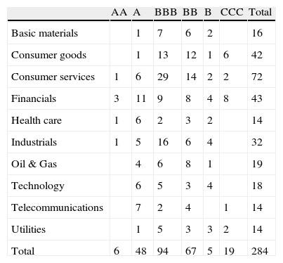
Table 1 provides the distribution of CDS names in our sample by sector and rating group. The reported rating is the resulting average of the Moody's and S&P ratings, adjusted to the seniority of the instrument and rounded so as not to include the plus and minus levels. Markit uses 10-sector ICB classification and adds one additional category for Government. Those sectors are Financial, Oil & Gas, Basic Materials, Industrial, Consumer Goods, Consumer Services, Health Care, Telecommunications, Utilities, Technology and Government. Nearly 52% of the CDS contracts in our database are written on the debt of investment grade companies, while the remaining share of CDS contracts (48%) are written on the debt of high-yield companies. There are four industries individually represented by more than 10% of the total number of contracts. These CDS contracts are written on the debt of companies from the Consumer Services, Financial, Consumer Goods, and Industrial sectors. These four sectors constitute approximately 65% of our sample.
CDS names by sector and rating.
| AA | A | BBB | BB | B | CCC | Total | |
| Basic materials | 1 | 7 | 6 | 2 | 16 | ||
| Consumer goods | 1 | 13 | 12 | 1 | 6 | 42 | |
| Consumer services | 1 | 6 | 29 | 14 | 2 | 2 | 72 |
| Financials | 3 | 11 | 9 | 8 | 4 | 8 | 43 |
| Health care | 1 | 6 | 2 | 3 | 2 | 14 | |
| Industrials | 1 | 5 | 16 | 6 | 4 | 32 | |
| Oil & Gas | 4 | 6 | 8 | 1 | 19 | ||
| Technology | 6 | 5 | 3 | 4 | 18 | ||
| Telecommunications | 7 | 2 | 4 | 1 | 14 | ||
| Utilities | 1 | 5 | 3 | 3 | 2 | 14 | |
| Total | 6 | 48 | 94 | 67 | 5 | 19 | 284 |
This table shows the distribution of CDS names in our database by rating and ICB Industry category. The rating is the average of the Moody's and S&P ratings that are adjusted to the seniority of the instrument and are rounded not to include the plus and minus levels.
Fig. 1 displays the time series of the aggregate monthly CDS spreads by maturity. These series are calculated by taking the cross-sectional average of the individual CDS spreads for each month and maturity. We observe that the CDS spreads of all maturities are relatively stable before mid-2007. After this point, there is a sharp increase in CDS spreads until the beginning of 2009. The dramatic increase in mid-2007 is associated with the housing bubble burst in the US and the associated losses on subprime mortgage asset-backed securities, collateralized bond obligations, and CDSs on the asset-backed holdings. When these financial securities lost value due to the housing market crash, the financial institutions utilizing these products had insufficient capital to respond to the enormous realized losses. Specifically, the upward-sloping trend of CDS spread time series is followed by a series of significant credit events such as the collapse of Lehman Brothers, the bailout of AIG and the federal takeover of Fannie Mae and Freddie Mac in September 2008.4 The slope of the term structure of the CDS spreads is mostly positive, indicating that the spreads of short maturity horizons tend to be lower than the spreads of longer horizons. However, Fig. 1 also shows that from mid-2008 until mid-2009, the CDS spreads with short-term maturity are higher than those with long-term maturity. This inversion of the term structure slope during stress periods has also been documented by Pan and Singleton (2008) for emerging countries during periods of financial or political crisis. It is important to note that the inversion of the slope is perfectly monotonic.5

Time series of sample mean CDS spreads. This graph plots the monthly time series of CDS spreads by maturity. The time series of monthly CDS spreads for each maturity is constructed by taking the cross-sectional average of CDS spreads for each month and maturity. The time period of our sample extends from January 2004 to April 2011.
Our dependent variables in the regression analysis are for portfolios sorted by the credit quality of underlying CDS companies and CDS maturities. The procedure for constructing CDS portfolios is similar to the one employed by Arakelyan et al. (2013). Below we summarize the main steps of their methodology. We form four credit-quality-sorted portfolios of CDS spreads: AAA to A−, BBB+ to BBB−, BB+ to BB−, and B+ to D. More specifically, for each month we allocate the CDS contracts in our sample to these 4 portfolios based on the credit ratings of the underlying CDS names. We obtain the data on credit ratings from Thomson Reuters 3000 Xtra. We consider only long-term issuer rating assigned by S&P, Fitch and Moody's. The observed credit ratings of underlying CDS names are unevenly distributed over time. Yet, for each CDS name we generate a monthly time series of credit ratings, where each monthly observation is a composite average of credit ratings assigned by the three credit agencies. Given that for each underlying CDS company we have the data on the term structure of CDS spreads with 1, 3, 5, 7, and 10 year maturity, overall we obtain 20 time series of portfolio CDS spreads.6 Finally, we equally weigh the CDS spreads in each portfolio. For more details, see Arakelyan et al. (2013).
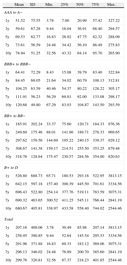
Table 2 reports the summary statistics of CDS spreads of portfolios sorted by credit quality and maturity. Within each credit-quality-sorted portfolio, the CDS spreads increase (on average) as the maturity of the portfolio increases. The same pattern holds for the portfolios sorted only by maturity (bottom panel of Table 2). If we hold the portfolio maturity constant, the CDS spreads increase (on average) with the credit quality of the portfolio, i.e. as the portfolio becomes riskier, the portfolio CDS spread increases. We can draw similar conclusions based on the summary statistics of different percentiles (25%, 50%, and 75%) of CDS spreads sorted by credit quality and maturity. Last but not least, the volatility of CDS portfolios decreases with the maturity holding the credit quality of the portfolio constant, while the volatility seems to increase for high-yield portfolios as we fix the portfolio maturity.
Portfolio CDS spreads.
| Mean | SD | Min. | 25% | 50% | 75% | Max. | |
| AAA to A− | |||||||
| 1y | 51.52 | 75.55 | 3.78 | 7.00 | 20.99 | 57.42 | 327.22 |
| 3y | 59.61 | 67.28 | 9.44 | 16.04 | 36.91 | 68.40 | 294.57 |
| 5y | 69.53 | 62.77 | 16.83 | 26.92 | 47.75 | 82.32 | 288.09 |
| 7y | 73.61 | 56.59 | 24.48 | 34.42 | 56.10 | 86.49 | 275.83 |
| 10y | 78.94 | 51.25 | 32.56 | 43.32 | 64.14 | 95.70 | 265.90 |
| BBB+ to BBB− | |||||||
| 1y | 64.41 | 72.29 | 8.43 | 15.08 | 39.79 | 83.40 | 322.84 |
| 3y | 84.45 | 69.05 | 21.64 | 34.02 | 60.79 | 108.13 | 312.81 |
| 5y | 104.25 | 63.59 | 40.46 | 54.37 | 80.22 | 128.22 | 305.17 |
| 7y | 111.91 | 56.23 | 56.29 | 69.81 | 92.00 | 133.08 | 298.17 |
| 10y | 120.68 | 49.80 | 67.29 | 83.03 | 104.87 | 143.50 | 293.59 |
| BB+ to BB− | |||||||
| 1y | 185.91 | 202.24 | 33.37 | 75.60 | 120.71 | 184.33 | 976.36 |
| 3y | 249.60 | 175.46 | 88.01 | 141.86 | 189.71 | 278.33 | 969.65 |
| 5y | 297.62 | 159.56 | 144.69 | 195.22 | 240.15 | 339.37 | 929.12 |
| 7y | 308.67 | 141.38 | 159.17 | 214.51 | 255.50 | 353.25 | 879.48 |
| 10y | 318.76 | 128.64 | 175.47 | 230.57 | 284.56 | 354.00 | 820.63 |
| B+ to D | |||||||
| 1y | 526.80 | 688.73 | 65.71 | 180.53 | 293.18 | 522.95 | 3813.15 |
| 3y | 642.15 | 597.18 | 157.40 | 300.39 | 445.50 | 701.61 | 3334.56 |
| 5y | 696.43 | 522.80 | 254.14 | 377.76 | 519.11 | 783.59 | 3075.31 |
| 7y | 690.32 | 463.65 | 300.52 | 411.25 | 545.11 | 766.44 | 2841.19 |
| 10y | 680.67 | 405.81 | 338.97 | 433.58 | 558.40 | 744.02 | 2544.46 |
| Total | |||||||
| 1y | 207.16 | 409.06 | 3.78 | 30.49 | 85.98 | 207.14 | 3813.15 |
| 3y | 258.95 | 390.85 | 9.44 | 52.64 | 145.54 | 295.53 | 3334.56 |
| 5y | 291.96 | 371.88 | 16.83 | 69.33 | 183.12 | 369.06 | 3075.31 |
| 7y | 296.13 | 346.02 | 24.48 | 76.89 | 200.70 | 385.60 | 2841.19 |
| 10y | 299.76 | 320.81 | 32.56 | 87.37 | 218.23 | 401.85 | 2544.46 |
This table reports summary statistics (in basis points) for equally weighted CDS spreads of credit-quality-sorted portfolios with different maturities. The frequency of portfolio CDS spreads is monthly. The sample period extends from January 2004 to April 2011.
Fig. 2 plots the time series of the portfolio CDS spreads with 5-year maturity for alternative credit ratings. The dynamics of the spreads across different rating categories reinforce our previous observation that the portfolio CDS spreads increase as the credit quality of the corresponding portfolio declines. In examining the cross-section, it is also noticeable how the spreads increase non-linearly as the credit rating deteriorates. We also observe that the portfolio CDS spreads increase substantially after the beginning of the financial crisis of August 2007, and this is especially true for the lowest-rated portfolio.
. This graph plots the monthly time series of CDS spreads by maturity. The time series of monthly CDS spreads for each maturity is constructed by taking the cross-sectional average of CDS spreads for each month and maturity. The time period of our sample extends from January 2004 to April 2011.")
Time series of CDS spreads of credit quality sorted portfolios (equally weighted). This graph plots the monthly time series of CDS spreads by maturity. The time series of monthly CDS spreads for each maturity is constructed by taking the cross-sectional average of CDS spreads for each month and maturity. The time period of our sample extends from January 2004 to April 2011.
To control for the illiquidity of the CDS market, we construct an aggregate measure based on the absolute bid-ask spreads of the CDS names. We estimate the aggregate bid-ask spread measure of illiquidity for the CDS market by taking the cross-sectional average of the absolute bid-ask spreads of the CDS names per month.7 We use absolute (rather than relative) bid-ask spreads because they are already a proportional measure and do not require scaling by the average of the CDS bid and ask quotes.8 Similar to the CDS spreads, we construct the monthly absolute bid-ask spread of a CDS name by taking the last non-missing daily absolute bid-ask spread for each month. In addition, we obtain the aggregate bid-ask spread measures of illiquidity for maturities of one, three, five, seven, and ten years. The data on the CDS bid-ask spreads are supplied by the CMA Datastream and are available from January 1, 2004 until September 30, 2010.9
To control for the illiquidity of other markets (particularly the US stock market) and the potential spillovers from the stock market to the CDS market (see Das and Hanouna, 2009), we employ the aggregate illiquidity measure suggested by Amihud (2002). We calculate the individual Amihud ratio for each stock trading in the US market as10
where Dti is the number of days for which data are available for stock i in month t, Rtdi is the return on stock i on day d in month t, and Vtdi is the trading volume (in US dollars) for stock i on day d in month t.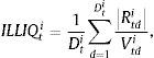
We obtain the aggregate Amihud ratio for the US stock market by taking the cross-sectional average of individual Amihud ratios for each month.11 Finally, we estimate the aggregate measure of illiquidity (ILS) for the US stock market by taking the AR(2) residuals of the regression of the aggregate ratio on its first two lags, as suggested by Acharya and Pedersen (2005).
In addition to aggregate illiquidity measures, we also consider a series of additional aggregate potential determinants of CDS spreads. Corporate CDS spreads might include a premium for bearing risk associated with the state of the economy. To the extent that macroeconomic conditions affect the risk preferences of participants in the CDS market, we would expect to find economic and statistically significant relationships between the CDS spreads and the aggregate variables. To capture the state of the economy or, even more importantly, predict future real activity, we should employ state variables with proven predicting capacity of future output growth.
The term spread, measured as the difference between the interest rates on long- and short-term government debt maturities, is the most common financial leading indicator of real activity. Among others, Estrella and Hardouvelis (1991), Estrella and Mishkin (1998), Stock and Watson (2003), and Ang et al. (2006) identify the significant predictive content of the spread for production growth, including its capacity to forecast a recession indicator in probit regressions. In addition, there is a growing body of literature exploring the transmission of credit conditions into the real economy. Mueller (2009) and Gilchrist et al. (2009) demonstrate the forecasting power of the term structure of credit spreads for future output growth. They argue that there is a pure credit component (orthogonal to macroeconomic conditions) that accounts for a large portion of the predicting capacity of credit spreads. We approximate the slope of the US term structure in interest rates through the difference between 10-year constant maturity Treasury bond yields and the 3-month constant maturity Treasury bill yields (TERM).
To capture the credit conditions, we use the difference between the corporate bond index yields of Bank of America Merrill Lynch (BofA ML) and the Treasury bond yields. We specifically calculate the default spreads for the rating groups of AAA to A−, BBB+ to BBB−, BB+ to BB−, and B+ to D for maturities of 1, 3, 5, 7, and 10 years. For instance, to calculate the default spread of AAA to A− rated bonds with a 10-year maturity (DEF AAA to A10y), we take the difference between the corporate bond index yields of AAA to A− rated bonds and the 10-year constant maturity Treasury bond yields. In further analysis, we also use default spreads by maturity. To calculate the default spread DEF(M)y for a M year maturity, we use the difference between the corporate and Treasury bond yields with M year maturity, respectively. Finally, we calculate the difference between the corporate bond index yields for the investment grade and high yield bonds (DEF) to capture the credit conditions within the IG and HY markets. We download the data on the corporate bond yields of BofA ML from the website of the Federal Reserve Bank of St. Louis.
There has been considerable attention given recently to the role of financial uncertainty as a predictor of real activity. An increasingly popular measure of the risk premium potentially embedded in financial uncertainty is given by the variance risk premium (VRP) (Bollerslev et al., 2009; Longstaff et al., 2011; Zhou, 2010). It is well known that the difference between the realized volatility during a particular month and the risk-neutral counterpart represented by VIX provides the (annualized) monthly volatility risk premium proxy. The realized variance is estimated as the (annualized) squared daily returns for a given month of the S&P500 index. The variance risk premium is reported to be negative on average (see Carr and Wu, 2009). It should be noted that the difference between the realized variance and (the square of) the VIX can be understood as the payoff of a variance swap contract. The average negative payoff of the contract suggests that investors are willing to accept negative returns for purchasing realized variance. Conversely, investors who are sellers of variance and are providing insurance to the market require substantial positive returns. This requirement may be rational because the correlation between volatility shocks and market returns is known to be strongly negative, and investors may desire protection against stock market crashes.
Finally, the aggregate risk preferences of the market participants are proxied by the time-varying relative risk aversion (RA) measure under habit preferences based on the consumption surplus ratio of Campbell and Cochrane (1999). This is estimated as
where St is the surplus consumption ratio given by St=(Ct−Xt)/Ct, Ct is the monthly seasonally adjusted real per capita consumption expenditures on nondurable goods and services, Xt is the level of habit approximated by an autoregressive process consistent with a sufficiently low volatile interest rate, and γ is the inverse of the elasticity of the inter-temporal substitution.122.3Descriptive statistics of aggregate variables
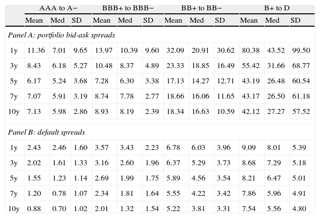
Table 3 provides the summary statistics of the aggregate illiquidity measures and the macroeconomic control variables. In Panels A and B, we further delineate the summary statistics of the aggregate illiquidity measure for the CDS market (given by the aggregate absolute bid-ask spread) and the default spread by portfolio rating and maturity. Panel A shows that for a given credit rating, the shortest maturities are always more illiquid than the longest, which is particularly true for CDS contracts with 1-year maturity. The 5-year CDS contracts are the most liquid, with the exception of the high-yield portfolios, where the 5-, 7-, and 10-year maturities have approximately the same illiquidity level. Therefore, the (average) slope in the term structure of the bid-ask illiquidity for CDS spreads presents an asymmetric U-shaped pattern. At the same time, the standard deviation of portfolio illiquidity decreases almost everywhere as the maturity increases. However, for a given maturity, the portfolio illiquidity increases as the credit quality of the portfolio diminishes. This holds true in portfolio CDS spreads for all maturities in terms of both mean and median, and also holds true for the standard deviation of illiquidity. Moreover, when the maturity is constant, the increase in portfolio illiquidity is considerable when moving from investment grade to high-yield CDS portfolios. For instance, the average of the most liquid 5-year bid-ask spread of AAA/A− and BBB+/BBB− portfolios are approximately 6 and 7 basis points, while the average 5-year bid-ask spread of BB+/B− and B+/D portfolios are approximately 17 and 43 basis points, respectively.
Liquidity proxies and macro variables.
| AAA to A− | BBB+ to BBB− | BB+ to BB− | B+ to D | |||||||||
| Mean | Med | SD | Mean | Med | SD | Mean | Med | SD | Mean | Med | SD | |
| Panel A: portfolio bid-ask spreads | ||||||||||||
| 1y | 11.36 | 7.01 | 9.65 | 13.97 | 10.39 | 9.60 | 32.09 | 20.91 | 30.62 | 80.38 | 43.52 | 99.50 |
| 3y | 8.43 | 6.18 | 5.27 | 10.48 | 8.37 | 4.89 | 23.33 | 18.85 | 16.49 | 55.42 | 31.66 | 68.77 |
| 5y | 6.17 | 5.24 | 3.68 | 7.28 | 6.30 | 3.38 | 17.13 | 14.27 | 12.71 | 43.19 | 26.48 | 60.54 |
| 7y | 7.07 | 5.91 | 3.19 | 8.74 | 7.78 | 2.77 | 18.66 | 16.06 | 11.65 | 43.17 | 26.50 | 61.18 |
| 10y | 7.13 | 5.98 | 2.86 | 8.93 | 8.19 | 2.39 | 18.34 | 16.63 | 10.59 | 42.12 | 27.27 | 57.52 |
| Panel B: default spreads | ||||||||||||
| 1y | 2.43 | 2.46 | 1.60 | 3.57 | 3.43 | 2.23 | 6.78 | 6.03 | 3.96 | 9.09 | 8.01 | 5.39 |
| 3y | 2.02 | 1.61 | 1.33 | 3.16 | 2.60 | 1.96 | 6.37 | 5.29 | 3.73 | 8.68 | 7.29 | 5.18 |
| 5y | 1.55 | 1.23 | 1.14 | 2.69 | 1.99 | 1.75 | 5.89 | 4.56 | 3.54 | 8.21 | 6.47 | 5.01 |
| 7y | 1.20 | 0.78 | 1.07 | 2.34 | 1.81 | 1.64 | 5.55 | 4.22 | 3.42 | 7.86 | 5.96 | 4.91 |
| 10y | 0.88 | 0.70 | 1.02 | 2.01 | 1.32 | 1.54 | 5.22 | 3.81 | 3.31 | 7.54 | 5.56 | 4.80 |
| Mean | SD | Min | 5 | Med | 95 | Max | Obs. | |
| Panel C: aggregate illiquidity proxies and macro variables | ||||||||
| ILBAS1y | 30.20 | 33.32 | 7.86 | 8.63 | 14.83 | 106.41 | 184.66 | 81 |
| ILBAS3y | 20.85 | 19.81 | 6.94 | 8.14 | 12.07 | 54.21 | 143.56 | 81 |
| ILBAS5y | 15.27 | 16.08 | 4.83 | 5.88 | 9.18 | 39.62 | 121.12 | 81 |
| ILBAS7y | 16.32 | 15.42 | 6.54 | 7.57 | 10.68 | 36.19 | 120.43 | 81 |
| ILBAS10y | 16.07 | 14.21 | 6.93 | 7.69 | 11.04 | 32.77 | 113.23 | 81 |
| ILS | −0.03 | 0.46 | −1.92 | −0.46 | −0.04 | 0.49 | 2.52 | 84 |
| RA | 51.13 | 38.11 | 23.74 | 24.26 | 28.58 | 130.24 | 139.00 | 84 |
| VRP | −3.69 | 4.54 | −12.65 | −11.20 | −3.60 | 3.41 | 16.65 | 88 |
| TERM | 1.82 | 1.37 | −0.61 | −0.32 | 2.14 | 3.52 | 3.78 | 88 |
| DEF1y | 1.99 | 1.94 | 0.22 | 0.32 | 1.29 | 7.25 | 7.81 | 88 |
| DEF3y | 2.01 | 1.54 | 0.64 | 0.69 | 1.46 | 5.82 | 6.87 | 88 |
| DEF5y | 2.15 | 1.53 | 0.82 | 0.87 | 1.53 | 6.07 | 6.78 | 88 |
| DEF7y | 2.14 | 1.44 | 0.93 | 0.99 | 1.77 | 5.83 | 6.82 | 88 |
| DEF10y | 2.09 | 1.15 | 1.08 | 1.16 | 1.60 | 5.01 | 5.83 | 88 |
| DEF HYIG | 4.01 | 2.38 | 1.50 | 1.89 | 3.13 | 10.55 | 13.13 | 88 |
This table reports the summary statistics for our illiquidity measures and macroeconomic variables. Panels A and B provide the summary statistics for the bid-ask spread measure of illiquidity of the CDS market and the default spread in terms of maturity and credit quality, respectively. Credit-quality-sorted bid-ask spreads are calculated in the same way as the portfolio CDS spreads, whereas default spreads are calculated by taking the difference between the corporate bond index yields for different rating groups and the Treasury bond yields for different maturities. Panel C provides the summary statistics for the aggregate measures and macroeconomic variables without taking into account the credit quality dimension. ILS is the aggregate measures of illiquidity for US stock market. RA is the time-varying risk aversion under habit preferences based on the consumption surplus ratio. VRP is the variance risk premium, TERM is the term spread of interest rate curve. DEF(M)y is the default spread with M year maturity, and DEF is the difference between corporate bond index yields of HY and IG bonds. The frequency of all measures is monthly. The data for most of the measures are from January 2004 to April 2011, except for the bid-ask spreads and the bond market illiquidity, which end in December 2009 and September 2010, respectively.
Fig. 3 depicts the time series of aggregate bid-ask spreads by maturity. We generally observe that the lower the maturity, the higher the illiquidity of the CDS contracts. This effect is particularly true during stress periods, with the exception being the 5-year contract, which is the most liquid contract overall. As expected, the illiquidity of the CDS market increases substantially after the beginning of the financial crisis and reaches its peak at the end of 2008 – corresponding to the collapse of Lehman Brothers.

Time series of aggregate absolute CDS bid-ask spread. This graph depicts the time series of aggregate bid-ask spreads by maturity. The time series of aggregate bid-ask spreads are obtained by taking the cross-sectional average of individual bid-ask spreads of CDS names in our database for each month and maturity. The time period of our sample extends from January 2004 to September 2010.
Panel B of Table 3 shows that the default spread increases as credit quality decreases, but the spread decreases as the maturity increases. We recall that the default spreads for a given rating group with different maturities are calculated by taking the difference between the corporate bond index yield for that given rating group and the Treasury bond yields at different maturities. Therefore, the decreasing effect of maturity is due to the manner in which the default spreads are defined.
Panel C of Table 3 also reports descriptive statistics for the aggregate illiquidity for alternative horizons without distinguishing across credit quality for bid-ask spreads and default spreads, market-wide illiquidity of the stock market, time-varying risk aversion, the variance risk premium, the slope of the term structure and the default risk between the HY and IG markets, respectively. As previously noted, the aggregate illiquidity measured by the absolute bid-ask spread shows that short-term maturity contracts are highly illiquid, the average variance risk premium is negative, and, on average, the slope and default state variables are positive during our sample period, as expected. Fig. 4 depicts the time series of the aggregate Amihud ratio, the aggregate Amihud illiquidity, and the AR(2) residuals for the US stock market. This series reveals a substantial increase in the aggregate illiquidity of the stock markets when Lehman Brothers went bankrupt. Fig. 5 displays the aggregate time-varying risk aversion under habit preferences. Risk aversion tends to increase during stress periods; however, it is striking to see the enormous increase of risk aversion during the current economic and financial crisis. This figure shows unknown levels of risk aversion, strongly impacting discount rates and financial prices. Fig. 6 represents the annualized volatility risk premium. As expected, the volatility under the risk-neutral measure tends to be higher than the volatility under the objective probability measure, except in periods of great distress, when the realized volatility is extremely high.
 residual of the aggregate Amihud ratio). The time period extends from January 2000 to December 2011.")

. We calculate the VRP by taking the difference between the monthly and realized volatility of the returns of the S&P 500 index (annualized volatility) and the end-of-month value of the VIX index for the corresponding month. The time series extends from January 2000 to January 2012.")
Time series of variance risk premium. This graph depicts the time series of the variance risk premium (VRP). We calculate the VRP by taking the difference between the monthly and realized volatility of the returns of the S&P 500 index (annualized volatility) and the end-of-month value of the VIX index for the corresponding month. The time series extends from January 2000 to January 2012.
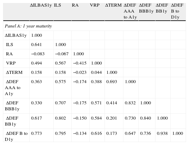
Table 4 displays the correlation matrix among the aggregate illiquidity and other control variables for the entire sample period from January 2004 to September 2010. Though not present in the table, we note that there is a high level of correlation among the bid-ask spreads of CDS contracts for different maturities. Specifically, all the pairwise correlation coefficients between any two series of bid-ask spreads with different maturities are higher than 90%. This suggests that there might be a high commonality in the bid-ask spreads of different maturities.
Correlation matrix of liquidity proxies and macro variables.
| ΔILBAS1y | ILS | RA | VRP | ΔTERM | ΔDEF AAA to A1y | ΔDEF BBB1y | ΔDEF BB1y | ΔDEF B to D1y | |
| Panel A: 1 year maturity | |||||||||
| ΔILBAS1y | 1.000 | ||||||||
| ILS | 0.641 | 1.000 | |||||||
| RA | −0.083 | −0.067 | 1.000 | ||||||
| VRP | 0.494 | 0.567 | −0.415 | 1.000 | |||||
| ΔTERM | 0.158 | 0.158 | −0.023 | 0.044 | 1.000 | ||||
| ΔDEF AAA to A1y | 0.363 | 0.575 | −0.174 | 0.388 | 0.693 | 1.000 | |||
| ΔDEF BBB1y | 0.330 | 0.707 | −0.175 | 0.571 | 0.414 | 0.832 | 1.000 | ||
| ΔDEF BB1y | 0.617 | 0.802 | −0.150 | 0.584 | 0.201 | 0.730 | 0.840 | 1.000 | |
| ΔDEF B to D1y | 0.773 | 0.795 | −0.134 | 0.616 | 0.173 | 0.647 | 0.736 | 0.938 | 1.000 |
| ΔILBAS3y | ILS | RA | VRP | ΔTERM | ΔDEF AAA to A3y | ΔDEF BBB3y | ΔDEF BB3y | ΔDEF B to D3y | |
| Panel B: 3 year maturity | |||||||||
| ΔILBAS3y | 1.000 | ||||||||
| ILS | 0.525 | 1.000 | |||||||
| RA | −0.052 | −0.067 | 1.000 | ||||||
| VRP | 0.412 | 0.567 | −0.415 | 1.000 | |||||
| ΔTERM | 0.159 | 0.158 | −0.023 | 0.044 | 1.000 | ||||
| ΔDEF AAA to A3y | 0.400 | 0.692 | −0.153 | 0.402 | 0.371 | 1.000 | |||
| ΔDEF BBB3y | 0.289 | 0.766 | −0.154 | 0.564 | 0.169 | 0.844 | 1.000 | ||
| ΔDEF BB3y | 0.569 | 0.801 | −0.135 | 0.562 | 0.085 | 0.836 | 0.887 | 1.000 | |
| ΔDEF B to D3y | 0.701 | 0.797 | −0.126 | 0.602 | 0.100 | 0.759 | 0.792 | 0.940 | 1.000 |
| ΔILBAS5y | ILS | RA | VRP | ΔTERM | ΔDEF AAA to A5y | ΔDEF BBB5y | ΔDEF BB5y | ΔDEF B to D5y | |
| Panel C: 5 year maturity | |||||||||
| ΔILBAS5y | 1.000 | ||||||||
| ILS | 0.514 | 1.000 | |||||||
| RA | −0.047 | −0.067 | 1.000 | ||||||
| VRP | 0.367 | 0.567 | −0.415 | 1.000 | |||||
| ΔTERM | 0.212 | 0.158 | −0.023 | 0.044 | 1.000 | ||||
| ΔDEF AAA to A5y | 0.490 | 0.724 | −0.166 | 0.455 | 0.222 | 1.000 | |||
| ΔDEF BBB5y | 0.327 | 0.778 | −0.160 | 0.600 | 0.052 | 0.828 | 1.000 | ||
| ΔDEF BB5y | 0.595 | 0.800 | −0.136 | 0.572 | 0.031 | 0.857 | 0.890 | 1.000 | |
| ΔDEF B to D5y | 0.701 | 0.791 | −0.126 | 0.606 | 0.065 | 0.806 | 0.810 | 0.943 | 1.000 |
| ΔILBAS7y | ILS | RA | VRP | ΔTERM | ΔDEF AAA to A7y | ΔDEF BBB7y | ΔDEF BB7y | ΔDEF B to D7y | |
| Panel D: 7 year maturity | |||||||||
| ΔILBAS7y | 1.000 | ||||||||
| ILS | 0.515 | 1.000 | |||||||
| RA | −0.036 | −0.067 | 1.000 | ||||||
| VRP | 0.363 | 0.567 | −0.415 | 1.000 | |||||
| ΔTERM | 0.211 | 0.158 | −0.023 | 0.044 | 1.000 | ||||
| ΔDEF AAA to A7y | 0.485 | 0.642 | −0.191 | 0.537 | 0.062 | 1.000 | |||
| ΔDEF BBB7y | 0.296 | 0.721 | −0.174 | 0.654 | −0.057 | 0.817 | 1.000 | ||
| ΔDEF BB7y | 0.571 | 0.775 | −0.142 | 0.594 | −0.016 | 0.858 | 0.888 | 1.000 | |
| ΔDEF B to D7y | 0.693 | 0.777 | −0.129 | 0.621 | 0.036 | 0.796 | 0.799 | 0.940 | 1.000 |
| ΔILBAS10y | ILS | RA | VRP | ΔTERM | ΔDEF AAA to A10y | ΔDEF BBB10y | ΔDEF BB10y | ΔDEF B to D10y | |
| Panel E: 10 year maturity | |||||||||
| ΔILBAS10y | 1.000 | ||||||||
| ILS | 0.503 | 1.000 | |||||||
| RA | −0.031 | −0.067 | 1.000 | ||||||
| VRP | 0.348 | 0.567 | −0.415 | 1.000 | |||||
| ΔTERM | 0.217 | 0.158 | −0.023 | 0.044 | 1.000 | ||||
| ΔDEF AAA to A10y | 0.418 | 0.656 | −0.218 | 0.479 | 0.061 | 1.000 | |||
| ΔDEF BBB10y | 0.237 | 0.726 | −0.189 | 0.615 | −0.062 | 0.807 | 1.000 | ||
| ΔDEF BB10y | 0.548 | 0.782 | −0.149 | 0.581 | −0.018 | 0.843 | 0.875 | 1.000 | |
| ΔDEF B to D10y | 0.678 | 0.781 | −0.133 | 0.613 | 0.035 | 0.778 | 0.783 | 0.939 | 1.000 |
This table reports the correlation matrix among aggregate illiquidity variables with different maturities and macro finance variables. The correlation matrix at each maturity is based on the months for which the data on all variables overlap.
The aggregate illiquidity measure for the US equity market has a relatively high (above 0.50 and less than 0.65) correlation with the aggregate illiquidity measures of the CDS spreads. We also observe moderate and positive correlation coefficients between the aggregate illiquidity variable of the CDS market and both the variance risk premium and the changes in default risk. In particular, as the credit quality of a CDS portfolio decreases, the correlation between changes in the bid-ask spreads and changes in the default risk increases across all maturities, with the exception of BBB portfolios. This fact suggests that the aggregate CDS bid-ask spreads might also include a default component, in addition to liquidity. It is interesting to note the negative correlation between the variance risk premium and the aggregate risk aversion. When risk aversion increases, the expected variance under the risk-neutral measure becomes higher relative to realized variance, generating a negative association between these two variables.
3Effects of market-wide illiquidity and default on CDS spreadsWe next investigate the relationship between changes in the CDS spreads and both market-wide illiquidity and default. For a given maturity, and for each portfolio p of a particular credit quality, we run the following OLS autocorrelation-robust standard error regressions:
where ΔCDSpt is the change of the monthly CDS spread of portfolio p for a given maturity, and resILBASyt is the residual that we obtain when regressing changes in an aggregate (equally weighted) absolute bid-ask spread for a given maturity on changes in the default spread for the same maturity; the other variables have been previously defined. We consider the residual measure of the bid-ask spreads as an aggregate measure of illiquidity for the CDS market because, as previously noted, the aggregate CDS bid-ask spreads might include a credit risk component in addition to liquidity. To illustrate this point, consider a CDS contract with party B (protection buyer) buying protection from party S (protection seller) on the credit risk of a reference entity X. At least three situations might arise that will induce either of the parties to suffer losses. First, if the reference entity X underlying the CDS contract defaults, protection seller S might suffer a large unexpected loss and be driven into default. In this scenario, the protection buyer B might not receive the protection payment from the protection seller. Second, protection buyer B can also suffer losses if the protection seller S defaults, even if the reference entity X does not. If this occurs, the protection buyer can terminate the existing contact with the protection seller and buy credit protection on the same entity from a counterparty. However, if the credit quality of the reference entity has decreased, then the new default premium will be higher. This will expose the protection buyer to mark- to-market movements in the default premium. Third, protection seller S can suffer losses if protection buyer B fails to pay the premium for whatever reason. In this scenario, the protection seller S can terminate the existing contract and try to sell protection on the same credit to a counterparty. However, the protection seller will now be exposed to mark-to-market risk. In a world with higher credit risk, the bid-ask spread can not only widen because of the risk of the underlying CDS name X defaulting but also because of the risk of the protection buyer or seller defaulting. Thus, CDS bid-ask spreads can also capture credit risk in addition to illiquidity.
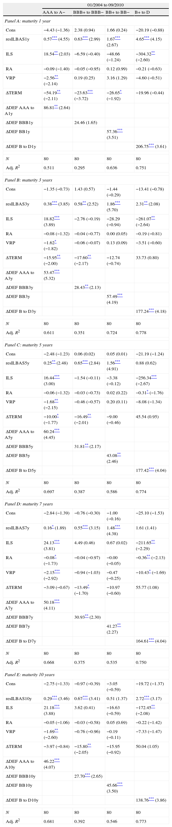
Table 5 contains the regression results for the time period from January 2004 to September 2010, where each panel corresponds to a given horizon of 1-, 3-, 5-, 7-, and 10-year maturities. The key result of this section is the positive relationship between the changes in portfolio CDS spreads and the changes in the aggregate bid-ask spread measure of illiquidity of the CDS market. The regression coefficients, which we interpret as illiquidity CDS betas, are estimated with precision across all credit ratings and maturities. In many of the specifications of the portfolio CDS maturity and rating groups, the illiquidity betas are positive and statistically significant for standard confidence levels. Moreover, as one would expect, the magnitude of the coefficients tends to be larger for high yield underlyings. Therefore, the low credit rating CDS spreads tend to be highly sensitive to aggregate illiquidity shocks relative to the high credit quality CDS spreads. This suggests that changes of the CDS spreads are determined by more than the changes in the credit quality of the underlying corporate bond.
Portfolio CDS spreads, aggregate CDS bid-ask spread and stock illiquidity.
| 01/2004 to 09/2010 | ||||
| AAA to A− | BBB+ to BBB− | BB+ to BB− | B+ to D | |
| Panel A: maturity 1 year | ||||
| Cons | −4.43 (−1.36) | 2.38 (0.94) | 1.66 (0.24) | −20.19 (−0.88) |
| resILBAS1y | 0.57*** (4.55) | 0.63*** (2.99) | 1.67*** (2.67) | 4.65*** (4.15) |
| ILS | 18.54** (2.03) | −6.59 (−0.40) | −48.66 (−1.24) | −304.32** (−2.60) |
| RA | −0.09 (−1.40) | −0.05 (−0.95) | 0.12 (0.99) | −0.21 (−0.63) |
| VRP | −2.56** (−2.14) | 0.19 (0.25) | 3.16 (1.29) | −4.60 (−0.51) |
| ΔTERM | −54.19** (−2.11) | −23.63*** (−3.72) | −26.65* (−1.92) | −19.96 (−0.44) |
| ΔDEF AAA to A1y | 86.81** (2.64) | |||
| ΔDEF BBB1y | 24.46 (1.65) | |||
| ΔDEF BB1y | 57.36*** (3.51) | |||
| ΔDEF B to D1y | 206.75*** (3.61) | |||
| N | 80 | 80 | 80 | 80 |
| Adj. R2 | 0.511 | 0.295 | 0.636 | 0.751 |
| Panel B: maturity 3 years | ||||
| Cons | −1.35 (−0.73) | 1.43 (0.57) | −1.44 (−0.29) | −13.41 (−0.78) |
| resILBAS3y | 0.38*** (3.85) | 0.58** (2.52) | 1.86*** (5.70) | 2.31** (2.08) |
| ILS | 18.82*** (3.89) | −2.76 (−0.19) | −28.29 (−0.94) | −261.07** (−2.64) |
| RA | −0.08 (−1.32) | −0.04 (−0.77) | 0.00 (0.05) | −0.19 (−0.81) |
| VRP | −1.62* (−1.82) | −0.06 (−0.07) | 0.13 (0.09) | −3.51 (−0.60) |
| ΔTERM | −15.95** (−2.00) | −17.60** (−2.17) | −12.74 (−0.74) | 33.73 (0.80) |
| ΔDEF AAA to A3y | 53.47*** (5.32) | |||
| ΔDEF BBB3y | 28.43** (2.13) | |||
| ΔDEF BB3y | 57.49*** (4.19) | |||
| ΔDEF B to D3y | 177.24*** (4.18) | |||
| N | 80 | 80 | 80 | 80 |
| Adj. R2 | 0.611 | 0.351 | 0.724 | 0.778 |
| Panel C: maturity 5 years | ||||
| Cons | −2.48 (−1.23) | 0.06 (0.02) | 0.05 (0.01) | −21.19 (−1.24) |
| resILBAS5y | 0.25** (2.48) | 0.65*** (2.84) | 1.56*** (4.91) | 0.88 (0.62) |
| ILS | 16.44*** (3.00) | −1.54 (−0.11) | −3.38 (−0.12) | −256.34*** (−2.67) |
| RA | −0.06 (−1.32) | −0.03 (−0.73) | 0.02 (0.22) | −0.31* (−1.76) |
| VRP | −1.68** (−2.15) | −0.46 (−0.57) | 0.20 (0.11) | −8.08 (−1.34) |
| ΔTERM | −10.00* (−1.77) | −16.49** (−2.01) | −9.00 (−0.46) | 45.54 (0.95) |
| ΔDEF AAA to A5y | 60.24*** (4.45) | |||
| ΔDEF BBB5y | 31.81** (2.17) | |||
| ΔDEF BB5y | 43.08** (2.46) | |||
| ΔDEF B to D5y | 177.42*** (4.04) | |||
| N | 80 | 80 | 80 | 80 |
| Adj. R2 | 0.697 | 0.387 | 0.586 | 0.774 |
| Panel D: maturity 7 years | ||||
| Cons | −2.84 (−1.39) | −0.76 (−0.30) | −1.00 (−0.16) | −25.10 (−1.53) |
| resILBAS7y | 0.16* (1.89) | 0.55*** (3.15) | 1.48*** (4.38) | 1.61 (1.41) |
| ILS | 24.13*** (3.81) | 4.49 (0.46) | 0.67 (0.02) | −211.65** (−2.29) |
| RA | −0.08* (−1.73) | −0.04 (−0.97) | −0.00 (−0.05) | −0.36** (−2.13) |
| VRP | −2.15*** (−2.92) | −0.94 (−1.03) | −0.47 (−0.25) | −10.43* (−1.69) |
| ΔTERM | −3.09 (−0.67) | −13.49* (−1.70) | −10.97 (−0.60) | 55.77 (1.08) |
| ΔDEF AAA to A7y | 50.18*** (4.11) | |||
| ΔDEF BBB7y | 30.93** (2.30) | |||
| ΔDEF BB7y | 41.27** (2.27) | |||
| ΔDEF B to D7y | 164.61*** (4.04) | |||
| N | 80 | 80 | 80 | 80 |
| Adj. R2 | 0.668 | 0.375 | 0.535 | 0.750 |
| Panel E: maturity 10 years | ||||
| Cons | −2.75 (−1.33) | −0.97 (−0.39) | −3.05 (−0.59) | −19.72 (−1.37) |
| resILBAS10y | 0.29*** (3.46) | 0.67*** (3.41) | 0.51 (1.37) | 2.72*** (3.17) |
| ILS | 21.18*** (3.88) | 3.62 (0.41) | −16.63 (−0.59) | −172.45** (−2.08) |
| RA | −0.05 (−1.06) | −0.03 (−0.58) | 0.05 (0.69) | −0.22 (−1.42) |
| VRP | −1.69** (−2.60) | −0.76 (−0.96) | −0.19 (−0.11) | −7.33 (−1.47) |
| ΔTERM | −3.97 (−0.84) | −15.80** (−2.05) | −15.95 (−0.92) | 50.04 (1.05) |
| ΔDEF AAA to A10y | 46.22*** (4.07) | |||
| ΔDEF BBB10y | 27.70*** (2.65) | |||
| ΔDEF BB10y | 45.66*** (3.50) | |||
| ΔDEF B to D10y | 138.76*** (3.86) | |||
| N | 80 | 80 | 80 | 80 |
| Adj. R2 | 0.681 | 0.392 | 0.546 | 0.773 |
This table reports monthly regressions with changes in portfolio CDS spread (equally weighted) with different maturities as a dependent variable. t-Statistics are calculated based on standard errors corrected for autocorrelation and heteroscedasticity (Newey–West). N denotes the number of observations used in the regression analysis. Adj. R2 denotes the adjusted R2 statistics. resILBAS(M)y denotes residuals that we obtain when regressing changes in the aggregate CDS bid-ask spread with M year maturity on changes of Default spread with M year maturity. ILS is the aggregate measures of illiquidity for the US stock market. RA denotes the time-varying risk aversion under habit preferences based on the consumption surplus ratio. VRP denotes the level of variance risk premium. ΔTERM denotes changes in term spread, and ΔDEF(P)(M)y denotes the changes in default spreads for credit portfolio P with M year maturity.
t statistics in parentheses.
The aggregate measure of Amihud illiquidity of the US equity market tends to be a significant factor for AAA to A− and B+ to D rated CDS portfolios. The regression coefficients are positive for AAA to A− rated CDS portfolios and negative for B+ to D portfolios, and both groups are estimated with precision. Therefore, the possible spillover effects of market-wide illiquidity equity shocks seem to be particularly relevant for the highest and lowest rated underlyings, respectively. However, the negative coefficients for the B+ to D credit portfolios are puzzling.
The uncertainty embedded in financial assets and proxied by the volatility risk premium is primarily related to the AAA to A- CDS portfolios. The regression coefficients of these CDS portfolios are negatively and significantly related to the VRP. Therefore, it seems that equity volatility shocks only impact the CDS spreads of highly rated underlyings. It is interesting to note the negative relationship between the VRP and the CDS spreads. It should be recalled that the VRP is estimated as the difference between the ex post realized volatility and the VIX. This is the payoff of the future contract on realized variance; when the realized volatility is not as high as expected, traders on the CDS market interpret the lower observed volatility as good news for the economy, and the CDS spreads become lower.
Time-varying risk aversion under habit preferences does not seem to consistently affect price in the CDS spread market. Most of the coefficients are insignificant or estimated with very low precision.
In general, inverted zero-coupon curves tend to anticipate recessions, while upward-sloping curves tend to forecast expansions. This suggests that increases in TERM should be negatively related to changes in CDS spreads. This state variable does not seem to be a consistently important factor in the CDS market. The regression coefficients tend to be negative, but they are estimated with very low precision. The exception is the behavior of BBB+ to BBB− credit quality portfolios (which show relatively precise coefficients) and AAA to A− credit portfolios (especially at short horizons). It may be that these segments are dominated by an industry particularly sensitive to interest rate risks.
Finally, changes in the default spread DEFpt for different credit ratings p and maturities t are one of the key factors that consistently explain changes in CDS spreads. DEFpt reflects the aggregate default risk, and we therefore expect a positive sign for the regression coefficients (this is generally the case). Moreover, the lower the credit quality of the portfolios, the stronger the positive relationship between the default risk and the CDS spreads, with the exception of AAA to A− CDS portfolios. For nearly all credit portfolios, the regression coefficients for the default spread become lower with a longer maturity of the CDS contract.
Overall, our selected market-wide variables explain a high percentage of the variability of the CDS portfolios, except for the BBB+ to BBB− rated CDS portfolio. On average, the R-squared statistics for all portfolios (except for BBB+ to BBB−) is approximately 0.67 for the sample period across all five maturities, and 0.36 for the BBB+ to BBB- CDS portfolio. Overall, the model best fits the lowest rated CDS portfolio.13
To sum up, market-wide illiquidity in the CDS market and default risk are the aggregate variables that are systematically related to changes in CDS spreads. In addition, financial uncertainty represented by the volatility risk premium is consistently associated with the AAA to A− CDS portfolio.
4ConclusionsThis paper examines empirically the relevance of default and illiquidity of CDS spreads at an aggregate level. Our results suggest that measures of both aggregate default and illiquidity can explain changes in CDS spreads. There is a positive and significant relationship between changes in CDS spreads and changes in both aggregate bid-ask spreads and default for a given maturity of a CDS contract. Even after extracting potentially confounding credit risk exposure from the bid-ask spreads, both illiquidity and default (CDS) betas across credit quality portfolios and maturities are positive and statistically significant. Moreover, as one would expect, the magnitude of the coefficients tends to be larger for high-yield underlyings. Therefore, low credit rating CDS spreads tend to be highly sensitive to aggregate default and illiquidity shocks relative to high credit quality CDS spreads.
In order to explore the relationship between CDS spreads and default and illiquidity at an aggregate level, we construct CDS portfolios sorted by credit quality and maturity. We consider a relatively long time period for our analysis that spans from 2004 to 2011. In addition to aggregate default and illiquidity measures, we include several other aggregate explanatory variables in our regressions, such as term spread, volatility risk premium, risk aversion, and an illiquidity measure for the US stock market. Only the volatility risk premium seems to be systematically related to AAA to A- portfolio of CDS spreads.
In conclusion, our results suggest that changes in aggregate CDS spreads are determined by changes in market-wide illiquidity in addition to aggregate credit risk. Policies oriented toward frictionless functioning of CDS markets can enhance liquidity and credit-trading roles of CDS markets, which in turn can improve the quality of CDS spreads as a measure of creditworthiness of companies.
Some earlier papers have considered CDS as a pure measure of default. For instance, Blanco et al. (2005) find that CDS spreads are a cleaner indicator of credit risk than bond spreads. They also find that CDS prices lead bond markets in the price discovery process. In a similar fashion, Longstaff et al. (2005) extract default and non-default components from bond spreads assuming CDS spreads are a pure measure of default risk.
I am grateful to G. Rubio and P. Serrano for excellent comments and suggestions. I would like to thank for constructive comments of A. Novales, J. van Bommel, A. León, A. Cartea, G. Markarian, J. Penalva and S. Gissler, as well as of other conference participants at the 2012 Foro de Finanzas, 2013 EFMA Annual Meeting, and 2013 Armenian Economic Association Annual Meeting.
See Bao et al. (2011), Lin et al. (2011), and Acharya et al. (2013), among others.
Due to the OTC nature of CDS market, the volume of CDS trades is not available. However, many empirical papers consider CDS contract with 5 year maturity to be the most actively traded, while the evidence for liquidity in CDS contracts with other maturities is mixed.
See Jarrow (2011) for an overall discussion on the CDS market and the website of Federal Reserve of St. Louis for a detailed timeline of the credit events associated with the subprime financial crisis (http://timeline.stlouisfed.org).
Schneider et al. (2009) note that the one-year CDS spread exhibits time-varying behavior that higher-maturity spreads do not share. They presume that investment funds primarily use the one-year CDS spreads to express their views on the creditworthiness of CDS names. Therefore, they argue that the economic driver behind the unique pattern in one-year spreads is a supply-and-demand premium induced by these large traders. It should be noted, however, that the pattern shown in Fig. 1 is the complete and monotonic inversion of the slope of the term structure. This implies that this phenomenon is not uniquely related to the shortest maturity CDS spreads.
Before calculating the portfolio CDS spreads, the 1st and 99th percentiles of the CDS spreads are removed from the cross-sectional distribution of the CDS spreads for each month and maturity.
We remove the 1st and 99th percentiles of the CDS bid-ask spreads from their respective distribution for each month and maturity.
See Bongaerts et al. (2011) and Pires et al. (2010) for a formal argument.
To calculate the aggregate bid-ask spread measure of illiquidity for the CDS market, we use the bid and ask quotes from the CMA database for the companies that coincide with those in the Markit database. We then compare the difference in monthly CDS spreads between these two sources by using the measure of mean absolute error (MAE). The mean (median) of the MAE for the average of the bid and ask quotes from the CMA database and the CDS spreads from the Markit database across all coinciding companies are 37 (14), 25 (7), 19 (3), 21 (5), and 25 (8) basis points for maturities of 1, 3, 5, 7, and 10 years, respectively.
We use data from CRSP and only data on stock returns and trading volume from the NYSE.
Before calculating the aggregate Amihud ratio for the equity market, we remove the stock returns that fall outside the 1st and 99th percentile of the cross-sectional distribution of stock returns per trading volume (Rtdi/Vtdi) for each day.
We obtain nominal consumption expenditures on nondurable goods and services from Table 2.8.5 of the National Institute of Pension Administrators (NIPA). Population data are from NIPA's Table 2.6 and the price deflator is computed by using prices from NIPA's Table 2.8.4, with the year 2000 used as its basis. All this information is used to construct monthly seasonally adjusted real per capita consumption expenditures on nondurable goods and services. The autoregressive parameter of the habit process is estimated using the price-dividend ratio obtained from the original series on Robert Shiller's website. The actual procedure to estimate the surplus consumption ratio follows the methodology described by Campbell and Cochrane (1999) with γ=2.
Alternative specifications with either levels or changes of RA and VRP, and with or without RA or TERM, do not seem to affect the overall conclusions.

