


The modulation of tourism time series was used in this work for forecast purposes. The Tourism Revenue and Total Overnights registered in the hotels of the North region of Portugal were used for the experimented models. Several feed-forward Artificial Neural Networks (ANN) models using different input features and number of hidden nodes were experimented to forecast the Tourism time series. Empirical results indicate that the Dedicated ANN models perform better than models with several outputs. Generally the usage of previous 12 values of the same time series is very important to a good quality forecast. For the prediction of Tourism Revenue the Foreign Overnights and GDP of contributing countries are relevant. This time series was predicted with an error of 4.7% and a Pearson correlation of 0.98. The forecast of Total Overnights had an error of 6.0% and Pearson correlation of 0.98. Domestic Overnights are more predictable than Foreign Overnights.
Tourism has been seen as one of the important drivers of economic growth. As a consequence it has become a vital economic activity for developing countries. The role of this activity to the global and national economies, in terms of national outcomes, employment opportunities, foreign exchange earnings and exports, is noteworthy. According to the World Travel and Tourism Council (WTTC), the direct contribution of Travel and Tourism to Gross Domestic Product (GDP) was USD 2,056 billion (2.9% of total GDP) in 2012, and it is forecast to rise by 3.1% in 2013, and also generate over 260 million jobs in 2012 (WTTC, 2013). Travel and Tourism investment in 2012 was USD 764.7 billion, or 4.7% of total investment and it should rise by 4.2% in 2013, according to recent results from WTTC (2013).
Similar to what has been happening in the world, it has been noted in Portugal. Hence, and according to WTTC (2013), the total contribution of tourism sector to GDP was EUR 26.4 billion (15.9% of GDP) in 2012, and it is forecast to rise by 0.2% in 2013; the total contribution to employment, including jobs indirectly supported by the industry, was 18.5% of total employment (860,500 jobs), in 2012, and it is expected to rise by 1% to 954,000 jobs in 2023; the investment in 2012 was EUR 3.5 billion, or 13.2% of total investment and it should rise by 3.3% in 2013.
In the North Region of Portugal and according to the data produced by Portuguese National Institute of Statistics (INE) in 2011, tourism accommodation activity establishments hosted around 3 million guests, originating 4,547 million overnight stays, INE (2012). According to the same source the average stay on the establishment were approximately 2 nights. The total number of establishment registered were around 453 hotels and boarding houses. The net bed-occupancy rate in 2011 were 32.1% and 3.8 thousand euros lodging income per lodging capacity (INE, 2012).
In this regard and because of the continuing growth of tourism, at the international and national levels, and its importance in the economy of a country, there is a need to analyze and forecast the tourism revenues, tourism demand and other time series related with the tourism sector. Indeed, each country wants to know its international and national tourist behaviour and tourism revenues in order to select a suitable strategy for its economic health.
Hence, considering this important factor several studies have been published in the field of tourism in recent years using different methodologies based on versatile nonlinear models that can represent both nonseasonal and seasonal time series. E.g.: Law and Au (1999), Law (2000), Pai and Hong (2005), Chen and Wang (2007), Fernandes, Teixeira, Ferreira, and Azevedo (2008), Fernandes and Teixeira (2009), Machado, Teixeira, and Fernandes (2010), Hong, Dong, Chen, and Wei (2011), Chen (2011), Shen, Li, and Song (2011), Lin, Chen, and Lee (2011), Chen, Lai, and Yeh (2012), Teixeira and Fernandes (2012), Shahrabi, Hadavandi, and Asadi (2013), Lin, Pai, Lu, and Chang, (2013), Pai, Hung, and Lin (2014), and Claveria and Torra (2014). For example Law and Au (1999) used a feed-forward neural network model to forecast Japanese tourism demand. Law (2000) applied a backpropagation neural network to forecast tourism demand. Pai and Hong (2005) employed support vector machines neural networks with genetic algorithms to forecast the arrival data in Barbados. Chen and Wang (2007) applied support vector regression neural networks with genetic algorithms in forecasting tourism demand. Fernandes et al. (2008) investigated and highlighted the usefulness of the Artificial Neural Networks methodology as an alternative to the Box–Jenkins methodology in analysing tourism demand. Fernandes and Teixeira (2009) developed a new approach of the Artificial Neural Networks methodology using the time in its input instead of the previous 12 registered observations, as usually used; the authors intended to compare the classic usage of the Artificial Neural Networks methodology with a new modulation using the years and month in the input. Machado et al. (2010), performed a comparative study between the models based on the linear regression and based on the methodology of artificial neural networks. Hong et al. (2011) presented a support vector regression with chaotic genetic algorithm to forecast tourism demand. Chen (2011) used support vector regression technology to forecast tourism demand. Shen et al. (2011) developed six combination methods to forecast UK outbound tourism demand in seven destination countries. Lin et al. (2011), tried to build the forecasting model of visitors to Taiwan using three commonly adopted ARIMA, artificial neural networks, and multivariate adaptive regression splines. Chen et al. (2012) developed a new forecasting model based on empirical mode decomposition and neural network to predict tourism demand. Teixeira and Fernandes (2012) applied the traditional feed-forward architecture, the cascade forwards, a recurrent Elman architecture and a radial based architecture to forecast the tourism demand. Shahrabi et al. (2013) proposed a new hybrid intelligent model that is called Modular Genetic-Fuzzy Forecasting System by a combination of genetic fuzzy expert systems and data pre-processing which includes K-means clustering and the Takagi–Sugeno–Kang. Lin et al. (2013), developed a fuzzy least-squares support vector regression model with genetic algorithms to forecast seasonal revenues. Pai et al. (2014) developed a novel forecasting system for accurately forecasting tourism demand where the construction of the new forecasting system combines fuzzy c-means with logarithm least-squares support vector regression technologies.
Claveria and Torra (2014) evaluated the forecasting performance of an artificial neural network approach relative to different tourism time series models, autoregressive integrated moving average models and self-exciting threshold autoregressions. Empirical evidence of the studies presented above shows that nonlinear models that can represent both nonseasonal and seasonal time series generally outperform the linear methods in modelling tourism behaviour, as classical time series models, such as ARIMA, linear regression model, multivariate adaptive regression splines and multiple regression, exponential smoothing, moving average and naïve.
Therefore, the aim of this paper is to forecast the time series of tourism, namely the Tourism Revenue, Total Overnights, Domestic and Foreign Overnights in establishment registered in the North of Portugal, using the ANN methodology and find the best architecture to achieve it.
In order to answer the objective of this study the rest of the paper is organized as follows: Section 2 briefly describes the times series and data set under study; Section 3 presents the methodological approach; Section 4 presents the empirical results and analysis, while the final section summarizes the conclusions.
2Description of time seriesAll data were collected from Portuguese National Institute of Statistics, EUROSTAT and Statistical Yearbook for the North Region of Portugal. The data corresponds to 72 monthly observations between January 2006 and December 2011.
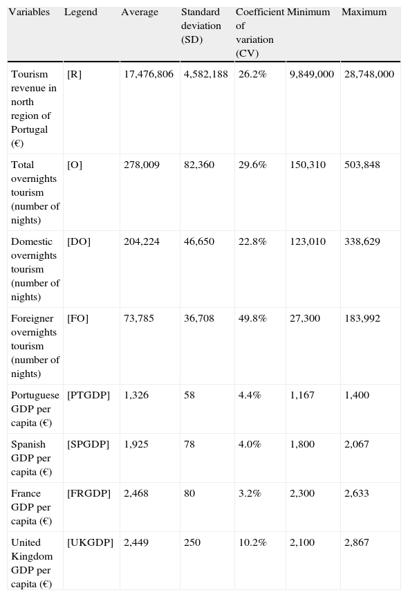
The variables used in this study are symbolized and described in Table 1, accompanied by a descriptive statistics. It should be noted that the selection of GDP for only 4 countries: Portugal, Spain, France and the United Kingdom, were because they are the tourism outbound markets with the main market share for the years under analysis (INE, 2012). The Total Overnights Tourism corresponds to the sum of both Domestic and Foreign’ Overnights.
Descriptive statistics for the variables used in the model.
| Variables | Legend | Average | Standard deviation (SD) | Coefficient of variation (CV) | Minimum | Maximum |
| Tourism revenue in north region of Portugal (€) | [R] | 17,476,806 | 4,582,188 | 26.2% | 9,849,000 | 28,748,000 |
| Total overnights tourism (number of nights) | [O] | 278,009 | 82,360 | 29.6% | 150,310 | 503,848 |
| Domestic overnights tourism (number of nights) | [DO] | 204,224 | 46,650 | 22.8% | 123,010 | 338,629 |
| Foreigner overnights tourism (number of nights) | [FO] | 73,785 | 36,708 | 49.8% | 27,300 | 183,992 |
| Portuguese GDP per capita (€) | [PTGDP] | 1,326 | 58 | 4.4% | 1,167 | 1,400 |
| Spanish GDP per capita (€) | [SPGDP] | 1,925 | 78 | 4.0% | 1,800 | 2,067 |
| France GDP per capita (€) | [FRGDP] | 2,468 | 80 | 3.2% | 2,300 | 2,633 |
| United Kingdom GDP per capita (€) | [UKGDP] | 2,449 | 250 | 10.2% | 2,100 | 2,867 |
For the period under consideration, and analysing information presented in Table 1, it can be seen that Tourism Revenue in the North Region of Portugal was registered as a minimum value of 9,849 thousand € and a maximum value of 28,718 thousand €, corresponding to an average of 17,467 thousand € (Standard Deviation (SD) of 4,582 thousand €), presenting a moderate Coefficient of Variation (CV). With regard to Total Overnights Tourism registered in hotel establishments, a mean of 278,009 overnights (SD 82,360 overnights) was obtained between a minimum of 150,310 overnights and a maximum of 503,848 overnights, having been registered as a high CV consequence of quite high CV verified in the Overnights Foreigner time series (49%). Regarding GDP per capita, it can be observed that the country with the lowest values is Portugal, the highest is France, and the UK showed a higher CV thus showing a greater dispersion of data.
Fig. 1 displays the time series Total Monthly Tourism Revenue in the North Region of Portugal between January 2006 and December 2011. It is possible to observe the increased trend during the period under analysis. This increase was probably affected by the policy of public and private investment undertaken in some facilities and establishments of four and five star categories, because it was a policy established in the Strategic Plan for the North of Portugal. Also, the advertising campaigns for the national and international tourism markets, which were based on suitable and adjusted marketing strategies to the new preferences of tourism consumers, were more likely to appreciate the landscape, nature, gastronomy and cultural heritage. These kinds of factors may contribute to an increased flow of tourists visiting the region.

The Fig. 2 shows total domestic and foreign monthly overnights of tourists in the north region of Portugal. The behaviour of the time series indicates that there is seasonality. An increase from 2006 to 2007 is also evident and corresponds to a positive variation of 9.2%, and then there is a significant decrease in 2008 (negative variation of 1.74%), with a significant growth in 2009 and 2011. The same behaviour was noted for both domestic and foreigner time series. As stated above the trend can be a result of economic growth and investment in the tourism sector, such as in marketing variables that promoted the region both nationally and internationally, which have occurred in northern Portugal in recent years. However, this trend apparently is not linear.

The GDP indicators (Fig. 3) clearly show a slight growth for the time series GDP of Portugal, Spain and France. On the other hand it is possible to observe an abrupt decay for the time series GDP of the United Kingdom.
3Methodology3.1Neural network
A neural network consists of a set of interconnected artificial neurons, structured in layers, nodes, perceptrons or a group of processing units, which process and transmit information through activation functions. The nodes of one layer are connected to the nodes of the next layer to which they can send information. The connections between nodes i and j of previous and following layers are associated with a weight Wij. Each neuron also has a bias bi associated with it. Fig. 4 presents the general architecture used in this work. The activation functions used are the hyperbolic tangent functions in the nodes of the hidden layer and the linear function in the output nodes, Bishop (1995), Haykin (1999), and Rumelhart and McClelland (1986). These architecture connections of the neural network model are known as feed-forward architecture. The neural network can learn based on several input/output pairs. This learning process consists in the adjustment of the weight of the connections between nodes of successive layers and is known as the training process. The most commonly used algorithm to train a feed-forward is the backpropagation algorithm, Rumelhart and McClelland (1986). Several improvements of the original algorithm have been proposed with different performances in different type of applications. In this work the ANNs were trained most of the times using the Levenberg–Marquardt algorithm, Hagan and Menhaj (1994) and Marquardt (1963).

Considering the set of available data and the objectives, several methodologies/Model were experimented with the purpose to predict the Tourism Revenue, and the Total, Domestic and Foreign Tourism Overnights. The Total Tourism Overnights were also predicted by the addiction of the Domestic Overnights and the Foreign Overnights. Several combinations of input features were used for each model. Moreover different number of hidden nodes of the ANN was also experimented.
3.2Training processThe training of the models detailed in the next section were performed with a training data set using a validation set for cross validation to stop training earlier in order to avoid overfitting to the training data set. Another set, the test set, were used to measure the forecast ability of the ANN using never seen data during the training. Hence, the validation sets consisting the 12 values of the months of the year 2010 and the test sets consisting the 12 values of the months of the year 2011. The remaining values were used for training set, consisting of 36 or 48 values (depending on the model) for the years between 2006 and 2007 until 2009.
Once the final weights matrix of the ANN depends on their initial values, 50 training sessions were performed for each model and the best Root Mean Squared Error (RMSE) in the validation set was selected as the weights matrix for this model and used to simulate the output prediction for the test set.
The number of input/output pairs used to train the ANNs is 36 or 48 only. This aspect can be seen as the drawback of this modulation because there are no data enough to adjust conveniently all the weights of the ANN. Therefore the number of nodes in the hidden layer must be kept low in order to have a relatively small number of weights to adjust. Anyhow despite the small number of hidden nodes due to the short training data set the ANN easily goes to an overfitting situation. In these cases the usage of the validation set avoids this situation if the RMSE in the validation set does not improve after 6 successive iterations. The final value of the matrix of weights is the one observed 6 iterations before.
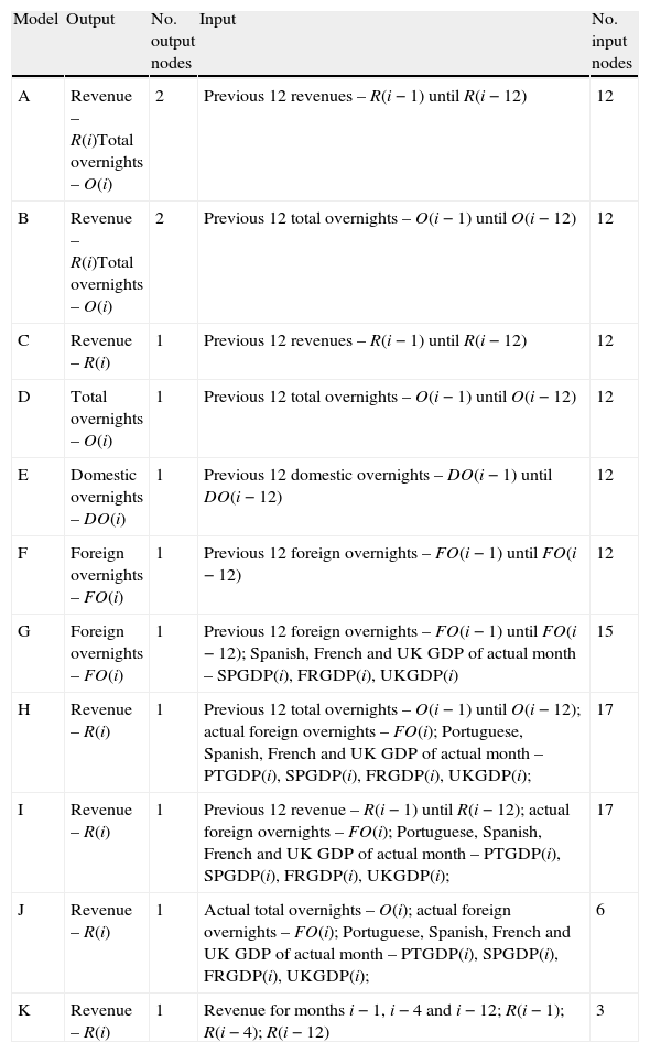
3.3ModelsANN based models were used to predict Tourism Revenue, Total Overnights, Domestic Overnights and Foreign Overnights. Table 2 presents the set of experimented models, its outputs and inputs and number of nodes in the output and input. A total of 11 main models (from A to K) were experimented with different inputs and outputs. Most of the model had 3 variants according to the number of nodes in the hidden layer.
Input and Output of models.
| Model | Output | No. output nodes | Input | No. input nodes |
| A | Revenue – R(i)Total overnights – O(i) | 2 | Previous 12 revenues – R(i−1) until R(i−12) | 12 |
| B | Revenue – R(i)Total overnights – O(i) | 2 | Previous 12 total overnights – O(i−1) until O(i−12) | 12 |
| C | Revenue – R(i) | 1 | Previous 12 revenues – R(i−1) until R(i−12) | 12 |
| D | Total overnights – O(i) | 1 | Previous 12 total overnights – O(i−1) until O(i−12) | 12 |
| E | Domestic overnights – DO(i) | 1 | Previous 12 domestic overnights – DO(i−1) until DO(i−12) | 12 |
| F | Foreign overnights – FO(i) | 1 | Previous 12 foreign overnights – FO(i−1) until FO(i−12) | 12 |
| G | Foreign overnights – FO(i) | 1 | Previous 12 foreign overnights – FO(i−1) until FO(i−12); Spanish, French and UK GDP of actual month – SPGDP(i), FRGDP(i), UKGDP(i) | 15 |
| H | Revenue – R(i) | 1 | Previous 12 total overnights – O(i−1) until O(i−12); actual foreign overnights – FO(i); Portuguese, Spanish, French and UK GDP of actual month – PTGDP(i), SPGDP(i), FRGDP(i), UKGDP(i); | 17 |
| I | Revenue – R(i) | 1 | Previous 12 revenue – R(i−1) until R(i−12); actual foreign overnights – FO(i); Portuguese, Spanish, French and UK GDP of actual month – PTGDP(i), SPGDP(i), FRGDP(i), UKGDP(i); | 17 |
| J | Revenue – R(i) | 1 | Actual total overnights – O(i); actual foreign overnights – FO(i); Portuguese, Spanish, French and UK GDP of actual month – PTGDP(i), SPGDP(i), FRGDP(i), UKGDP(i); | 6 |
| K | Revenue – R(i) | 1 | Revenue for months i−1, i−4 and i−12; R(i−1); R(i−4); R(i−12) | 3 |
Both the revenue and the overnights can reflect the tourism demand. The experimented models intend to predict these time series together in the same model (A and B models) or isolated in different models. Therefore, the Total Overnights is the time series to be predicted in Models A, B and D. Model E predicts Domestic overnights, and models F and G predict Foreign Overnights. The combination of the output of Model E and one of the models F or G gives the Total Overnights. The Revenue time series were predicted by models A, B, C, H, I and J.
Models A and B predicts simultaneously two outputs, Revenue and Total Overnights. For these cases the selection of the best weights matrix during training sessions can be made by the minimization of the RMSE of the validation set of the output Total Overnights and the RMSE of the validation set of the output Revenue.
All models, except model J, use the previous 12 months in the input. Therefore, for these models only 36 months (input/output pairs) were available for training. Model J had 48 input/output training pairs.
For each model 6, 8 and 10 nodes in the hidden layer were experimented, which have been denominated as the sub-models.
4Empirical resultsThe results for the test, validation and the all database (total) sets will be analyzed in this section, comparing the real values observed (target) with the forecast values for each model/sub-model using different number of nodes in the hidden layer. It should be mentioned that the validation set consists of the 12 months of the year 2010 and the test set the 12 months of the year 2011.
The Total set consists of training, validation and test sets together. This Total set gives a perception of how the model behaves in a longer time data set, but these results cannot be taken as the true evaluation of the model because most of the data were used during training process.
The validation set was used to stop the training process early. The error in this set is the best the models achieved during the 50 training sessions with data not directly used to adjust the weights of the ANN. It can be seen as the lower error the model can achieve.
The test set consists only in data never seen during training process and therefore it can be used to evaluate the model with real and true new data. The error in this set can be taken as the more serious one to evaluate the model in a real and new situation.
Although the performance of each model is presented below for the three sets the analysis of the best model will be made regarding only the performance in test set.
The Mean Absolute Percentage Error (MAPE) was used to measure the error distance between the predicted and the target values of the time series, according to following equation.
where N is the length of the set, T and P are the target and predicted values for month i. Lower the MAPE, more close are the predicted data to the target data and therefore better is the prediction model.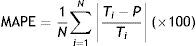
The Pearson correlation coefficient (r) between the target and predicted vectors of the time series is also analyzed. As closer to 1 is the r, more similar are the variation patterns of predicted and target data. Anyhow this parameter is not sensitive to differences between scales of the two sets of values nor even is it sensitive to a constant variation (offset) between sets.
These two parameters (MAPE and r) can give different type of information about the ability of the model to fit the time series data. The MAPE is an indication of how far is the predicted data set of the target data set, meanwhile the Pearson correlation coefficient gives a measure of how different is the curve pattern of the two data sets.
Using a number of nodes lower than 8 the MAPE is very high (experiments not presented in tables).
The usage of more nodes than 12 in the hidden layer increases the number of weights to be adjusted but the number of input/output pairs is not enough.
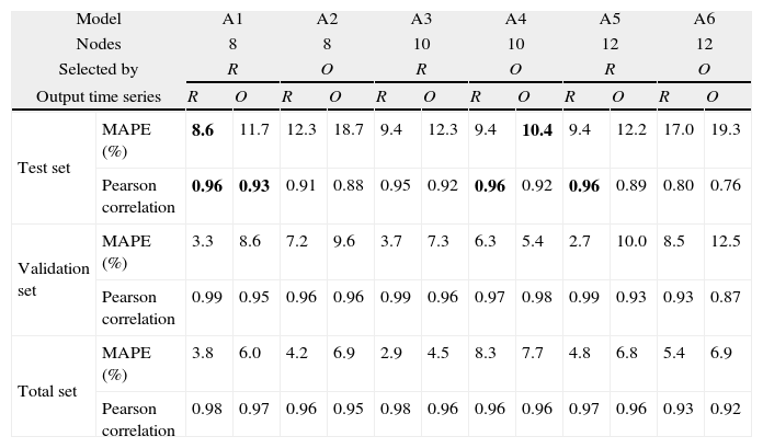
4.1Model ATable 3 presents the MAPE and Pearson correlation for Model A with 8, 10 and 12 nodes in the hidden layer. The weights matrix of the ANN was selected along the 50 training sessions by the lower MAPE in the validation set of one of the outputs (R or O) defined in the row ‘selected by’. The bold values identify the best results in test set to predict the R and O time series according to MAPE and Pearson correlation.
Performance of sub-models A.
| Model | A1 | A2 | A3 | A4 | A5 | A6 | |||||||
| Nodes | 8 | 8 | 10 | 10 | 12 | 12 | |||||||
| Selected by | R | O | R | O | R | O | |||||||
| Output time series | R | O | R | O | R | O | R | O | R | O | R | O | |
| Test set | MAPE (%) | 8.6 | 11.7 | 12.3 | 18.7 | 9.4 | 12.3 | 9.4 | 10.4 | 9.4 | 12.2 | 17.0 | 19.3 |
| Pearson correlation | 0.96 | 0.93 | 0.91 | 0.88 | 0.95 | 0.92 | 0.96 | 0.92 | 0.96 | 0.89 | 0.80 | 0.76 | |
| Validation set | MAPE (%) | 3.3 | 8.6 | 7.2 | 9.6 | 3.7 | 7.3 | 6.3 | 5.4 | 2.7 | 10.0 | 8.5 | 12.5 |
| Pearson correlation | 0.99 | 0.95 | 0.96 | 0.96 | 0.99 | 0.96 | 0.97 | 0.98 | 0.99 | 0.93 | 0.93 | 0.87 | |
| Total set | MAPE (%) | 3.8 | 6.0 | 4.2 | 6.9 | 2.9 | 4.5 | 8.3 | 7.7 | 4.8 | 6.8 | 5.4 | 6.9 |
| Pearson correlation | 0.98 | 0.97 | 0.96 | 0.95 | 0.98 | 0.96 | 0.96 | 0.96 | 0.97 | 0.96 | 0.93 | 0.92 | |
Therefore 6 sub-models were experimented. Sub-models A1 and A2 were 8 hidden nodes, submodels A3 and A4 10 hidden nodes and sub-models A5 and A6 12 hidden nodes. Sub-models A1, A3 and A5 had the weights matrix selected by the minimization of MAPE in the Revenue output, meanwhile sub-models A2, A4 and A6 had the weights matrix selected by the minimization of MAPE in the Total Overnights output.
Model A has the previous 12 values of the Revenue time series in its input and is used to predict the Revenue and Total Overnights time series.
The Revenue was better predicted by sub-model A1 with MAPE of 8.6%, and Pearson correlation of 0.96 in test set. Anyhow the Total Overnights for this sub-model presents a MAPE of 11.7% and r=0.93.
The Total Overnights was better predicted by sub-model A4 with MAPE of 10.4% and Pearson correlation of 0.92, although sub-model A1 reached Pearson correlation slightly higher at r=0.93. The Revenue time series for this sub-model presented a MAPE=9.4% and an r=0.96.
The Revenue was better predicted by a model with the weights matrix selected by the Revenue, and the Total Overnights was better predicted by a model with weights matrix selected by this time series.
Model A, as expected, demonstrated better behaviour to predict the Revenue then the Total Overnights because it has the previous data of Revenue in its entrance.
Considering validation and Total sets, sub-model, A1 still have good comparative performance for Revenue, and sub-model A4 also presents good comparative results for the Total Overnights.
4.2Model BModel B is very similar to model A in its structure but has the previous Total Overnights in its entrance instead of the previous Revenue.
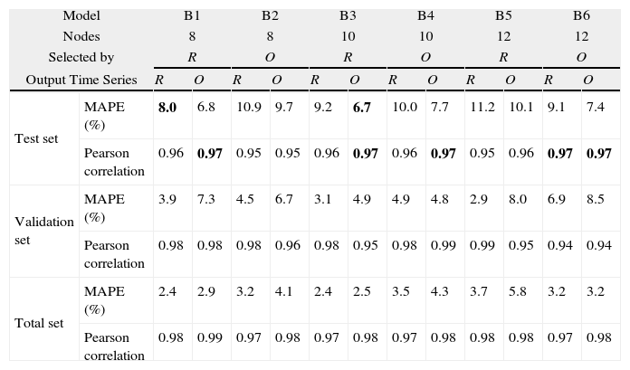
Table 4 presents the MAPE and Pearson correlation for Model B with 8, 10 and 12 nodes in the hidden layer. The weights matrix of the ANN was selected along the 50 training sessions by the lower MAPE in the validation set of one of the outputs (R or O) defined in the row ‘selected by’.
Performance of sub-models B.
| Model | B1 | B2 | B3 | B4 | B5 | B6 | |||||||
| Nodes | 8 | 8 | 10 | 10 | 12 | 12 | |||||||
| Selected by | R | O | R | O | R | O | |||||||
| Output Time Series | R | O | R | O | R | O | R | O | R | O | R | O | |
| Test set | MAPE (%) | 8.0 | 6.8 | 10.9 | 9.7 | 9.2 | 6.7 | 10.0 | 7.7 | 11.2 | 10.1 | 9.1 | 7.4 |
| Pearson correlation | 0.96 | 0.97 | 0.95 | 0.95 | 0.96 | 0.97 | 0.96 | 0.97 | 0.95 | 0.96 | 0.97 | 0.97 | |
| Validation set | MAPE (%) | 3.9 | 7.3 | 4.5 | 6.7 | 3.1 | 4.9 | 4.9 | 4.8 | 2.9 | 8.0 | 6.9 | 8.5 |
| Pearson correlation | 0.98 | 0.98 | 0.98 | 0.96 | 0.98 | 0.95 | 0.98 | 0.99 | 0.99 | 0.95 | 0.94 | 0.94 | |
| Total set | MAPE (%) | 2.4 | 2.9 | 3.2 | 4.1 | 2.4 | 2.5 | 3.5 | 4.3 | 3.7 | 5.8 | 3.2 | 3.2 |
| Pearson correlation | 0.98 | 0.99 | 0.97 | 0.98 | 0.97 | 0.98 | 0.97 | 0.98 | 0.98 | 0.98 | 0.97 | 0.98 | |
Therefore 6 sub-models were experimented. Sub-models B1 and B2 were 8 hidden nodes, submodels B3 and B4 10 hidden nodes and sub-models B5 and B6 12 hidden nodes. Sub-models B1, B3 and B5 had the weights matrix selected by the minimization of MAPE in the Revenue output, meanwhile sub-models B2, B4 and B6 had the weights matrix selected by the minimization of MAPE in the Total Overnights output.
The Revenue was better predicted by sub-model B1 with MAPE of 8.0%, and Pearson correlation of 0.96 in test set. The Total Overnights for this sub-model presents a MAPE of 6.8% and r=0.97 that is very close to the better values for the Total Overnights prediction.
The Total Overnights was better predicted by sub-model B3 with MAPE of 6.7% and Pearson correlation of 0.97, although other sub-models reached the same value of Pearson correlation. The Revenue time series for this sub-model presented a MAPE=9.2% and an r=0.96.
The Revenue was better predicted by a model with the weights matrix selected by the Revenue, but now the Total Overnights was also better predicted by a model with weights matrix selected by the Revenue time series.
Model B demonstrated better behaviour to predict the Total Overnights than the Revenue because it has the previous data of Total Overnights in its entrance.
Considering validation and Total sets sub-model B1 and B3 still has good comparative performance for Revenue and Total Overnights, respectively.
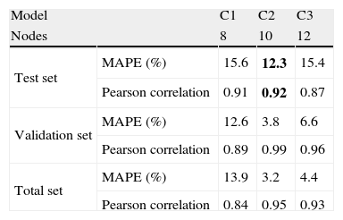
4.3Model CModel C is a dedicated ANN to the Revenue time series using the previous values in the input to predict the Revenue for the actual month. The model is similar to model A, but has only one output.
Sub-models C1, C2 and C3 have 8, 10 and 12 nodes in their hidden layers, respectively.
Table 5 shows the performance for sub-models C. Sub-model C2 presents a MAPE of 12.3% and a Pearson correlation r=0.92 in test set. Although the worst performance of this model in test set, the performance in the validation set and in the Total set is at similar level of previous models A and B, denoting some inability by the new data of test set. The low MAPE in validation and total sets shows some overfit to the training set but low generalization capacity.
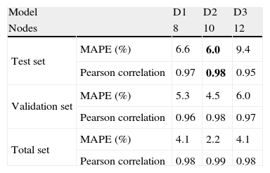
4.4Model DModel D is similar to model C; but now for the Total Overnights time series, sub-models D1, D2 and D3 have 8, 10 and 12 nodes in their hidden layers, respectively.
Contrary to model C this model D shows very good performance using 8 and 10 nodes in the hidden layer, as can be seen in Table 6. This model presented the lower MAPE for this time series with only 6% for model D2 and a Pearson correlation r=0.98, for the test set.
Considering the validation and Total sets the sub-model D2 still presents the better performance denoting high consistence along the several years of the time series.
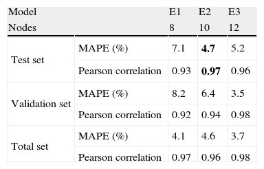
4.5Model EModel E is similar to models C and D; but now for the Domestic Overnights time series, sub-models E1, E2 and E3 have 8, 10 and 12 nodes in their hidden layers, respectively.
Table 7 presents the performance for these sub-models. A very high performance of this model E, particularly model E2 (10 nodes in hidden layer) with only 4.7% of MAPE and r=0.97, in test set, can be seen.
For the validation and Total sets sub-model E3 presents better performance than E2, denoting that the E3 with 12 nodes in the hidden layer does not show the same ability to generalize in test set as E2 with only 10 nodes in hidden layer.
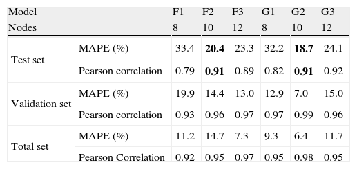
4.6Model FModel F is similar to model E but for Foreign Overnights. It uses the previous 12 months of the FO time series in the input to predict the actual month of the same time series. Sub-models F1, F2 and F3 have 8, 10 and 12 nodes in their hidden layers, respectively.
Table 8 presents the performance for sub-models F and G. Concerning sub-models F, it can be seen that sub-model F2 is the one with better performance with MAPE=20.4% and Pearson correlation of 0.91, in test set.
Performance of sub-models F and G.
| Model | F1 | F2 | F3 | G1 | G2 | G3 | |
| Nodes | 8 | 10 | 12 | 8 | 10 | 12 | |
| Test set | MAPE (%) | 33.4 | 20.4 | 23.3 | 32.2 | 18.7 | 24.1 |
| Pearson correlation | 0.79 | 0.91 | 0.89 | 0.82 | 0.91 | 0.92 | |
| Validation set | MAPE (%) | 19.9 | 14.4 | 13.0 | 12.9 | 7.0 | 15.0 |
| Pearson correlation | 0.93 | 0.96 | 0.97 | 0.97 | 0.99 | 0.96 | |
| Total set | MAPE (%) | 11.2 | 14.7 | 7.3 | 9.3 | 6.4 | 11.7 |
| Pearson Correlation | 0.92 | 0.95 | 0.97 | 0.95 | 0.98 | 0.95 |
Considering the validation and Total sets sub-model F3 presents better performance than the other sub-models. Anyhow both sub-models F2 and F3 present far better performance in validation and Total sets than in test set denoting a poor capacity of this model to generalize to never seen data.
4.7Model GModel G predicts the same Foreign Overnight time series, but now uses also the DGP of Spain, France and UK in the input besides the previous 12 months of the FO time series. Sub-models G1, G2 and G3 have 8, 10 and 12 nodes in their hidden layers, respectively.
Considering the performance of sub-models G presented in Table 8 it can be seen that the submodel G2 performs better with a MAPE of 18.7% and Pearson correlation of 0.91, in test set.
Regarding the validation and Total sets sub-model G2 still performs better than the other submodels, but again the G sub-models denoted poor ability to generalize to never seen data present in test set.
4.8Model HBecause previous models A, B and C did not show very good ability to predict the Revenue time series some other ANN models were experimented.
Model H predicts the Revenue time series and has in the input previous Total Overnights, actual Foreign Overnight and GDP of Portugal, Spain, France and UK. Sub-models H1, H2 and H3 have 8, 10 and 12 nodes in their hidden layers, respectively.
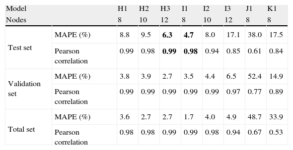
Table 9 presents the performance for sub-models H and I, and for models J and K to predict the Revenue time series using different input features.
Performance of sub-models H and I and models J and K.
| Model | H1 | H2 | H3 | I1 | I2 | I3 | J1 | K1 | |
| Nodes | 8 | 10 | 12 | 8 | 10 | 12 | 8 | 8 | |
| Test set | MAPE (%) | 8.8 | 9.5 | 6.3 | 4.7 | 8.0 | 17.1 | 38.0 | 17.5 |
| Pearson correlation | 0.99 | 0.98 | 0.99 | 0.98 | 0.94 | 0.85 | 0.61 | 0.84 | |
| Validation set | MAPE (%) | 3.8 | 3.9 | 2.7 | 3.5 | 4.4 | 6.5 | 52.4 | 14.9 |
| Pearson correlation | 0.99 | 0.99 | 0.99 | 0.99 | 0.99 | 0.97 | 0.77 | 0.89 | |
| Total set | MAPE (%) | 3.6 | 2.7 | 2.7 | 1.7 | 4.0 | 4.9 | 48.7 | 33.9 |
| Pearson correlation | 0.98 | 0.98 | 0.99 | 0.99 | 0.98 | 0.94 | 0.67 | 0.53 |
Considering the sub-models H of Table 9, it can be seen that sub-model H3 outperforms previous models with MAPE of 6.3% and Pearson correlation of 0.99, in test set.
Regarding the validation and Total sets sub-model H3 still has the better performance with the same Pearson correlation as in test set denoting very good ability to generalize with never seen input data.
4.9Model IModel I also predicts the Revenue time series but has the previous values of the Revenue time series in the input besides the actual Foreign Overnight and GDP of Portugal, Spain, France and UK. Sub-models I1, I2 and I3 have 8, 10 and 12 nodes in their hidden layers, respectively.
Considering the sub-models I of Table 9, it can be seen that sub-model I1 outperforms previous models with MAPE of 4.7% and Pearson correlation of 0.98, in test set.
Regarding the validation and Total sets sub-model I1 still has the better performance as in test set denoting very good ability to generalization with never seen input data.
This I1 sub-model presented very low MAPE in the task of prediction of the Revenue.
Models H and I have 17 input nodes which make difficult the training process with the Levenberg–Marquardt algorithm. Therefore the Resilient backpropagation algorithm was experimented in these models but with worst results. Six nodes in the hidden layer were also experimented with model H but also with worst results.
Because of memory problems during the training process models I2 and I3 were only 10 training sessions instead of the 50 training sessions used for all other models.
4.10Models J and KModels J and K also intend to predict Revenue time series but the input are simpler than in previous models. Namely model J has only 6 input nodes and does not use previous data in the input. Model K has only 3 input nodes for previous values of Revenue R(i−1), R(i−4) and R(i−12).
Both models were experimented with 8, 10 and 12 nodes in hidden layer, but the results were even worse than the ones presented in Table 9 for sub-models J1 and K1.
The MAPE for sub-model J1 is 38% and for sub-model K1 it is 17.5%. Regarding the validation and Total sets the performance is still awful. Therefore, these models showed no ability to predict this Revenue time series.
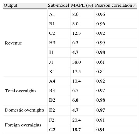
4.11Comparison of modelsComparing the best sub-model with the same output Table 10 resumes the best performance grouped by its output. Therefore, for the Revenue time series the sub-model I1 can be considered the one with best performance achieving the MAPE of 4.7% and r of 0.98. For the Total overnights time series the sub-model D2 is clearly the best model with MAPE of 6.0% and r=0.98. For the Domestic Overnights time series only one Model has been experimented because it achieved a good performance. Namely the sub-model E2 had a MAPE of 4.7% and r=0.97. The Foreign Overnights time series was better predicted with sub-model G2 with MAPE of 18.7% and r=0.91.
Performance of best sub-models.
| Output | Sub-model | MAPE (%) | Pearson correlation r |
| Revenue | A1 | 8.6 | 0.96 |
| B1 | 8.0 | 0.96 | |
| C2 | 12.3 | 0.92 | |
| H3 | 6.3 | 0.99 | |
| I1 | 4.7 | 0.98 | |
| J1 | 38.0 | 0.61 | |
| K1 | 17.5 | 0.84 | |
| Total overnights | A4 | 10.4 | 0.92 |
| B3 | 6.7 | 0.97 | |
| D2 | 6.0 | 0.98 | |
| Domestic overnights | E2 | 4.7 | 0.97 |
| Foreign overnights | F2 | 20.4 | 0.91 |
| G2 | 18.7 | 0.91 |
Several ANN models were experimented with the objective to forecast the tourism demand time series given by the monthly Revenue and Overnights. The Overnights could be considered as Total, Domestic and Foreign Overnights. The input of the models could be the previous months of the same time series or even the other time series, and/or the GDP of the most contributing countries for Portuguese tourism, namely Portugal, Spain, France and UK. Different combinations of input features were experimented in models with also different number of nodes in the hidden layer.
Models A and B have two nodes in the output to predict simultaneously both time series, Revenue and Total Overnights. Anyhow none of the sub-models A or B reached the best performance for any of the outputs.
The dedicated models C, D, E and F have the previous months of the output time series in their entrance. These models had very good results for Total Overnights and Domestic Overnights time series.
Considering the Prediction of the Revenue time series the best sub-model was model I1 reaching a MAPE of only 4.7% and a Pearson correlation coefficient of 0.98. This model has the previous values of the same time series, the present Foreign Overnights and the GDP of Portugal, Spain, France and UK in its entrance and has 8 nodes in the hidden layer. Model H3 reached also very good performance for this time series and the entrance also uses the Foreign Overnights and GDP of the same countries. This situation indicates the importance of these parameters together as the previous values of the same time series.
Concerning the prediction of the Total Overnights time series sub-model D2 behaves better than other models with a MAPE of 6.0% and r=0.98. This model has the previous 12 values of the same time series in their entrance. It is a similar model as the ones already tested in previous works like in Fernandes et al. (2008) with a different period of the time series but with a MAPE between 6.9 and 8.7% depending on the year and region. The difference between model B and D is that model D has only one output and model B has two outputs denoting a better behaviour of the ANN when it is dedicated to only one objective.
Considering Domestic Overnights only model E has experimented because it achieved good results with the sub-model E2. The MAPE has 4.7% and r=0.97. This model also has the previous values of the time series in its entrance, similar to model D2.
The prediction of Foreign Overnights seem to be most difficult because the best sub-model G2 only achieved a MAPE of 18.7% and r=0.91. This model has the previous 12 values in the entrance as in sub-model F2 but also includes the GDP of the most tourism contributing countries, namely Spain, France and UK, denoting the importance of these parameters in the entrance of the ANN.
Comparing the performance of models used to predict Domestic and Foreign Overnights it seem clear that Domestic Overnights are more predictable than Foreign Overnights, and that Foreign Overnights are dependent of the GDP of contributing countries.
As a final conclusion ANN based models proved once again their good ability to forecast tourism time series.
João Paulo Teixeira (Ph.D. in Electrical and Computers Engineering) is an adjunct professor of the Electrical Department in the School of Technology and Management in the Polytechnic Institute of Bragança (IPB). His research interests include: Modeling, Artificial Neural Network, Signal Processing and Speech Processing.
Paula Odete Fernandes (Ph.D. in Applied Economics and Regional Analysis) is a professor of management, in the Polytechnic Institute of Bragança (IPB) – Portugal. She is a researcher of NECE (UBI) and Scientific Coordinator of UNIAG (Applied Management Research Unit). Her research interests include: Tourism, Management, Artificial Neural Network, Entrepreneurship, Econometric Modeling, Marketing Research, and Applied Research Methods. She has participated in 4 international projects I&D and has more than 90 publications in proceedings and scientific journals with referee.
