An innovative high-frequency statistical arbitrage in Chinese futures market

Abstract

The primary use of futures is hedging risk. Traders in the spot market can hedge certain risks through the futures market. With the development of the futures market, the arbitrage transactions around futures have attracted increasingly attention. The aim of this paper is to establish an innovative and unique pairs trading framework, and use it to test the effectiveness of China's futures market. The framework for pairs trading is based on cointegration test, Kalman filter and Hurst index filtering. We use the data of 47 commodities with relatively good liquidity in the Chinese commodity futures market. We apply the representative index of China's commodity futures market, "Wenhua Commodity Index" as the benchmark, to evaluate the performance of the strategy and compare it with the benchmark model. This study found that, according to the pairs trading framework, after considering transaction costs, the cumulative return in the sample reached 81%, the cumulative return out of the sample was 21%. It is worth noting that the out-of-sample maximum drawdown achieved excellent results of no more than 1%. In the same period, trading the Wenhua Commodity Index with a "buy and hold" strategy achieved a gain of 31%, but with maximum drawdown reached 15%. The values of our paper are, first it proves that Chinese commodity futures market is not a weak-form efficient market, because technical analysis based on machine learning could obtain excess returns. Second, this research combines the theory and practice of statistical arbitrage, which also provides guiding significance for investment practice.

Introduction

Currently, the proportion of quantitative trading in the global financial market is increasing, and quantitative strategy models have received increasing attention from the financial industry. With the remarkable development of modern computer technology, proprietary trading departments of hedge funds and investment banks increasingly use statistical arbitrage strategies in the stock, foreign exchange, and futures markets (Gatev et al., 2006). Statistical arbitrage strategies were originally developed by applied mathematicians and computer engineers in the 1980s (Vidyamurthy, 2004). The pairing strategy examined in this study is a statistical arbitrage strategy, a mean-reversion strategy designed to profit from the mean-reversion behavior of a particular pairing ratio. The idea behind pairs trading strategies is to take advantage of the “price anomalies” created by market inefficiencies. The specific trading rule is to find two or more financial assets with the same price trend, observe the widening of the spread, buy them at a relatively low price, and sell them at a relatively high price. The trade will be profitable if the security converges toward its historical spread pattern. The assumption behind this strategy is that asset-pair spreads that exhibit cointegration properties are mean-reverting in nature, thus providing an arbitrage opportunity if the spread deviates significantly from the mean.

As an emerging developing country, China's financial market has flourished and matured since the beginning of the 21st century. Its futures and derivatives markets play essential roles in serving the real economy, providing hedging tools for spot companies, and enriching the allocation of financial assets by investment institutions. In 2021, China's futures market maintained good development momentum, with continued growth in scale and volume, and market construction deepened. From the perspective of market capacity and depth, the total funds in China's futures market exceeded 1.2 trillion RMB, an increase of 44.5%, by the end of 2020data from the China Futures Association in 2021. From the perspective of market breadth and degree of diversification, there are currently 94 types of futures options on the market, and the main products’ integrity has improved. The commodity futures market is integral to the futures and derivatives market. Therefore, this study focuses on China's commodity futures market and uses intraday and minute-level data to study the performance of statistical arbitrage. The main reasons why we specialize in China's commodity futures market are as follows: First, no short-selling mechanism exists in China's stock market. Thus, there is no stock future, and only certain stocks can be shorted by “margin financing”. In most cases, we can only short stocks, which make stocks in the Chinese market unsuitable for pairs trading. Second, in the current Chinese futures market trading, the proportion of fully algorithmic trading is lower than that in developed countries, which provides a massive opportunity for quantitative arbitrage trading. On the contrary, in developed futures markets, arbitrage opportunities are not easily recognized, which means that opportunities may exist for those who seek and can take advantage of them. Finally, high-quality data plays a vital role in algorithmic trading. Many data service companies in China, such as Wind and JoinQuant, provide excellent data interfaces. Through these data interfaces, we can access the daily main contract data for China's three major commodity futures exchanges.

This study develops an intraday high-frequency pairing strategy. It tests the strategy's performance in the Chinese commodity futures market, using the intraday minute-level data of 47 commodity futures with relatively good liquidity in the Chinese commodity futures market. The strategy consists of the following steps: First, we exhaust the spread relationships among all commodity futures contracts in the sample. Second, through the cointegration test of the spread, we check whether a long-term co-movement relationship exists between commodities. Third, an Augmented Dickey-Fuller test is performed on the spread to confirm statistically whether the series is mean-reverting. Fourth, we calculate the Kalman Filter regression and lagged spread series on the spread series and use the coefficients to calculate the mean reversion half-life. Fifth, the Hurst index is used to evaluate the mean reversal characteristics of the spread. Sixth, according to the above filtering conditions, we select the appropriate commodity pairing, establish trading rules for opening and closing positions, and conduct algorithmic trading experiments. Finally, based on the representative index of China's commodity futures market, the “Wenhua Commodity Index,” the strategy's performance is evaluated and compared with the benchmark model.

The rest of this paper is arranged as follows. Section two is literature review part. Section three introduces the pairs trading framework of the commodity futures established in this study. Section four presents the algorithmic trading rules and trading performance evaluation. The data used in this study is explained in Section five. Moreover, section six is the discussion part. Section seven is the conclusion.

Literature review

In recent years, the statistical arbitrage strategy in quantitative trading has become increasingly popular in academia and the investment industry, for example, the copula model (Zeng et al., 2023), BP-GRACH (Hou et al., 2020), and pairs trading strategy (Chen et al., 2022; Lee, 2022; Zhao, 2022). Early arbitrage studies mainly investigated the risk-free arbitrage strategies of futures contracts traded in different markets, to examine the market efficiency (Dunis et al., 2010; Fung et al., 2010). After that, some developed countries have begun to involve exchange-traded funds (ETFs) in their financial markets, verifying the effectiveness of this strategy on ETFs (Clegg & Krauss, 2018). Nevertheless, there is relatively limited discussion on risk arbitrage, especially in the existing literature, which seldom considers the factors of transaction and impact cost (Chan, 2021). Gatev et al. (1999) first proposed the risk arbitrage analysis of financial assets, particularly the pairs trading analysis. Luo and Dan (2021) also found that the most typical statistical arbitrage strategy in the securities and futures market is the pairs trading strategy. Based on previous literature, we found that, research on pairs trading in the commodity futures market is relatively rare and mostly limited to the stock market. For example, Bai and Slepaczuk (2022) applied the pairs trading method in S&P 500 index in the US stock market. Chen et al. (2022) used the pairs trading method to test the returns on 44 stocks selected from the Taiwan 50 Index. Lee (2022) analyzed the S&P 500 and Russell 2000 indices by using pairs trading strategy. The complexity of futures market determines the difficulty of its research. Compares to the stock market, commodity futures market has higher leverage and risk associated with the contracts, as well as the need to consider the impact of factors such as seasonality and basis variation.

Currently, the research on the pairs trading of commodity futures market mainly focuses on the following aspects. Firstly, some studies focused on the methodology and feasibility study of the effectiveness of statistical arbitrage strategies and the stability of arbitrage models. Wang (2021) discussed the theoretical engineering implementation of the pairs trading in futures statistical arbitrage strategy. Above researches mainly focused on theoretical feasibility, and have not been combined with practice. Secondly, some literatures conducted a micro-level investigation of pairs trading—for example, the inter-temporal arbitrage (same pairs of goods in different periods). Du (2021) selected six soybean meal futures contracts of different months in the Dalian Futures Exchange. Moreover, the inter-market spread (different exchanges with the same pairs of goods and at the same periods). Furthermore, the inter-commodity spread (different pairs of goods at the same periods, same exchanges) such as soybean, soybean oil, and soybean meal futures (Huang & Wang, 2021), Coke futures and coking coal futures (Liu, 2020). These studies normally concentrate on the relationships between several paired commodities during a certain time period in the past, which is a historical study without reference significance for the future. They can only illustrate the performance of paired commodities in the past, and lack a holistic consideration for the whole market. Thirdly, some scholars focus on the impact of data frequency on pairs trading statistical arbitrage results, while most studies have focused on relatively low-frequency daily data (Avellaneda & Lee, 2010; Do & Faff, 2010;Gatev, 2006; Gatev et al., 1999; Liew & Wu, 2013; Vidyamurthy, 2004; Zhou, 2022). Compared to high-frequency data, low-frequency data can quickly narrow the price difference of spot arbitrage, resulting in fewer arbitrage opportunities and higher arbitrage costs.

Our research has further improved on the basis of existing literature. First, we develop an innovative trading framework for pairs trading based on cointegration test, Kalman filter and Hurst index filtering. Moreover, we combine the theory with practice, and backtest our strategy through huge amount of historical data and conduct it to simulation test. Furthermore, our research focuses on the meso level, we chooses 47 commodities with relatively good liquidity and value which can reflect the overall situation of the market. At last, we further refine the data frequency to minute-level high-frequency data on their basis to test the profitability of commodity futures market matching trading strategy. And to explore the market efficiency of this particular market type, asset class, and commodity futures contracts in the commodity futures market.

High-frequency pairing trading framework

This study conducts research according to the following steps: First, we use the data interface provided by JohnQuant to export the 5-minute price, trading volume, and other data of 47 primary commodities in China's commodity futures market for consecutive contracts to ensure that the data length of each commodity is the same; second, we conduct cointegration and ADF tests for each possible commodity pairing, examine the cointegration and stationarity of all paired commodities, and select potential paired commodity combinations with trading potential; third, the price difference of potential paired commodities; and for the mean regression test, we calculate the adaptive Hurst index to confirm whether the spread series is mean-regression in a statistical sense; fourth, we use Kalman filter regression on the spread series and the lagged series of the spread series, using the Kalman filter, and the regression coefficient is used to evaluate the half-life of the mean regression. Fifth, we normalize the spread, calculate the Z-score of the trading signal, and define the entry and exit Z-score levels for backtesting. The theoretical and technical roadmap of this study shows in Fig. 1.

Fig. 1.

The theoretical and technical roadmap of this study

Source: Made by author.

Cointegration test of spread

The pairs trading strategy concept comes from identifying a stationary price series. Following Engle and Granger's (1987) method, if two non-stationary price series are integrals of order 1, that is, I (1), considering that the first-order difference of the price series is stationary, that is, I (0), then there is a linear combination of the series, forming a stationary process, making the price series known as first-order cointegration.

Where yt and xt are the cointegrated price series, β is the cointegrated coefficient, and et is the stationary cointegration error. Under this framework, the cointegrated price series presents a long-term equilibrium relationship, and any deviation from this equilibrium is corrected in the short term, which can be represented by an error correction model (ECM) in the following form:

Where εyt is the stationary error, and long -term errors αy and αx in estimated coefficients reflect that price series will adjust their equilibrium paths in the short term according to their long-term balance paths or how quickly they adjust. The mean reversion property of cointegration aligns with the pairs trading concept, and some studies have integrated this concept into pairs trading strategies (Vidyamurthy, 2004). In this study, we employ a cointegration framework and an ECM to estimate the long-run equilibrium relationships between pairs of securities. In addition, we detect deviations in paired commodity spreads from long-term equilibrium relationships, a procedure commonly used to signal long or short positions in financial asset pairing transactions. Meanwhile, the estimated eigenvectors use the Johansen cointegration test (Johansen, 1995) as the arbitrage ratio to determine the portfolio weights:

The spread is defined by the following formula:

The Z-score has a standard normal distribution and helps determine the normalized deviation of the long-term relationship. The following method is adopted to estimate the deviation from the spread:

Kalman filter and dynamic arbitrage ratio

We use a Kalman filter to calculate the dynamic arbitrage ratio. In pairs trading, after the potential trading commodity pairing is confirmed using cointegration and stationarity tests, the hedge ratio of the trading pairs and the statistical characteristics of its residual sequence need to be determined, which determines the strategy's feasibility and the formulation of trading rules. These parameters often change dynamically with time in the actual transaction process and must be estimated and adjusted over time. In the literature, calculating the sample's statistical characteristics in the sliding window is usually used for estimation, or unequal weighting schemes such as exponential smoothing moving average are applied to increase the influence of newer information. However, choosing the optimal proportioning scheme is also a complex problem. The Kalman filter can be applied to the dynamic estimation of parameters in pairs trading because of its characteristics and powerful and flexible methods.

The Kalman filter is also called the Linear Quadratic Estimation (LQE) algorithm, and its principle is as follows. Unobservable variables exist in economic and financial systems that can affect the real economic state, that is, the state vector. The model containing the state vector cannot be solved directly and must be solved using the state space. Let y_t be a k-dimensional observation vector containing k variables, let m-dimensional state vector a_t be related to y_t, state vector a_t is unobservable, and the state space model has the following form:

Where εt and vt are the disturbance vectors obeying the normal distribution; is the first-order vector autoregressive process; and (9) and (10) become the signal and the state equations, respectively.

Considering the conditional distribution of the state vector αt at time s, the mean and variance matrices of the conditional distribution can be defined as:

By estimating the joint probability distribution of the variables for each period, the estimates of unknown variables tend to be more accurate than estimates based on a single measurement alone. Because Kalman filtering updates its estimates at each time step and tends to trade off recent observations over older ones, a practical application is estimating data rolling parameters. When using a Kalman filter, the window length must not be specified. The algorithm was first used to solve system control problems in engineering. Time-varying systems are assumed to transition linearly from one system state to the next, and each state is described by a set of system parameters. During the system state transition, the changes in these parameters were assumed to be linear. The typical Kalman filtering process is divided into three steps: 1. prediction; 2. observation; 3. correction.

Assuming that we obtained the estimated values of the system parameters in the current state, we can predict the predicted values of these parameters in the next state according to a certain linear model. We then let the system run for some time and enter the next state to observe the system. Owing to the existence of errors and randomness, we can only obtain the observed values of some variables related to the system parameters (typically the potential system variables plus random items). Finally, combined with the information on the relevant variables’ observed values, the system parameters’ predicted values are corrected under a certain rule to obtain the estimated values of the system parameters in the new state. Over time, the system constantly changes to a new state, and the system parameters are continuously estimated dynamically.

Kalman filtering is a recursive filtering algorithm originally used to guide the navigation and guidance systems of the Apollo lunar spacecraft. Compared with other filtering models, the advantages of Kalman filter are very prominent:

First, Kalman filter can be used in nonlinear systems and is easy to implement. Although Particle Filter and Extended Kalman Filter can also deal with nonlinear problems, however the computational cost in high-dimensional systems is high. Second, Kalman Filter can adapt to system noise and measurement error. Although the filtering methods such as Wavelet Filter and Median Filter can also be used to remove outliers, but they cannot estimate the system state. Adaptive Kalman Filter can handle time-varying system parameters, but it requires prior knowledge of the system model. Machine learning methods such as Neural Networks, Decision Trees, and Support Vector Machines do not require prior knowledge of the system model, but require a large amount of training data to optimize algorithms and reduce errors. Third, Kalman filtering can obtain the optimal solution while possessing the covariance information of the solution. Fourth, it can effectively address the issue of excess in online computing processes. In summary, we use Kalman filter to calculate the dynamic arbitrage ratio.

Hurst index and spread mean reversion

Based on the cointegration test, we apply an additional mean-reversion effect test to the spread of paired commodities using the Hurst exponent to filter out spurious mean-reversion signals (Ramos-Requena et al., 2017). The Hurst index is used as a measure of the long-term memory of a time series, which is related to the autocorrelations of the time series and the rate at which these correlations decline as the lag between the paired values increases. According to the definition of the Hurst index, when H is less than 0.5, the spread is inversely persistent; when H is greater than 0.5, the spread is persistent; and when H is equal to 0.5, the spread is a white noise process. For commodity pairs that pass the cointegration test, the Hurst index of the price difference must be less than 0.5, which can filter out price differences that pass the cointegration test but do not have the characteristics of mean-reversion. Simultaneously, it is helpful to sort commodity pairing combinations according to the size of the Hurst index.

The main methods for calculating the Hurst index are as follows: Hurst (1951) proposed the rescaled range (R/S) method, periodogram regression (Geweke & Hudak, 1983; wavelet analysis (Holschneider, 1988), multifractal castration fluctuation analysis (Peng et al., 1994); Kantelhardt et al., 2002), among others. Among these, castration volatility analysis (Peng et al., 1994), a common method for calculating the Hurst index, is used to analyze the complexity and randomness of financial time series. The advantage of this method is that it detects long-range correlations in nonstationary time series while avoiding false positives. However, when the DFA method divides the sequence, the boundaries of the adjacent line segments are discontinuous. The DFA may not be a good choice if the sequence has a trend, non-stationarity, or nonlinear oscillation characteristics (seasonal). The newly emerging adaptive fractal analysis (AFA) method can overcome the DFA method's shortcomings. The procedure for calculating the Hurst index using the AFA method is as follows.

Construct a random walk process from a sequence {x1,x2,x3,…,xN}:

The global smooth trend v(i)with respect tou(i) is obtained using adaptive filtering, given by:

Solve for H, which is Hurst Index (Riley et al., 2012).

Data interpretation and algorithmic trading

Data description

As of December 2021, China's commodity futures market has 64 contracts. To replicate the real trading environment, we obtained the intraday closing price and trading volume of 47 commodity futures price indices with a 5-minute frequency from JoinQuant. The amount of data is relatively large, so we set the sample data from January 4, 2019, to December 30, 2021, each with a total of 22,455 observations. Since periods of market turmoil may lead to abrupt changes in the structure of commodity futures prices and spread series, for example, structural breakouts caused by high volatility can produce jumps in a price series (Fung et al., 2010). Therefore, this study's sample includes the outbreak of COVID-19 at the end of 2019 and the period of surge in commodity prices since May 2020— especially the price slump and surge in the Chinese commodity futures market before and after the epidemic, which makes the sample more representative. Earlier studies have shown that pairs trading performance varies over time (Craig & Krauss, 2018; Do & Faff, 2010; Gatev et al., 2006). However, these studies are usually based on period-by-period analysis. Therefore, we tested the in-sample and out-of-sample performance of the strategies at different time stages separately, which allowed us to examine the performance of the strategies at different market stages. Specifically, we divided the entire sample into two sets of backtests: the first set of 17,963 observations (9:00 on December 9, 2019, to 14:55 on August 3, 2021, accounting for 80% of the total period) is the in-sample backtest period, and the remaining 8981 observations (from 9:00 on August 4, 2021, to 14:55 on December 29, 2021, accounting for 20% of the total period) are the out-of-sample backtest period. The first 13,472 observations of the second group (9:00 on December 9, 2019, to 14:55 on March 9, 2021, accounting for 60% of the total period) are the in-sample backtest period. The remaining 4490 observations (3 from 9:00 on December 10 to 14:55 on December 29, 2021, accounting for 40% of the total cycle) are the out-of-sample backtest period.

The motivation for our research using intraday, minute-level data is as follows. First, if the frequency of the data is high, the pair trade entry and exit signal settings can be more precise, leaving room for higher profit margins. Second, we can find intraday averages that cannot be found in the low-frequency data scenario; third, using high-frequency data increases data samples, enabling the training of complex predictive models with reduced risk of overfitting. Finally, due to differences in commodity trading time, some contracts have night trading, so we adjusted the research sample time to the daily trading data of all sample commodities and uniformly deleted the night trading data and missing value samples. Therefore, the actual sample span is from December 9, 2019, to December 29, 2021, and there is a total of 45 5-minute high, open, low, close, volume, and open interest data on each trading day.

Because a single futures contract has expiration date, splicing contracts to construct a continuous price series is a difficult problem in basic data processing. Usually, adjacent futures contracts are rolled forward, that is, only holding futures contracts with the most recent expiry date to construct a continuous time series of futures prices is a common way (Li et al., 2017). However, in practice, such splicing contracts still encounter “price gaps.” which is not the best solution. To avoid the problem of data discontinuity caused by contract splicing, we directly use the commodity price indices provided by JoinQuant to generate continuous time-series futures prices, which can avoid the disadvantage of using different methods to splice contracts while maintaining the trend structure of each commodity.

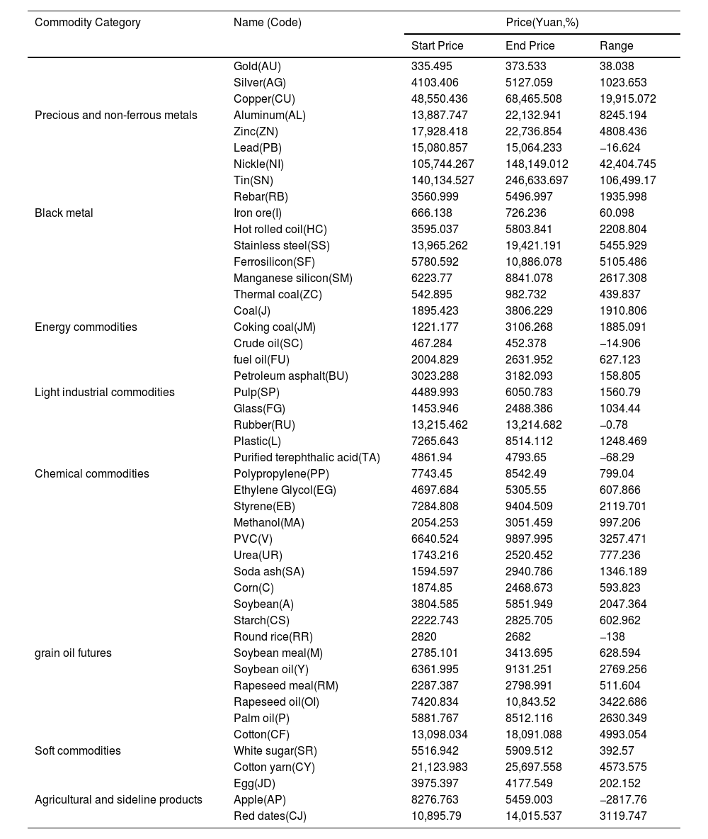
All commodity futures include eight precious and non-ferrous metals (gold, silver, copper, aluminum, zinc, lead, nickel, and tin); six ferrous metals (rebar, iron ore, hot rolled coil, stainless steel, ferrosilicon, and manganese silicon); six energy futures (coal, coking coal, thermal coal, crude oil, fuel oil, and petroleum asphalt); two light industrial commodities (glass and pulp); ten chemical commodities (rubber, plastic, purified terephthalic acid, polyvinyl chloride, ethylene glycol, methanol, polypropylene, styrene, urea, soda ash); nine grain oil futures (corn, soybean, starch, soybean meal, round rice, soybean oil, rapeseed meal, rapeseed oil, and palm oil); three soft commodities (cotton, white sugar, and cotton yarn); and three agricultural and sideline products (eggs, apples, and red dates). Table 1 lists the categories, names, exchange numbers, starting times, starting market prices, ending market prices, and changes in the sample period of the 47 commodity futures contracts. Within the sample range, the price changes in various commodity futures vary greatly, some of which have experienced sharp rises. Coking coal, coal, ferrosilicon, soda ash, thermal coal, tin, and hot-rolled coils have increased by over 60%, of which coking coal has increased by over 154%, the price of coke has increased by 100%, and the price doubles. Of the 47 products, 37 increased by over 10%, accounting for 79%. However, some commodity prices fluctuate cyclically until the end date remains almost unchanged from the start date. The increase in petroleum asphalt, eggs, and rubber is less than 5%, and the prices of some commodities have fallen. Negative growth occurred during the sample period in which the price of apples fell by 34%. In general, the sample period covers the period of rising commodity prices from May 2020. Commodities with large price increases are ferrous metals and energy commodities, and commodities that have fallen are mainly agricultural and sideline products. The sample period also includes the regulatory period of China's State Council for the rapid rise in commodity futures prices from May 2021. The sample time range includes the rising and falling trends of commodities and the market volatility caused by policy shocks, so it is representative to a certain extent.

Table 1.

Commodity futures contract, commodity price during the sample period.

Commodity Category	Name (Code)	Price(Yuan,%)
		Start Price	End Price	Range
	Gold(AU)	335.495	373.533	38.038
	Silver(AG)	4103.406	5127.059	1023.653
	Copper(CU)	48,550.436	68,465.508	19,915.072
Precious and non-ferrous metals	Aluminum(AL)	13,887.747	22,132.941	8245.194
	Zinc(ZN)	17,928.418	22,736.854	4808.436
	Lead(PB)	15,080.857	15,064.233	−16.624
	Nickle(NI)	105,744.267	148,149.012	42,404.745
	Tin(SN)	140,134.527	246,633.697	106,499.17
	Rebar(RB)	3560.999	5496.997	1935.998
Black metal	Iron ore(I)	666.138	726.236	60.098
	Hot rolled coil(HC)	3595.037	5803.841	2208.804
	Stainless steel(SS)	13,965.262	19,421.191	5455.929
	Ferrosilicon(SF)	5780.592	10,886.078	5105.486
	Manganese silicon(SM)	6223.77	8841.078	2617.308
	Thermal coal(ZC)	542.895	982.732	439.837
	Coal(J)	1895.423	3806.229	1910.806
Energy commodities	Coking coal(JM)	1221.177	3106.268	1885.091
	Crude oil(SC)	467.284	452.378	−14.906
	fuel oil(FU)	2004.829	2631.952	627.123
	Petroleum asphalt(BU)	3023.288	3182.093	158.805
Light industrial commodities	Pulp(SP)	4489.993	6050.783	1560.79
	Glass(FG)	1453.946	2488.386	1034.44
	Rubber(RU)	13,215.462	13,214.682	−0.78
	Plastic(L)	7265.643	8514.112	1248.469
	Purified terephthalic acid(TA)	4861.94	4793.65	−68.29
Chemical commodities	Polypropylene(PP)	7743.45	8542.49	799.04
	Ethylene Glycol(EG)	4697.684	5305.55	607.866
	Styrene(EB)	7284.808	9404.509	2119.701
	Methanol(MA)	2054.253	3051.459	997.206
	PVC(V)	6640.524	9897.995	3257.471
	Urea(UR)	1743.216	2520.452	777.236
	Soda ash(SA)	1594.597	2940.786	1346.189
	Corn(C)	1874.85	2468.673	593.823
	Soybean(A)	3804.585	5851.949	2047.364
	Starch(CS)	2222.743	2825.705	602.962
	Round rice(RR)	2820	2682	−138
grain oil futures	Soybean meal(M)	2785.101	3413.695	628.594
	Soybean oil(Y)	6361.995	9131.251	2769.256
	Rapeseed meal(RM)	2287.387	2798.991	511.604
	Rapeseed oil(OI)	7420.834	10,843.52	3422.686
	Palm oil(P)	5881.767	8512.116	2630.349
	Cotton(CF)	13,098.034	18,091.088	4993.054
Soft commodities	White sugar(SR)	5516.942	5909.512	392.57
	Cotton yarn(CY)	21,123.983	25,697.558	4573.575
	Egg(JD)	3975.397	4177.549	202.152
Agricultural and sideline products	Apple(AP)	8276.763	5459.003	−2817.76
	Red dates(CJ)	10,895.79	14,015.537	3119.747

Source: Data collect from JoinQuant.

Trading rules and performance evaluation

Backtesting is an essential aspect of formulating a trading strategy. It tests algorithmic trading rules using historical data, examines the strategy's performance in backtesting, and optimizes the trading rules to optimize and enhance the strategy. When backtesting the trading strategy's performance, only the data available at the time of the transaction is used, to avoid the problem of “data snooping” and avoid introducing future data in advance. For example, suppose a trading position is simulated based on daily low and high prices observed on the same day. In that case, it will reduce the accuracy of the real performance of the trade, as it is impossible to observe daily low and high prices until the end of the trading day. We can avoid look-ahead bias by dividing the dataset into two subsets: an in-sample dataset and an out-of-sample dataset. Therefore, the coding of arbitrage ratio spreads and other parameter calculations are based on different periods. In a typical backtesting framework, algorithmic trading is implemented one year after calculating the arbitrage ratio using the training set. Benefiting from the extensive application of information technology in the financial field, we can complete transaction backtesting on commercial-level quantitative trading platforms or open-source quantitative trading backtesting libraries. When our trading rules are coded, trading options can be backtested, and all combinations of preset parameters analyzed to find the best-performing rules. With a sufficient number of combinations, rules can be established to ensure good performance. However, extensive searches for variable combinations of different parameters can lead to a data snooping bias, another backtesting bias. The likelihood of achieving performance results purely through luck increases with the number of test combinations. Any trading rule that perfectly fits its sample data through backtesting may not yield the same performance when run on another dataset, resulting in a loss of performance durability. The entry-level of the z-score and window size of the diffusion moving average were estimated using both in-sample and out-of-sample datasets to minimize the probability of snooping bias. Two parameters, the entry-level of the z-score and the moving average window size of the diffusion were estimated using the in-sample and out-of-sample datasets to minimize the probability of snooping bias.

Gatev et al. (2006) used the spread of stock pairings to construct an arbitrage trading range, and the mean of the spread in the training set indicates the historical equilibrium of the spread. By setting the spread's upper and lower standard deviations as the threshold, when the spread crosses upwards and returns to the double standard deviation range of the spread, or vice versa, it triggers the trading of long assets with weaker trends and short assets with strong trends. The long and short positions are closed separately when the spread reverts and touches its historical average.

In this study, we draw on the trading ideas proposed by Gatev et al. (2006) to design the rules of high-frequency pairing trading in China's commodity futures market. The implementation steps of the trading rules are described as follows.

• (1)

  We obtain the daily closing prices and trading volumes of 47 commodity futures price indices with a frequency of 5 min from JoinQuant.

• (2)

  By using the sample data, first perform the ADF test to examine the stationarity of the spread. Secondly, perform cointegration testing. The paired products that can pass the ADF test and cointegration test are potential paired product combinations and the remaining are excluded.

• (3)

  Calculate the spread for each potential pairs (Spread = Y - Arbitrage Ratio*X).

• (4)

  Calculate the arbitrage ratio using the Kalman filter regression function.

• (5)

  Calculate the Hurst exponent and normalize the “spread” using the rolling mean and standard deviation of the period of the “half-life” interval to obtain a z-score.

• (6)

  Calculate the half-life using the half-life function.

• (7)

  We take the upper Z-score=2.0 and the lower Z-score=2.0, of the normalized spread as the opening threshold and Z-score=0 as the exit threshold.

• (8)

  When the normalized spread crosses the upper Z-score upwards, it opens a position to shorten the spread and closes the position when the Z-score returns to the exit position.

• (9)

  When the normalized spread crosses the lower Z-score downwards, it opens a long position and closes it when the Z-score returns to the exit position.

• (10)

  Backtest each commodity pair and calculate algorithmic trading performance, such as the annualized return and Sharpe ratio.

• (11)

  Build a portfolio of equivalent market value distributions, with each pair having the same market value.

The performance of this study's pairs trading strategies is measured by cumulative compound returns and Sharpe ratios:

where N is the decision criterion,−1 is short, 1 is long, H is the normalized hedge ratio, and R is asset return.

Empirical analysis

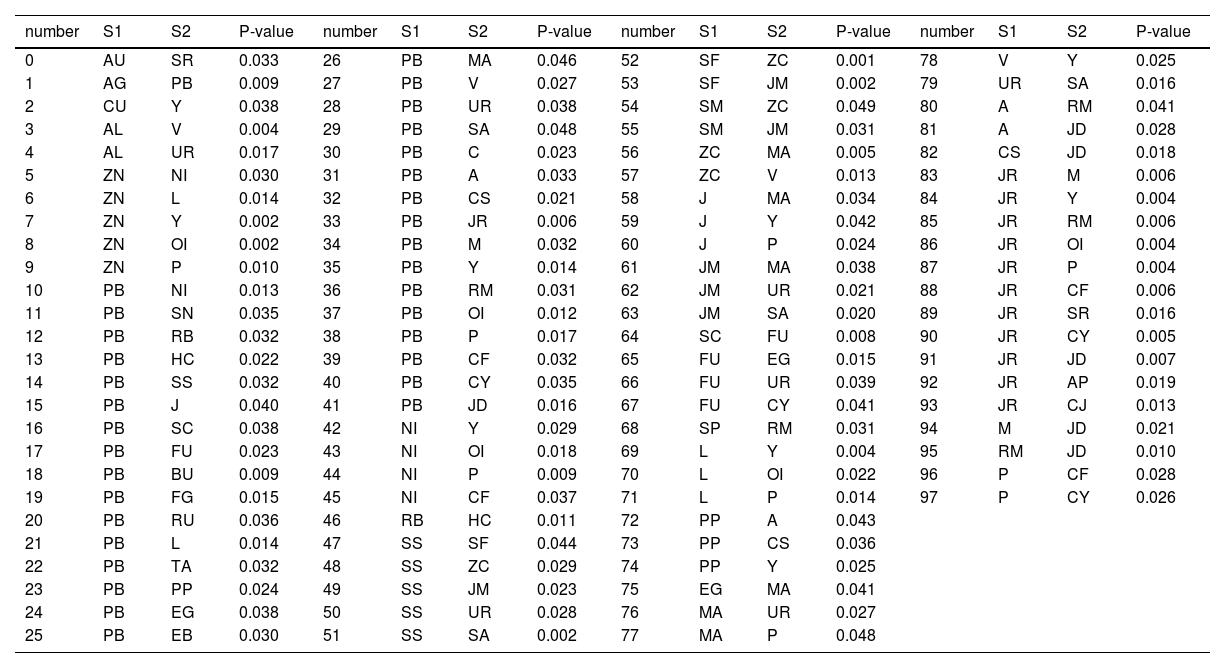
Our sample includes 47 commodities, with 1081 commodity pairing possibilities. Suppose we use intraday minute-level data for backtesting all commodity pairing possibilities. In that case, the computational overhead will be high, and there will also be many commodity pairing combinations without transaction potential. Therefore, applying filter conditions to all commodity combinations is necessary to filter out valuable paired commodity combinations. In this study, we filter out the paired combinations that fail the test through cointegration and ADF tests. Our goal is to identify two synchronous commodities; that is, the prices of the two commodities have changed roughly simultaneously in history. We filter according to the statistical test and obtain 95 potential commodity pairs with statistical arbitrage significance or in line with industrial logic. Table 2 lists all potential commodity pairs and the corresponding P value of the cointegration test. Potential commodity pairing includes the pairing combination of three types of relationships. First, the combination of coking coal (JM) and stainless steel (SS), which reflects the relationship between the upstream and downstream of the industrial chain; second, the combination that reflects the relationship between commodity categories, such as rebar (RB) and hot-rolled coil (HC); and third, commodity pairings, such as copper (CU) and soybean oil (Y), which have no industrial relationship and do not belong to the same commodity category. This feature reflects the advantages of statistical arbitrage; that is, it is entirely data-driven and based on the historical price difference between commodities.

Table 2.

Cointegration test and list of all potential paired commodities.

number	S1	S2	P-value	number	S1	S2	P-value	number	S1	S2	P-value	number	S1	S2	P-value
0	AU	SR	0.033	26	PB	MA	0.046	52	SF	ZC	0.001	78	V	Y	0.025
1	AG	PB	0.009	27	PB	V	0.027	53	SF	JM	0.002	79	UR	SA	0.016
2	CU	Y	0.038	28	PB	UR	0.038	54	SM	ZC	0.049	80	A	RM	0.041
3	AL	V	0.004	29	PB	SA	0.048	55	SM	JM	0.031	81	A	JD	0.028
4	AL	UR	0.017	30	PB	C	0.023	56	ZC	MA	0.005	82	CS	JD	0.018
5	ZN	NI	0.030	31	PB	A	0.033	57	ZC	V	0.013	83	JR	M	0.006
6	ZN	L	0.014	32	PB	CS	0.021	58	J	MA	0.034	84	JR	Y	0.004
7	ZN	Y	0.002	33	PB	JR	0.006	59	J	Y	0.042	85	JR	RM	0.006
8	ZN	OI	0.002	34	PB	M	0.032	60	J	P	0.024	86	JR	OI	0.004
9	ZN	P	0.010	35	PB	Y	0.014	61	JM	MA	0.038	87	JR	P	0.004
10	PB	NI	0.013	36	PB	RM	0.031	62	JM	UR	0.021	88	JR	CF	0.006
11	PB	SN	0.035	37	PB	OI	0.012	63	JM	SA	0.020	89	JR	SR	0.016
12	PB	RB	0.032	38	PB	P	0.017	64	SC	FU	0.008	90	JR	CY	0.005
13	PB	HC	0.022	39	PB	CF	0.032	65	FU	EG	0.015	91	JR	JD	0.007
14	PB	SS	0.032	40	PB	CY	0.035	66	FU	UR	0.039	92	JR	AP	0.019
15	PB	J	0.040	41	PB	JD	0.016	67	FU	CY	0.041	93	JR	CJ	0.013
16	PB	SC	0.038	42	NI	Y	0.029	68	SP	RM	0.031	94	M	JD	0.021
17	PB	FU	0.023	43	NI	OI	0.018	69	L	Y	0.004	95	RM	JD	0.010
18	PB	BU	0.009	44	NI	P	0.009	70	L	OI	0.022	96	P	CF	0.028
19	PB	FG	0.015	45	NI	CF	0.037	71	L	P	0.014	97	P	CY	0.026
20	PB	RU	0.036	46	RB	HC	0.011	72	PP	A	0.043
21	PB	L	0.014	47	SS	SF	0.044	73	PP	CS	0.036
22	PB	TA	0.032	48	SS	ZC	0.029	74	PP	Y	0.025
23	PB	PP	0.024	49	SS	JM	0.023	75	EG	MA	0.041
24	PB	EG	0.038	50	SS	UR	0.028	76	MA	UR	0.027
25	PB	EB	0.030	51	SS	SA	0.002	77	MA	P	0.048

Source: Author calculations.

Owing to space limitations, we take the classic arbitrage of similar commodities—the paired combination of rebar (RB) and hot-rolled coil (HC) as an example to illustrate the logic of the trading rules in this study, as shown in Fig. 2. We standardize the rebar and hot-rolled coil prices and then calculate the price difference between the two. Because both rebar and hot-rolled coil belong to the black commodity sector, the production materials of their finished products are similar, and the two have a profound economic relationship. Therefore, the price behaviors of the two are very similar, and it was found that the two have a significant cointegration relationship through the cointegration test. Cointegration is a more subtle relationship than correlation. If two time series are cointegrated, then some linear combinations exist between them that vary around a mean. The combinations between them are related to the same probability distribution at all the time points. Because of the difference between the actual prices of the two, the arbitrage ratio is not a 1:1 relationship; that is, one long (10 ton) rebar and one short (10 ton) hot-rolled coil are short. Therefore, we use the Kalman filter regression function rate to calculate the arbitrage ratio of the two. Then, we calculate the Hurst index and normalize the spread using the rolling average and standard deviation of the period of the “half-life” interval; and finally draw the mean of the spread and the upper and lower thresholds for opening and closing positions twice for the standard deviation of the spread condition, see Fig. 2.

Fig. 2.

Matching combination of rebar (RB) and hot rolled coil (HC)

Source: JoinQuant.

From the 47 commodities in China's commodity futures market, applying the framework proposed in this study and filtering according to statistical tests, we obtain 95 potential commodity pairs with statistical arbitrage significance or in line with industrial logic. This study conducted detailed in-sample and out-of-sample trading performance evaluations for each commodity pair and combination. The out-of-sample performance also used to test the robustness of this study.

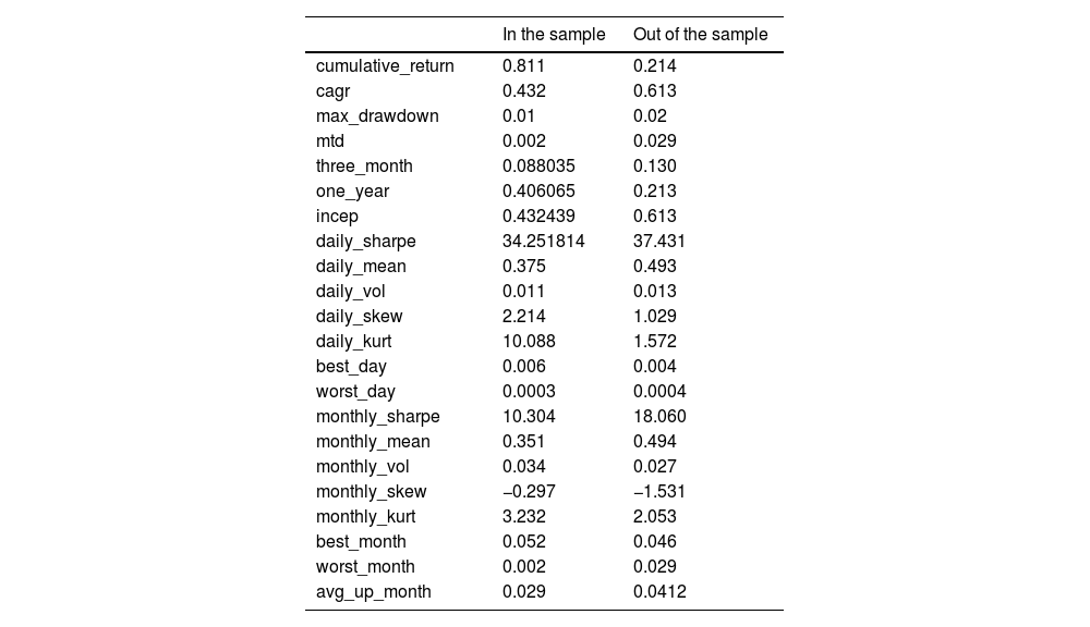
First, we report the in-sample trade performance of potential commodity pairings. Fig. 3 shows the cumulative returns of each commodity pair in the sample. Among the 95 commodity pairs, PB (lead)-AG (silver) achieved the highest cumulative return in the sample of 123.8%, a typical metal commodity pairing. The spread between the two commodities has an inherently stable mean-reversion mechanism. It is noteworthy that the commodity pairings such as JM (coking coal)-SS (stainless steel), methanol (MA)-urea (UR), and other commodity combinations with the highest cumulative yields have strong industrial background implications. Further, JM is the upstream commodity in the industrial chain of SS, and MA and UR are associated commodities that can be converted into each other. Meanwhile, lead (PB)-glass (FG), with the lowest cumulative return, is an unrelated commodity pairing. Based on the above results, using the arbitrage framework proposed in this study, the potential commodity pairs selected by the statistical arbitrage method can filter out most of the pairs that do not have the value of arbitrage transactions. Moreover, suppose we can combine the logic of arbitrage in the traditional industry chain. In that case, we can eliminate the matching combination of products that do not have industry chain relationships or irrelevant products from the potential matching products, which will be beneficial in improving the income of the matching combination of products. Fig. 4 shows the maximum in-sample drawdown of the net value of each commodity pair. The returns of each paired commodity in the sample are minimal, and the maximum return of the paired commodity with the largest average return is less than 3%. Because the positions of paired transactions are protected, for example, in a commodity pairing, if we are long in one commodity, we must short the other commodity. The source of profit is not the absolute change in price but the relative change in the price difference between commodities and the fluctuation of the price difference. The rate is much lower than the absolute change in commodity prices; therefore, the net value of the paired trades is relatively stable. Fig. 5 and Table 3 show how a portfolio consisting of all potentially paired commodities works within the sample. Within the sample, the net worth of the entire portfolio rises steadily, the net worth curve is smooth, and the drawdown is small. The cumulative return of the in-sample portfolio reaches 81.1%, and the maximum drawdown is less than 1%. The average daily Sharpe was 34.25, the monthly average Sharpe was 10.3, and the average daily income was 3.75%.

Fig. 3.

Intra-sample transaction performance of potential commodity pairings (December 9, 2019 9:00 to August 3, 2021 14:55)

Source: JoinQuant.

Fig. 4.

Maximum drawdown of returns within a sample of all potential commodity pairings. (December 9, 2019 9:00 to August 3, 2021 14:55)

Source: JoinQuant.

Fig. 5.

Commodity pairing portfolio in-sample trading performance and maximum drawdown. (December 9, 2019 9:00 to August 3, 2021 14:55)

Source: JoinQuant.

Table 3.

Performance statistics of algorithmic trading inside and outside the sample.

	In the sample	Out of the sample
cumulative_return	0.811	0.214
cagr	0.432	0.613
max_drawdown	0.01	0.02
mtd	0.002	0.029
three_month	0.088035	0.130
one_year	0.406065	0.213
incep	0.432439	0.613
daily_sharpe	34.251814	37.431
daily_mean	0.375	0.493
daily_vol	0.011	0.013
daily_skew	2.214	1.029
daily_kurt	10.088	1.572
best_day	0.006	0.004
worst_day	0.0003	0.0004
monthly_sharpe	10.304	18.060
monthly_mean	0.351	0.494
monthly_vol	0.034	0.027
monthly_skew	−0.297	−1.531
monthly_kurt	3.232	2.053
best_month	0.052	0.046
worst_month	0.002	0.029
avg_up_month	0.029	0.0412

Source: Author calculations.

Fig. 6 shows the cumulative return of each commodity pairing in an out-of-sample backtest. Among the 95 commodity pairs, the highest-yielding pairing is NI (nickel)-ZN (zinc). The out-of-sample cumulative return drops to 47.9%, which is also a typical metal commodity pairing, and has a solid industry chain arbitrage foundation. Commodity pairings with the highest cumulative returns also include rebar (RB)-lead (PB) and rapeseed oil (OI)-plastic (L). The commodity pairing with the lowest cumulative returns is eggs (JD)-corn starch (CS). The results of the out-of-sample pairing commodity returns are verified again. The pairing combination with a solid industry chain and pairing between related commodities has better pairing transaction returns. Fig. 7 shows the maximum out-of-sample drawdown of the net value for each commodity pair. Compared to the in-sample, the retracement of the net value of each commodity pairing is significantly expanded outside the sample, and the largest retracement of the commodity with the largest retracement reaches 5%. According to Table 3, the cumulative return of the out-of-sample portfolio decreases by 21.4%, and the maximum drawdown increases by 2%. The daily and monthly Sharpe values were 37.25 and 18.06, respectively. Although the out-of-sample cumulative return declined, Sharpe and the average daily return increased, indicating that the profitability of the trading strategy remained stable outside the sample. We compare the out-of-sample returns of the paired trading portfolio with those of the Wenhua Commodity Index in China's commodity futures market. Results show in Fig. 8, during the same period, the Wenhua Commodity Index traded with the “buy and hold” strategy achieved a return of 31%, but the maximum drawdown reached 15%. Thus, the pair trading portfolio constructed in this study has a stable trading performance. Apparently, the out-of-sample performance shows our model is robust. Although the performance is weaker than in-sample performance, however they remain show the returns are stable.

Fig. 6.

Out-of-sample transactions performance of potential commodity pairings (August 4, 2021 9:00 to December 29, 2021 14:55)

Source: JoinQuant.

Fig. 7.

Maximum drawdown of out-of-sample returns for all potential commodity pairs. (August 4, 2021 9:00 to December 29, 2021 14:55)

Source: JoinQuant.

Fig. 8.

Out-of-sample transaction performance and maximum drawdown of commodity pairings. (August 4, 2021 9:00 to December 29, 2021 14:55)

Source: JoinQuant.

Discussions

Contributions

The contributions of this study are twofold. First, based on a review of pairs trading literature in the context of high-frequency data, we propose an innovative pairs trading framework that screens potential commodity pairs through a cointegration test of spreads. Specifically, we apply the Kalman filter to determine the arbitrage ratio and the adaptive Hurst index to determine the mean spread recovery. Based on 47 kinds of commodity futures continuous price indices of 5-minute commodity futures with relatively good liquidity in China's commodity futures market, a large-scale analysis of empirical research is conducted. Second, the process of selecting the most suitable commodity pairings in the pairs trading framework proposed in this study is diverse. The framework includes a combination of commodities with upstream and downstream relationships in the industrial chain, a combination of commodity category relationships, and commodity pairings that lack industrial relationships and belong to different commodity categories. This feature reflects the advantage of the statistical arbitrage framework proposed in this study; the potential commodity pairing combinations with profit potential are entirely data driven.

Limitations and future prospects

The pair trading framework proposed in this study achieves good in-sample and out-of-sample trading performance. However, the framework still has limitations and room for deepening. First, further research can examine the impact of different entry and exit z-scores on in-sample performance and find the optimal z-score pair by performing multiple simulations of different entry and exit z-score pairs. Second, this study is based on intraday 5-minute data for each trading day. The same research framework and backtesting engine can be used at higher frequencies, such as 1-second to 1-minute data, or lower data frequencies, such as hourly and half-hourly. Third, in addition to the Kalman filter, further research can explore other filters and select the most suitable filter through horizontal comparison. Fourth, another aspect that needs to be optimized is the length of the training period and the Kalman filter. The frequency of recalibration is required; finally, the framework proposed in this study conducts backtesting based on the data of the main contract. In actual trading, the main contract should correspond to the particular contract for each trading month.

Conclusions

Pairs trading strategy has long been one of the most popular hedge fund strategies. This study constructs a pairs trading framework of “cointegration test plus Kalman filter plus adaptive Hurst index”. Under this framework, we first exhaust the spread relationships among all the commodity futures contracts in the sample. Second, through the cointegration test of the spread, we check whether a long-term co-movement relationship exists between commodities. Third, an Augmented Dickey-Fuller test is performed on the spread to statistically confirm whether the series is mean-reverting. Fourth, we calculate the Kalman Filter regression and lagged spread series on the spread series and then use the coefficients to calculate the mean reversion half-life. Fifth, the Hurst index is used to evaluate the mean-reversal characteristics of the spread. Sixth, according to the above filtering conditions, we select the appropriate commodity pairing, establish trading rules for opening and closing positions, and carry out algorithmic trading experiments. Finally, based on the representative index of China's commodity futures market, the “Wenhua Commodity Index,” the performance of the strategy is evaluated and compared with the benchmark model. We found that when trading according to the pairs trading framework, after considering transaction costs, the cumulative return in-sample reached 81%, the cumulative return out-of-sample was 21%, and the average monthly Sharpe ratio was 10 in-sample and 18 out-of-sample. It is noteworthy that the out-of-sample maximum drawdown achieved excellent results of no more than 1%. In the same period, trading the “Wenhua Commodity Index” with a “buy and hold” strategy achieved a gain of 31%, but the maximum drawdown reached 15%.

According to results, stable returns can be achieved when in-sample data are used for the validation and the same for the out-of-sample data. These indicate the realization of the strategy is stable rather than accidental, which means the high-frequency arbitrage in Chinese futures market is feasible. Moreover, the feasible of high-frequency arbitrage in China's futures market indicates the market is a weak form efficient market. Because compared with ordinary investors, professional institutions can obtain excess profits through "insider trading" or professional arbitrage strategies analyses. Our research provides an in-depth discussion of the efficiency of China's futures market and has important implications for optimizing arbitrage strategies in commodity futures markets. At last, with the continuous maturity of China's stock market and improvement of short-selling mechanism, our pairs trading framework is also applicable to the subsequent research of the stock market.

CRediT authorship contribution statement

Chengying He: Resources, Conceptualization, Project administration, Supervision. Tianqi Wang: Conceptualization, Investigation, Methodology, Resources, Supervision, Visualization, Writing – original draft, Writing – review & editing. Xinwen Liu: Investigation, Resources. Ke Huang: Resources, Methodology, Software, Conceptualization, Data curation, Formal analysis, Writing – original draft, Writing – review & editing.

Acknowledgments

This research did not receive any specific grant from funding agencies in the public, commercial, or not-for-profit sectors.