


Global financial markets frequently experience extreme volatility, which poses significant challenges in forecasting stock returns, particularly following market crashes. Traditional models often falter under these conditions due to heightened investor sentiment and strong regulatory interventions. Predicting individual stock returns after a crash is especially challenging in China's A-share market, which is characterized by high volatility and active government involvement. Although deep learning has advanced stock return forecasting, most studies have focused on general market conditions or relied solely on sentiments extracted from texts, leaving firm-level government intervention metrics largely unaddressed. To bridge this gap, we propose a novel deep learning framework that leverages historical post-crash data ("distant relative data") to forecast future stock returns. Unlike conventional methods that rely on recent pre-crash data—often overlooking government interventions—our approach leverages post-crash data, where investor sentiment and regulatory responses are already reflected, to model stable relationships between financial and momentum factors and subsequent returns, thereby implicitly integrating the effects of government interventions on investor behavior. We validate our framework using data from four distinct "thousand-stock limit-down" events in China's A-share market from 2018 to 2023. For the Fully Connected Neural Network (FCNN) model, training with close neighbor data yielded average F1-scores of 0.219 (2019), 0.106 (2020), and 0.282 (2022), whereas using distant relative data improved these to 0.571 (2019), 0.311 (2020), and 0.412 (2022). Notably, incorporating two distant relative datasets further boosted the FCNN F1-scores to 0.627 and 0.533 for 2020 and 2022, respectively. Additionally, Long Short-Term Memory (LSTM) networks consistently outperform FCNN models, underscoring their advantages in capturing temporal dependencies. Overall, our findings indicate that leveraging multiple historical crisis data sets significantly enhances post-crash stock return predictions. This data-driven approach, analogous to the stand-alone application of SMOTE for data balancing, offers a robust framework that can be integrated with other post-crisis models, thereby providing promising directions for future research and practical implementation.
Global financial markets frequently experience extreme volatility, attracting significant attention from investors and regulators regarding post-crash trends (Heiden, Klein & Zwergel, 2013; Petit, Lafuente & Vieites, 2019; Herculano & Lutkebohmert, 2023). In emerging markets, such as China’s A-share market—characterized by high turnover rates and pronounced volatility—investor sentiment and government interventions are crucial for maintaining price stability (Huang, Miao & Wang, 2019; Zhou, Li, Zhang & Xiong, 2022; Cheng, Jin, Li & Lin, 2022). During major crises, ranging from the 2000 tech bubble crash to the 2020 COVID-19 outbreak, governments implemented various direct and indirect measures, sparking ongoing debates on moral hazards and the appropriate extent of state involvement in financial markets.
Although numerous studies have applied machine learning, deep learning, generative adversarial networks, and reinforcement learning to forecast stock returns (Li, Ni & Chang, 2019; Faraz & Khaloozadeh, 2020; Yu & Yan, 2020; Maqsood et al., 2020; Khattak et al., 2023; Liang, Xu, Hu & Du, 2023; Wu, Gao, Su, Liang & Du, 2023; Naveed, Yao, Memon, Ali, Alhussam & Sohu, 2023; Suárez-Cetrulo, Quintana & Cervantes, 2024; Liu et al., 2025), few have focused specifically on post-crash scenarios, where traditional models often fail due to the disruptive influence of government actions and heightened investor sentiment.
Although investor sentiment is effectively quantified via text analysis of social media platforms (e.g., Twitter, Weibo) and integrated into deep learning frameworks (Fu, Zhou, Liu & Wu, 2020; Lu, Liu & Chen, 2021; Liu, Huynh & Dai, 2021; Cheng et al., 2022; Maqsood et al., 2022; Yang, Wang & Li, 2022; Wang, Hu, Li, Ho & Cambria, 2023; Katsafados, Nikoloutsopoulos & Leledakis, 2023; Jena & Majhi, 2023; Cruz, Kinyua & Mutigwe, 2023; Liang, Xu, Hu & Du, 2023; Wu, Gao, Su, Liang & Du, 2023; Naveed, Yao, Memon, Ali, Alhussam & Sohu, 2023), firm-level government intervention metrics remain largely underexplored. While previous studies have examined government interventions for their effects on market efficiency during crises, such as COVID-19 (Huynh, Nguyen & Dao, 2021; Goel & Dash, 2021; Wang, Zhang, Gao & Yang, 2021; Nguyen, Wu, Ke & Liao, 2022; Yang, Abedin, Zhang, Weng & Hajek, 2023; Zaremba, Kizys, Tzouvanas, Aharon & Demir, 2021; Li, Chen, Xu & Zhang, 2023) and historical Chinese stock market crashes (Li, 2019; Cheng, Jin, Li & Lin, 2022; Zhou, Li, Zhang & Xiong, 2022; Li, Yuan & Jin, 2023, 2024; Shahab, Wang, Yeung & Zhou, 2024), most analyses are limited to industry or market-wide assessments.
At the firm level, Cheng, Jin, Li and Lin (2022)) employed a panel model that used a dummy variable for “national team” shareholding to assess government interventions during the 2015 crash. However, it is important to note that, during market crashes, the “national team” typically targets blue-chip stocks—those with high weightings in indices, such as the CSI 300 or SSE 50 (e.g., Industrial and Commercial Bank of China)—and most A-share stocks do not receive direct intervention. Consequently, using the national team shareholding ratio as a firm-level feature is impractical for the majority of stocks. Moreover, few studies have integrated government actions into firm-level return forecasting, particularly within deep learning frameworks, even though interventions often extend beyond direct stock purchases to include monetary and administrative measures. This complexity underscores the challenge of identifying suitable proxies for capturing the influence of government intervention on individual stocks in post-crash prediction models.
To address this gap, we propose a novel data-driven deep learning framework that integrates investor sentiments, government interventions, and their complex interrelations. The core idea is to leverage historical post-crash stock price data from previous “thousand-stock limit-down” events—data that inherently capture investor behavior and regulatory responses—to model current market conditions. We evaluate our approach by comparing it with a baseline model trained using data from the most recent crisis (close neighbor data) and incorporating over 100 traditional, quantifiable financial, and momentum factors. Notably, the close-neighbor data are from periods prior to a crisis, during which government interventions are typically absent; therefore, the baseline model does not capture the effects of such interventions. By contrast, our proposed framework employs the same factors but uses historical post-crash data as the training input, thereby implicitly incorporating the impact of government interventions on investor sentiment. In extreme market conditions, such as thousand stock limit-down events, government interventions and investor sentiment are critical drivers of stock returns. If our method significantly improves the prediction accuracy relative to the baseline, it would indicate that historical post-crash data contain valuable information, specifically regarding government intervention, which is missing from recent data. In other words, using historical post-crash (distant relative) data effectively captures the impact of government intervention on investor behavior.
Specifically, we analyzed four such events in China’s A-share market from 2018 to 2023, during which investors exhibited extreme pessimism, prompting government intervention. These historical data were then incorporated into our deep learning models to forecast one-month stock returns following new crises. To ensure reliability, we experimented with multiple neural network architectures and parameter configurations, repeating each configuration 10 times, and averaging the results. Our approach is analogous to the SMOTE method for balancing data because it directly processes raw data. This strategy not only improves predictive accuracy, but also provides a new perspective on post-crisis research, enabling easier integration with other post-crash modeling frameworks.
The remainder of this paper is organized as follows: Section 2 reviews the relevant literature, Section 3 describes the data and methodology, Section 4 presents the empirical findings, and Section 5 concludes with the key takeaways.
Literature reviewInvestor sentiment and machine learningBehavioral finance merges psychology and finance to illuminate the irrational elements that drive market behavior. Building on the prospect theory (Kahneman & Tversky, 1979), it contrasts with traditional models, such as the Capital Asset Pricing Model (CAPM), which often fail to capture post-crash dynamics (Shiller, 2003; Yalamova & McKelvey, 2011; Sharma & Kumar 2020; Kanzari, Gaies & Sahut, 2023). This shortfall underscores the need to delve deeper into both the economic and psychological roots of stock volatility, highlighting the rising importance of behavioral finance in understanding how investors’ psyche impacts market fluctuations. Studies have consistently shown that emotions and cognitive biases significantly influence stock returns and elucidate the mechanisms through which investors deviate from rational expectations (Barberis, Shleifer & Vishny, 1998; Daniel, Hirshleifer & Subrahmanyam, 1998; Baker & Wurgler, 2007; Hirshleifer, Lim & Teoh, 2009; Ni, Wang & Xue, 2015; Guo, Sun & Qian, 2017; Li & Li, 2021; Kim & Lee, 2022; Gong, Zhang, Wang & Wang, 2022; Song, Gong, Zhang & Yu, 2023; Li & Xing, 2023).
Technological revolution, particularly in machine learning, has significantly advanced the analysis and prediction of market trends. Loughran and McDonald (2011) pioneered the use of natural language processing (NLP) to decipher corporate sentiment in financial reports, marking the early integration of technology in behavioral finance. Building on this foundation, Huang, Lehmann and Zhu (2017) demonstrated the efficacy of machine learning models in identifying investor emotions and cognitive biases, offering valuable insights for market trend forecasting. This trajectory of innovation continued with Buehlmaier and Whited (2018), who applied machine-learning techniques to social media data, thereby enhancing the capacity to predict market fluctuations. Viebig (2020) conducted a notable study that uncovered a relationship between high equity market valuations and subsequent low returns, utilizing machine learning tools, such as support vector machines, to detect "clustering patterns" that signal irrational market exuberance. Extending the scope of this research, Gupta, Nel and Pierdzioch (2023) used random forest algorithms to highlight the significant predictive value of investor confidence, especially its uncertainty aspect, in determining the volatility of the US stock market from 2001 to 2020, providing key insights for both investors and policymakers in navigating market complexities.
Deep learning, particularly long short-term memory (LSTM) networks, has played a vital role in advancing stock market forecasting. Studies demonstrate that integrating behavioral factors and sentiment analysis improves model accuracy and interpretability. Chen et al. (2014) and Fischer and Krauss (2018) emphasized the effectiveness of LSTM in capturing complex market patterns. Recent studies, such as those by Srivastava, Zhang and Eachempati (2021); Bhuyan, Jaiswal and Cherif (2023); and Kanzari, Gaies and Sahut (2023), have further leveraged machine learning algorithms, including support vector machines and deep neural networks, to predict market trends and financial system stability. Utilizing diverse data sources, ranging from technical indicators to sentiment indices and EEG data, these studies demonstrate the efficacy of deep and machine learning in various aspects of market analysis, ranging from the emotional impact on day traders to macroprudential policymaking.
Government intervention and stock marketGovernment interventions in financial markets have garnered considerable research interest owing to their profound impact on market stability and efficiency. During crises, such as COVID-19, a variety of policy actions—ranging from monetary easing to administrative controls—have been deployed to contain panic and restore investor confidence (Huynh, Nguyen & Dao, 2021; Goel & Dash, 2021; Wang, Zhang, Gao & Yang, 2021; Nguyen, Wu, Ke & Liao, 2022; Yang, Abedin, Zhang, Weng & Hajek, 2023). These studies typically examine macro-level indicators, such as aggregate returns, volatility indices, or sector-wide trends to assess how interventions influence market outcomes (Zaremba, Kizys, Tzouvanas, Aharon & Demir, 2021; Li, Chen, Xu & Zhang, 2023). In particular, government rescue measures have been scrutinized for their ability to avert systemic collapse in global equity markets, with machine learning methods (including panel regression and factor analysis) increasingly employed to quantify these policy effects (Hale, Petherick, Phillips & Webster, 2020; Zaremba, Kizys, Tzouvanas, Aharon & Demir, 2021).
Beyond COVID-19, research on historical crashes in China’s stock market has further illuminated how government intervention influences investor behavior. For example, Li (2019) and Li, Yuan, Jin and Yuan (2024) investigated how regulatory and administrative measures affect both short- and long-term price efficiency, demonstrating that government-led “bailout” strategies can provide market stability but also introduce potential distortions. In a similar vein, analyses of the 2015 Chinese stock market crash highlight the critical role of “national team” funds in bolstering liquidity and mitigating crash risk (Cheng, Jin, Li & Lin, 2022; Zhou, Li, Zhang & Xiong, 2022; Li, Yuan & Jin, 2023; Shahab, Wang, Yeung & Zhou, 2024). Although these investigations often center on industry-level or overall market indicators, demonstrating that targeted government purchases and liquidity injections can stabilize short-term sentiment, few have delved into how policy measures affect individual firms. This omission is noteworthy, because firm heterogeneity may significantly alter the efficacy of government interventions.
A few exceptions explore firm-level dimensions of state involvement. For example, Cheng, Jin, Li, & Lin (2022)) utilized a panel model with a dummy variable to indicate “national team” holdings at quarter-end, thus capturing how direct share purchases affect specific firms during crashes. However, such a binary indicator cannot fully reflect the diverse intervention channels, including administrative bans, trading restrictions, and monetary stimuli. Consequently, proxies for government intervention at the firm level remain limited, posing challenges to constructing accurate post-crash prediction models.
This shortfall is particularly pertinent in the era of advanced analytics, where machine and deep learning techniques offer new ways to integrate multifaceted data-spanning macroeconomic indicators, sentiment measures, and firm-level fundamentals. Although some scholars have employed machine learning to assess industry-wide or cross-country policy impacts (Zaremba, Kizys, Tzouvanas, Aharon & Demir, 2021; Yang, Abedin, Zhang, Weng & Hajek, 2023), few have extended these techniques to examine how government interventions at the firm level interact with investor behavior to influence future stock returns. Exploring this intersection of firm-level intervention proxies, investor sentiment, and machine-learning frameworks represents a critical gap in the literature and a compelling avenue for further research.
Deep learning approaches applied during market crash periodsResearch on stock return forecasting using deep learning has advanced rapidly, driven by the critical need for accurate predictions in risk management and investment strategies (Hanaki, Akiyama & Ishikawa, 2018; Meier & Mello, 2020; Jagannathan et al., 2022; Ulku et al., 2023). Although deep learning models have been widely applied to stock prediction, portfolio optimization, and risk assessment, most studies have not focused specifically on periods of market crash. Several studies have employed techniques, such as deep reinforcement learning with CNNs on candlestick images, transformer-based architectures combined with U-Net frameworks, and hybrid CNN-LSTM models for general stock trading; however, these address their performance during extreme market downturns only tangentially (Cheong, Wu & Huang, 2021; Song et al., 2022; Singh, Jha, Sharaf, El-Meligy & Gadekallu, 2023; Yang, Liang, Xiong & Zhong, 2023; Brim & Flann, 2022).
A smaller body of research directly targets market crash risk. For instance, studies like “Volatility Spillovers and Contagion During Major Crises: An Early Warning Approach Based on a Deep Learning Model” and “Forecasting Stock Market Crisis Events Using Deep and Statistical Machine Learning Techniques” (Chatzis, Siakoulis, Petropoulos, Stavroulakis & Vlachogiannakis, 2018; Sahiner, 2023) focus on modeling volatility and contagion effects during crises. Ghasemieh and Kashef (2023) developed an enhanced Wasserstein generative adversarial network with Gramian Angular Fields, specifically for predicting stock market behavior during crash periods.
Overall, although deep learning models have demonstrated promise in stock market predictions, their targeted application in forecasting returns during market crashes remains underexplored. This gap highlights the need for further research that leverages deep learning techniques to address the challenges posed by extreme market conditions.
Methodologies and dataThe basic algorithmSeveral approaches can be used to define a stock market crash. Ma and Lin (2023)) used a machine learning (ML) indicator based on historical data, identifying a crisis when the ML drops >2.5 standard deviations below the mean, consistent with prior methods (Fu, Zhou, Liu & Wu, 2020; Coudert & Gex, 2008). In contrast, this study focuses on the "thousand-stock crash" day in the Chinese A-share market, chosen due to its extreme volatility, heightened investor risk, significant government interventions, and shifts in sentiment—providing a unique perspective on market dynamics under stress.
We hypothesize that post-crash stock data capture the combined effects of government intervention and investor sentiment, potentially revealing recurring historical patterns. If our model, trained on data from past crashes, performs better than traditional models using pre-crash data, this would validate our hypotheses.
Fig. 1 shows the timeline of four 'thousand-stock' crashes in the Chinese A-share market from 2015 to 2023, followed by an explanation of our basic algorithm.
- (a)
A thousand stock crash occurs on date A. Identify the most recent stock market crash date B before date A.
- (b)
Target model: Use market-wide stock data for a period after date B as training data to train the neural network model.
- (c)
Benchmark model: Use market-wide stock data for the period before date A as raining data to train the neural network model.
- (d)
Use the two trained models to predict stock returns after the thousand stock crash on date A.
- (e)
Compare and analyze the performance of the two models.

Taking the event on April 25, 2022, as an example, traditional methods would train models using data prior to this date, referred to as ‘neighbor’ data in this paper. However, this study suggests that the data following the previous crisis on February 3, 2020, termed ‘distant relative’ data, contain vital information about government intervention and investor sentiment. Considering the challenge of creating proxy variables for government intervention, this study utilized ‘distant relative’ data for model training and compared this model with those trained on neighboring data. The test dataset comprised data following the current crisis for predictive analysis. Table 1 shows the data required for this study.
The date period of close neighbors, distant relatives, and current crisis.
In this study, we initially trained the Fully Connected Neural Network (FCNN) model and validated its effectiveness using the LSTM model. Given that the predictive performance of neural network models is highly influenced by hyperparameters, it is essential to design the neural network models used in this study and test the performance of the basic algorithm under various hyperparameters. This approach ensures that the conclusions are reliable and robust.
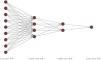
FCNN modelA fully connected neural network (FCNN) consists of a singular input layer, an output layer, and multiple hidden layers. Each neuron in a layer connects to every neuron in the preceding layer, with neurons distributed across these different layers. Fig. 2 illustrates an FCNN wherein the input layer is on the extreme left, the output layer, on the far right, and the hidden layers, between them. In both, the hidden and output layers, the neurons incorporate activation functions. These functions are crucial for converting the weighted sum of the inputs into nonlinear outputs, which are essential for the network’s predictive capabilities. The network architecture was designed for unidirectional signal flow with no feedback loops, allowing the signals to move seamlessly from the input to the output layer.

Let α(0)=x, and the fully connected neural network iteratively transmits information through Formulae (1) and (2):
Where W and brepresent the connection weights and biases of all layers in the network.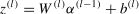

Our model design encompasses three key aspects:
- (a)
Overall Process Design: The experiment was conducted using Python 3.6. A fully connected neural network (FCNN) model was developed using the Google TensorFlow network. The Smote algorithm (Blagus & Lusa, 2013) was used to address the imbalance between positive and negative samples in the training set. The key hyper-parameters of the FCNN model were set as follows: epoch = 100, batchsize = 2000, learningrate = 0.005, and validationsplit = 0.2. The FCNN algorithm structure included (1) an input layer with the ‘relu’ activation function; (2) a hidden layer, also using ‘relu,’ with a dropout probability of 0.5, to periodically deactivate neurons, aiding in reducing overfitting; and (3) an output layer employing the ‘sigmoid’ activation function.
- (b)
Stock Sample Selection Strategy: To address the issue of limited historical data, which often restrict the number of training samples in machine learning for quantitative investment, we adopted two key strategies to ensure sufficient data for training deep learning models, particularly for medium- to long-term investment strategies, where the scarcity of independent sample points can affect model effectiveness. First, we included all stocks from the Shanghai and Shenzhen A-share markets (over 3000 stocks) to maximize the sample size. Second, we constructed the training dataset by selecting all A-share stocks following a historical "thousand-stock limit-down" event occurring at time t0. Each stock i was represented by its feature set Fi,t at time t, whereas the label yi,t was assigned, based on the stock's future price movement over the next 20 trading days (encoded as 1 if the stock rose and 0, otherwise). Here, i=1,2,3,⋯, approximately 3000, and t=t0+1,t0+2,⋯,t0+20. This approach ultimately generated a training set with over 60,000 samples, thereby meeting the data volume requirements for deep learning. Additionally, the test set was constructed, using daily stock data from the 20 trading days following the current crisis (denoted as t0current), to evaluate the model’s predictive capability. Specifically, the test set comprised feature sets Fi,t for each stock i (approximately 3000 stocks) over trading days t=t0current+1,t0current+2,⋯,t0current+20, resulting in a total of over 60,000 samples.
- (c)
Hidden Layers Design: The number and structure of hidden layers play a critical role in determining the performance of the FCNN model. Because financial research datasets tend to be much smaller than those used in image or natural language processing, where data volumes can reach hundreds of millions of samples, our training set of approximately 60,000 instances required a comparatively shallow network architecture. We found that three to six layers were sufficient for this sample size; adding more layers introduced a large number of parameters and increased the risk of overfitting. Consequently, this study focused on models with three, four, five, or six hidden layers. To ensure model robustness, each variant was tested 10 times and the averages were recorded. Additionally, while typical deep learning studies determine the optimal parameters for each network structure using criteria, such as information criteria or validation set performance, our objective was to validate our hypothesis across four thousand distinct stock limit-down crises. If we optimized the parameters separately for each crisis (e.g., selecting parameter A for 2018 data, parameter B for 2019 data, and parameter C for 2020 data), it would be unclear whether the observed differences were due to parameter optimization rather than the proposed approach, thereby introducing confounding factors. Consequently, we fixed specific parameters across all crisis events to facilitate a direct comparison. Generally, the number of neurons in hidden layers is designed to decrease with network depth, as reducing the neuron counts in deeper layers helps capture abstract, higher-level features that are more representative and discriminative, a strategy akin to data compression that enhances model performance in complex tasks. Given that our feature set comprises 128 variables, we started with 200 neurons in the first hidden layer for robustness. As shown in Table 2, the neurons in the hidden layers of FCNN follow a descending order that sufficiently reflects reasonable parameter design and reinforces our confidence in the conclusions.
Table 2.Hidden layers in the FCNN model.
The long short-term memory (LSTM) network, a variant of the recurrent neural network (RNN), was first introduced by Hochreiter and Schmidhuber (1997) and further refined in subsequent years by Gers and Schmidhuber (2000) and Gers, Schmidhuber and Cummins (2000). LSTM networks incorporate internal cell states and gating mechanisms, effectively addressing the issues of vanishing or exploding gradients, which are often encountered in traditional RNNs.
The LSTM cell is composed of forget gateft, input gateit, and output gateot. The mathematical principles and operational formulas are shown in Eqs. (3)–(8), respectively.
WhereWrepresents the corresponding weight matrix for each unit,brepresents the corresponding bias vector, and *denotes the Hadamard product of the matrices.


Fig. 3 illustrates a multilayer LSTM architecture consisting of m layers. As highlighted by Karpathy and Li (2017), the distinguishing feature of a multi-layer LSTM lies in its layered structure, where the input for the l-th layer is informed not only by its own processing, but also by output from the (l−1)-th layer. This design enables each successive layer to refine and build upon the information processed by the preceding layer, thereby enhancing the capacity of the network to learn intricate and abstract data patterns. The multilayered approach is particularly beneficial for complex tasks that require an in-depth understanding and recognition of long-term dependencies in sequential data.

This study’s LSTM model is methodically structured as follows:
- (a)
Overall Process Design: (1). Initial Dense Layer: The model begins with a fully connected (dense) layer, aimed at managing a large number of input variables. This layer is integral to feature-dimensionality reduction and is particularly beneficial for handling a multitude of variables. The reduced neuron count in this layer condenses the input data into principal components, thus simplifying the dataset for more efficient processing. (2). Stacked LSTM Layers: The core of the model comprises two LSTM layers strategically stacked to enhance the model’s capacity for learning. For most applications, stacking up to approximately four LSTM layers is sufficient. In the context of this study, considering the volume of available data, we stacked two layers. (3). Final Dense Layer: The final segment of the model was another dense layer designed for binary classification. Employing a sigmoid activation function, this layer translated the output of the model into a probability value ranging from zero to one. This probability reflects the likelihood of classifying input data into two predefined categories.
- (b)
Stock Sample Selection Strategy: The stock sample selection strategy for the LSTM model aligns closely with that of the FCNN model. In our training dataset covering 20 days, each day featured over 3000 stocks from the Shanghai and Shenzhen stock exchanges, resulting in over 6000 stock samples in both, the training and testing datasets.
- (c)
Key Parameters: The critical parameters of the model included the number of units in the first dense layer (unit1) and the number of hidden units in the subsequent second (unit2) and third (unit3) LSTM layers, as shown in Table 3. The model also considered time steps, incorporating both, a short-term lag of one week (five trading days) and a longer-term span of the following month (20 trading days). To verify the stability and reliability of the model, each parameter set was tested across ten separate experiments, and the average of these trials constituted the reported findings.
The confusion matrix categorizes the samples into four scenarios: true positives (TP), false positives (FP), true negatives (TN), and false negatives (FN), as shown in Table 4. Using the confusion matrix, common evaluation standards, such as accuracy, precision, recall, and F1-score, can be calculated.
Confusion matrix for classification results.
| Predicted Positive | Predicted Negative | |
|---|---|---|
| Actual Positive | True positives (TP) | False negatives (FN) |
| Actual Negative | False positives (FP) | True negatives (TN) |
Note: True positives (TP): number of samples correctly predicted as positive by the model. False negatives (FN): The number of positive samples incorrectly predicted as negative. False positives (FP): the number of negative samples incorrectly predicted as positive. True negatives (TN): the number of samples correctly predicted as negative by the model.
The three common evaluation metrics— Precision (P), Recall (R), and F1-Score— were defined and calculated as follows:
Precision (P):Precision measures the proportion of samples correctly predicted as positive among all samples predicted as positive,

Recall (R):Recall measures the proportion of samples correctly predicted as positive from all actual positive samples:

F1-Score:The F1-Score is the harmonic mean of Precision and Recall, and is used to measure the model's overall performance. It seeks a balance between Precision and Recall and is particularly useful for imbalanced classification problems:
Data description
Our research data were gathered exclusively from the SuperMind stock trading platform (https://quant.10jqka.com.cn/view/), a part of Tonghuashun’s quantitative investment platform, accessed on September 1, 2023. This platform offers a comprehensive analysis of 128 variables for all stocks in the Shanghai and Shenzhen A-share markets, encompassing both, technical and financial dimensions. Technical factors, used as momentum proxy variables, were divided into five categories: overbought/oversold indicators, volume-price indicators, trend indicators, energy indicators, and support/resistance indicators. Financial factors were classified as profitability, solvency, operational efficiency, growth potential, and valuation. Additionally, the significant influence of industry sectors was considered by including stock industry classification as a crucial variable.
Key aspects of our data preparation included the following:
- (a)
Stock Selection: We focused on stocks listed on the Shanghai and Shenzhen A-share markets as of January 1, 2020, and excluded any stocks that were IPOed after that date.
- (b)
Industry Classification: We used Tonghuashun’s industry classification from SuperMind, as of January 1, 2020, as a predictive sub-variable.
- (c)
Feature Set Compilation: The final training feature set was derived by intersecting the indicators from both, the training and test sets. First, factors with >80 % missing values were removed from the raw data. We then eliminated stock records containing missing data, resulting in a clean and robust training set.
- (d)
Data Standardization: We standardized the data by normalizing the indicators in the validation and test sets using the maximum and minimum values from the training set, as follows:
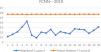
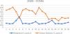
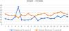
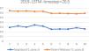
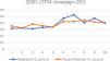
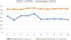
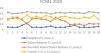
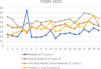
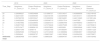
In China’s A-share market, the thousand stock limit-down events in 2018, 2019, 2020, and 2022 had unique causes: global turbulence and domestic slowdown in 2018, escalating trade frictions and tighter financing in 2019, the COVID-19 outbreak in 2020, and stricter macro-control policies in 2022. These events highlight the varied responses of the market to external shocks and internal pressures. Under these different conditions, we examined whether using post-crisis data from a previous crash ("distant relative data") as training data can improve one-month stock return predictions as compared to using data from the most recent crisis. To test this hypothesis, we designed multiple deep learning model architectures and parameter configurations by calculating Precision, Recall, and F1score for each scenario. We then conducted a Wilcoxon test with the null hypothesis H0:M0=M1 and alternative hypothesis H0:M0 Based on Table 1 and the FCNN model configuration, we trained the FCNN model, using two types of training data: "close neighbor" data (collected from near the crisis day) and "distant relative" data (obtained from a previous market crash). As detailed in Table 2, we experimented with three to six hidden layers and set five parameter groups for each configuration. Each parameter set was run ten times, and the average results were recorded. Tables 5–7 present the FCNN test set results for the 2019, 2020, and 2022 stock market crashes, and Figs. 4–6 illustrate the F1-scores across the various parameter groups. Results for the test set of 7 May 2019 and the subsequent 19 trading days. Results for the test set of 4 February 2020 and the subsequent 19 trading days. Results for the test set of 26 April 2022 and the subsequent 19 trading days. Table 5 shows that, for the 2019 crash, the FCNN model built using factors from Section 3.3, when trained with close neighbor data, achieved an average Precision of approximately 0.406, Recall of 0.187, and F1-score of 0.219. In contrast, when trained with distant relative data from the 2018 crash, the model produced an average Precision of about 0.403, Recall of 0.982, and F1-score of 0.571. The Wilcoxon test (p ≈ 0) confirms that training with distant relative data significantly improves performance. Fig. 4 visually demonstrates that using post-2018 data, rather than pre-2019 data, yields superior results, indicating that historical crisis data contain repeatable patterns. The 2019 crash was triggered by escalating trade frictions and tightened financing conditions, whereas the 2020 crisis occurred at the onset of the COVID-19 outbreak, driven by international uncertainty and liquidity shortages. Despite these differing backgrounds, we tested whether using post-2019 distant relative data as training data could enhance predictions of the 2020 crisis. As shown in Table 6, the model trained with close-neighbor data achieved an average Precision of 0.358, Recall of 0.066, and F1-score of 0.106, whereas using distant relative data improved these to a Precision of 0.381, Recall of 0.306, and F1-score of 0.312. The Wilcoxon test (p ≈ 0) confirms a significant improvement, and Fig. 5 further supports that distant relative data lead to better performance across most parameter groups. The 2022 crash, influenced by tightened macro-control policies and structural adjustments, presented another market environment. We evaluated whether training with post-2020 distant relative data could enhance predictions. As detailed in Table 7, the model trained with close neighbor data achieved an average Precision of 0.809, Recall of 0.202, and F1-score of 0.282, whereas training with distant relative data yielded improved averages of 0.872, 0.285, and F1-score 0.412. The Wilcoxon test (p < 0) confirms the superior performance of the distant relative data approach. Fig. 6 illustrates that, except for one parameter group, using distant relative data consistently outperforms the close neighbor data, further validating our findings of Sections 4.1.1 and 4.1.2. To further validate the findings of the FCNN model, we employed Long Short-Term Memory (LSTM) models, which are particularly effective in capturing temporal dependencies in stock pricing. This allowed us to compare the predictive performance of distant relative data with that of close-neighbor data for forecasting post-crisis stock returns. We evaluated the performance of the LSTM model using both, monthly (20 trading days) and weekly (5 trading days) time steps. Table 8 presents the LSTM model predictions for the 2019, 2020, and 2022 market crashes, and Figs. 7–9 illustrate the corresponding F1-scores. LSTM test set results following the 2019, 2020 and 2022 stock market crashes. As shown in Table 8, the Wilcoxon test yielded p-values close to 0 for the 2019 and 2022 crashes, indicating that using distant relative, rather than close neighbor, data significantly improves prediction performance. Specifically, the F1-scores for the A-share market post-crisis predictions, using close neighbor data, were approximately 0.288, 0.389, and 0.393 for 2019, 2020, and 2022, respectively. In contrast, using distant relative data yielded F1-scores of approximately 0.611, 0.386, and 0.630, respectively. These results suggest that, for the 2019 and 2022 crises, the LSTM model benefitted from historical crash data, which is consistent with the findings of the FCNN model. However, the 2020 results are less conclusive, likely because of the drastic market shift on February 3, 2020, which marked the first trading day after the COVID-19 outbreak, leading to a very different market environment compared to the pre-pandemic period. Overall, the performance of the LSTM model using distant relative data is superior or comparable to that using close neighbor data, reinforcing the robustness of our approach. Additionally, as shown in Tables 5, 6, 7 and 8, the average F1-scores for the FCNN model using distant relative data were 0.571, 0.312, and 0.412 for the 2019, 2020, and 2022 crises, respectively. By contrast shows that the LSTM model achieved higher average F1-scores of 0.611, 0.386, and 0.630 for the same periods. These findings underscore the advantage of the LSTM model in leveraging temporal memory to provide more accurate predictions than the FCNN model. In Section 4.1, we observed that the average F1 Scores for predicting post-crash stock returns using the FCNN model with distant relative data were 0.571 for 2019, 0.311 for 2020 and 0.411 for 2022. The F1 Scores for 2020 and 2022 were below 0.5, raising concerns regarding their practical utility. Deep learning models are particularly effective when trained on large datasets, and distant relative data can provide more comprehensive post-crash information, thereby improving prediction accuracy. To address this, we expanded the training approach for the 2020 and 2022 crises by incorporating two distant relative datasets instead of just one, as described in Section 4.1. Specifically, we used post-2019 and post-2018 data for the 2020 crisis, and post-2020 and post-2019 data for the 2022 crisis. The results showed significant improvements: for the 2020 crisis, the average F1 Score increased from 0.105 (using close neighbor data) to 0.311 (using a single distant relative dataset) and further rose to 0.627 (using two distant relative datasets). Similarly, for the 2022 crisis, the average F1 Score improved from 0.282 (close neighbor data) to 0.412 (single distant relative dataset) and reached 0.533 with two distant relative datasets, just above the 0.5 threshold, indicating practical value. These results demonstrate that training with multiple distant relative datasets significantly outperforms that with a single distant relative dataset, thus highlighting the importance of combining multiple historical crash events. Additionally, we explored the use of transfer learning by integrating close neighbor data with distant relative data. The model was first trained on two distant relative datasets and subsequently fine-tuned using close neighbor data. The results show that, for the 2020 crisis, the FCNN model, trained with transfer learning, achieved an average F1 Score of 0.448, and, for the 2022 crisis, a score of 0.395. Although transfer learning improved the performance compared to using a single distant relative dataset, it still did not surpass the accuracy of the model trained with both distant relative datasets. Figs. 10 and 11 further illustrate that using multiple distant relative datasets for training significantly improves prediction accuracy, with F1 Scores consistently above 0.5, across all 20 parameter sets. In contrast, the model trained using traditional close neighbor data performed the worst across all configurations. Overall, our findings suggest that, for post-crisis stock return predictions, training deep learning models with a combination of multiple distant relative datasets offer substantial practical value and enhance predictive performance. FCNN-2020 model’s F1 score with dual distant relative data and the transfer learning technique.


This study demonstrates the effectiveness of using historical crash data (referred to as "distant relative data") for forecasting post-crash stock returns in China’s A-share market. The results consistently show that utilizing distant relative data significantly improves predictive accuracy compared to traditional close neighbor data. This finding holds true for both, FCNN and LSTM models.
For the FCNN model, the average F1 scores for predicting post-crash stock returns using distant relative data are 0.571, 0.311, and 0.411 for the 2019, 2020, and 2022 crash periods, respectively. Notably, the F1 scores for the 2020 and 2022 crises were below 0.5, indicating limited practical utility. However, by incorporating data from two distant relative events, the F1 score for the 2020 crisis increased from 0.105 (using close neighbor data) to 0.311 (with a single distant relative dataset) and further to 0.627 (with two distant relative datasets). Similarly, for the 2022 crisis, the F1 score improved from 0.282 (using close neighbor data) to 0.533 (with two distant relative datasets), thus surpassing the threshold of 0.5, and providing a more practically useful model.
Additionally, the LSTM model outperformed the FCNN model, with F1 scores of 0.611, 0.386, and 0.630 for the 2019, 2020, and 2022 crashes, respectively, compared to the latter’s F1 scores of 0.571, 0.312, and 0.412, respectively. This demonstrates the advantage of LSTM in leveraging temporal dependencies to enhance the predictive performance.
Moreover, the use of transfer learning, which integrates close neighbor data with distant relative data, improved the model's performance, but did not surpass the accuracy of the model trained with both distant relative datasets. Specifically, transfer learning led to F1 scores of 0.448 and 0.395 for the 2020 and 2022 crises, respectively, which were lower than the F1 scores achieved by the model trained with two distant relative datasets (0.627 and 0.533, respectively).
Our findings indicate that training deep learning models with distant relative datasets significantly improves post-crisis stock return predictions, regardless of whether the model is based on the FCNN or LSTM architecture. Using a combination of multiple distant relative datasets, the trained FCNN model achieved F1-scores above 0.5 for both the 2020 and 2022 crises, demonstrating its practical applicability. Moreover, under the same settings, the LSTM models consistently outperformed the FCNN models, underscoring the advantage of LSTM in leveraging temporal dependencies.
A recent study by Ghasemieh and Kashef (2023) introduced robust deep learning models, such as the GAF-EWGAN stacking ensemble, for next-day price prediction during market crashes. Their study did not report explicit prediction accuracy; instead, it focused on evaluating post-crisis stock strategies, achieving an average annual return of 16.49 % across 20 stocks. In contrast, our approach analyzes the directional effects of stock returns across the entire A-share market (over 3000 stocks) following a crash.
In future research, one promising approach would be to build on our method-training models on historical post-crash data-and integrate it with advanced deep learning architectures, such as those proposed by Ghasemieh and Kashef (2023), to further enhance post-crisis stock return predictions. Another direction is to extend our methodology by employing statistical breakpoint techniques to detect structural shifts in market indices, such as the CSI 300. Once a new breakpoint is identified, the historical data following previous breakpoints can be used to train a deep learning model to forecast individual stock returns after the event. A significant challenge with this method is that accurate breakpoint detection requires data both, before and after an event, and timely identification remains a hurdle. Finally, our model was designed for emerging markets with frequent government intervention. Future research could also explore cross-market transfer learning, specifically by training a model on A-share data and testing its performance on Hong Kong stocks or other emerging markets.
CRediT authorship contribution statementWeiran Lin: Writing – review & editing, Writing – original draft, Supervision, Software, Methodology, Formal analysis, Data curation. Haijing Yu: Visualization, Software, Data curation. Liugen Wang: Supervision, Formal analysis, Conceptualization.
The author would like to thank the reviewers for their constructive comments. This research was supported by the Zhejiang Provincial Social Science Planning Special Project titled “Interpretation of the Spirit of the Third Plenary Session of the 20th CPC Central Committee and the Fifth Plenary Session of the 15th Zhejiang Provincial Committee.” Additionally, we gratefully acknowledge the advanced computing resources provided by the Supercomputing Center of Hangzhou City University.