


Spiking patterns observed at the output of lasers have been widely used to predict their dynamic behavior. The light output of a laser was associated with the coordinate of a particle moving in a potential well by Kleinman (1964). In this paper, this mechanical analogy is revisited so as to investigate a new approximation which might greatly simplify the relationships that determine the rate equations’ parameters. A ruby laser numerical example is presented to highlight the consistency of the proposed approximation near the equilibrium point.
Kleinman (1964) submitted a technical paper in which a mechanical analogy was used to analyze the behavior of spiking patterns observed at the output of lasers. An essential part of his analysis was based on the definition of a one dimensional potential field. In this paper, a new approximation for the potential field is introduced to obtain uncomplicated relationships for some quantities of experimental interest in the spiking pattern of a laser (e.g., interval between spikes and duration of the spikes).
The Statz–De Mars equations’ system has been widely used to model laser systems since its publication in 1960 (Aboites & Ramirez, 1989; Barrientos, Aboites, & Damzen, 1995; Statz & de Mars, 1960; Wilson & Aboites, 2013; Wilson, Aboites, Pisarchik, Pinto, & Taki, 2011; Wilson, Aboites, Pisarchik, Ruiz-Oliveras, & Taki, 2011). Originally designed to describe the oscillations in a maser, the model has since undergone many modifications to fit the description of laser systems (Aboites, Baldwin, Crofts, & Damzen, 1993; Aboites & Huicochea, 2010; Tang, Statz, & de Mars, 1963; Wilson, Aboites, Pisarchik, Pinto, & Barmenkov, 2011; Wilson & Huicochea, 2009).
The laser is a system consisting essentially of an optical cavity with very high quality factor (Q) in a few modes, low Q in all other modes, the laser medium containing the active atoms, and a pump, usually an intense light source, to excite the atoms into a broad band of excited states. The atoms decay from these states in an extremely short time by nonradioactive processes to one or more very sharp excited states, called the upper laser levels. The upper laser levels can decay radioactively to a sharp lower level, called the lower level laser, which may be the ground state. As long as we consider only a single mode of the cavity, the laser mode, and neglect all atomic populations except the upper laser level and the ground state, these equations may be written in the form:
where n is the population inversion, p the photon number, t0 (the pumping relaxation time) represents the characteristic time in the response of the population inversion n to the pump, tm (the mode time) represents the time for spontaneous emission into the laser mode, tp the photon lifetime in the laser mode of the cavity and s the source strength, the rate production of laser photons by spontaneous emission, the pumping light, or any other noise source in the cavity, or any signal applied to the cavity.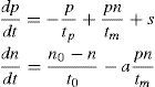
In order to simplify this equations’ system we used a well-known procedure to transform it into an dimensional one (Tarassov, 1981). We do so by defining the following parameters: ω=tp/t0, ξ=n0(tp/tm), σ=s(atpt0/tm), and the equation variables as: τ=t/tp, η=n(tp/tm) and ρ=p(at0/tm).
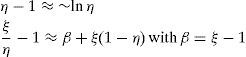
The adimensional Statz–De Mars equations’ system can be written as:
Here ρ represents the photons, η the inversion, and τ the time, while ω represents the pumping rate, ξ the limiting inversion towards which the pump is tending to drive the system, and σ the source. We shall assume that ω and ξ are constant. Typical values of the parameters for a ruby laser will be given in the discussion of the numerical example.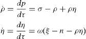
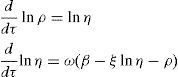
This system has to be adjusted so as to observe the spiking phenomena more clearly. For this reason, we assumed the spiking condition (ωξ≪1) and then analyzed the steady state solutions of (2) to obtain suitable approximations (Braun, 1992):
Thus, Eq. (2) may be transformed into:
Let us define the logarithmic light output as Ψ=ln(ρ/β). Then, the modified adimensional Eq. (4) that take into account the spiking are summarized as:
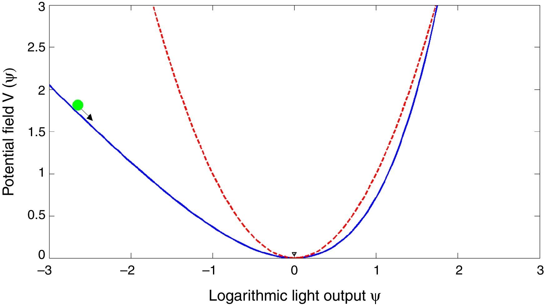
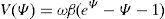
The discussion of (5) is facilitated with the aid of a mechanical analogy illustrated by Kleinman (1964). In which, Ψ would represent the coordinate of a particle of unit mass moving in a one dimensional potential field. The term ωξΨ would depict a dissipative resistive force that acts as a viscous medium, affecting the motion of the particle. The asymmetric potential (shown in Fig. 1) is written: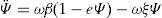
 moves in a potential field V(Ψ). The blue solid line represents the potential described by Kleinman (1964). The red dashed line represents the proposed parabolic approximation.")
Mechanical analogy in which a particle of unit mass with coordinate Ψ=ln(ρ/β) moves in a potential field V(Ψ). The blue solid line represents the potential described by Kleinman (1964). The red dashed line represents the proposed parabolic approximation.
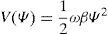
It was not obvious to us how much calculation could be reduced if the definition of the asymmetric potential field was simplified. For this reason, the exponential term in (6) was expanded using Taylor series with n=2 near the equilibrium point Ψ=0. The proposed parabolic potential (shown in Fig. 1) stands as follows:
What follows is a re-examination in Kleinman's analysis in order to provide simple relationships for some quantities of experimental interest in the spiking pattern of a laser.
Let us disregard the viscous force so that the total energy of the particle is conserved (E=V(Ψ+(1/2)Ψ˙2). The particle executes a periodic motion between extreme points Ψm<0 and ΨM>0 such that V(Ψm)=V(ΨM)=E. We then obtain a simple relation between the extreme points of motion in the spiking phase:

This result reveals the sinusoidal behavior of the spiking as τ→∞. It also gives a hint about when is suitable to use the following approximations. Before considering the damping, other quantities of experimental interest are taken into account which are characteristic of the periodic motion.
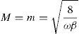
Let us denote by m the full width in time of the minimum measured between e times the minimum in the light output. Thus the duration of the minima is

Since the maximum and the minimum are so deeply related now, it is not surprising that the duration of the maxima has become
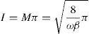
The most readily observed quantity in spiking experiments is the interval between spikes, which can be identified with the period of the quasi-periodic function I=ϕdΨ/Ψ where the integral is over one cycle. The interval may be obtained by analysing the time dependence of the logarithmic light output in the range Ψm≤Ψ≤Ψc and the range Ψc≤Ψ≤ΨM, where Ψc is a crossover point. Therefore,
We now return to the equation of motion (5) and consider the damping force – ωξΨ˙. The energy is no longer conserved because of the presence of damping and it decreases every cycle of motion until the particle settles down at its equilibrium position Ψ=0. The damping denoted by the increment ΔΨm or ΔΨM may be calculated with
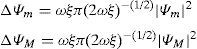
The damping increment for the maximums may be expressed more conveniently using (8) and (11):
3Ruby laser numerical example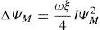
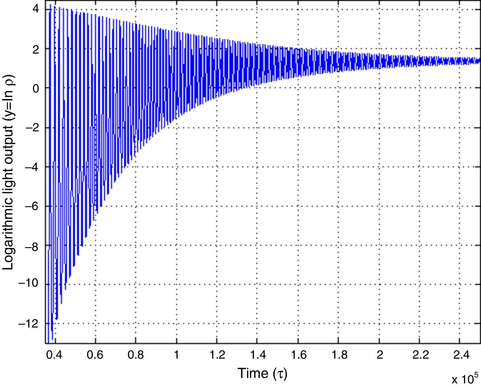
To find the solutions of the equations’ system (3) a MATLAB script was built using the typical values for a ruby laser ω=7.12×10⁻⁶, ξ=5, σ=2×10⁻⁹ and the initial conditions lnρ=lnσ, η=0 (Braun, 1992; Tarassov, 1981). We can see from Fig. 2 that the damping force reduces the oscillation as τ→∞. It is in this moment when the approximations carried out fit more accurately the laser dynamics and may be used to predict its behavior.
4Conclusions
We have presented a new approximation to the potential field in Kleinman's mechanical analogy which lead us to simple relationships for the interval between spikes and the duration of the spikes in laser spiking experiments. These relationships can be applied to decide whether a spiking pattern is consistent with the Statz–De Mars equations’ system (4).
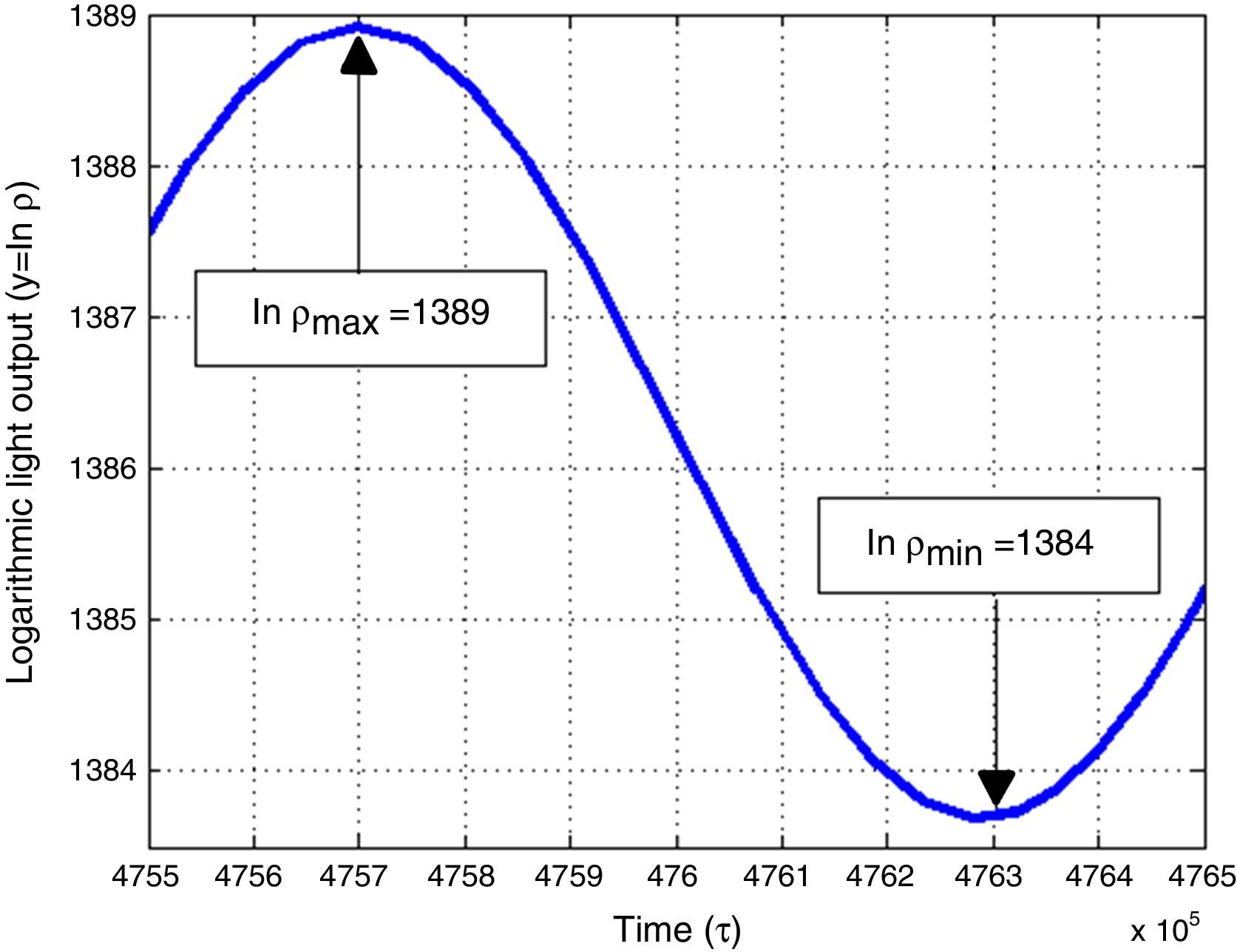
We also provided evidence of the consistency of (7) near the equilibrium point Ψ=0 through a ruby laser numerical example (Fig. 3). The results obtained in this work can be used in the future to find a method to calculate ω, ξ and σ just by analyzing the spiking patterns at the output of lasers.
Conflict of interest
The authors have no conflicts of interest to declare.
Peer Review under the responsibility of Universidad Nacional Autónoma de México.