


This paper uses System Dynamics modeling and process simulation to explore coordination in two logistic processes (procurement and production) of the supply chain of an ethanol plant. In that sense, three production scenarios are evaluated to identify: a) stock movement according to current inventory policies, and b) the critical variables affecting the coordination for these two processes. Since the main goal in the company is to meet customer demand, this research incorporates sales forecasting, and four performance indicators to evaluate the state of the processes: 1) average percentage of demand satisfaction, 2) maximum amount of ethanol in excess, 3) available ethanol at the end of the year, and 4) inventory costs. To model the case study, the change in production yield and specific constraints for the chain are considered. The simulation results show that System Dynamics modeling can be used to observe the effects of policies on inventory, and meeting the demand in a real system. It also can define the coordination for a supply chain and give information to improve it. The developed model uses STELLA® software to simulate the logistic processes and execute the evaluation employing the performance indicators.
Haciendo uso del modelado en Dinámica de Sistemas y simulación, se explora la coordinación de dos procesos logísticos (aprovisionamiento y producción) de la cadena de suministro de una alcoholera. En este sentido, la evaluación de tres escenarios de producción permite identificar: a) el movimiento del inventario de acuerdo a las políticas actuales de inventario, y b) las variables críticas que afectan la coordinación de estos dos procesos. Dado que el objetivo principal de la empresa es satisfacer la demanda del cliente, se incorpora un pronóstico de ventas, y cuatro indicadores de desempeño para evaluar el estado de los procesos: 1) el porcentaje promedio de la satisfacción de la demanda, 2) la cantidad máxima de etanol en exceso, 3) el etanol a disponer al finalizar el año, y 4) los costos de inventario. Para modelar el caso de estudio, se considera el cambio en el rendimiento de producción y las restricciones particulares de la cadena. Los resultados de la simulación muestran que la Dinámica de Sistemas puede utilizarse para observar los efectos de las políticas sobre el inventario, y la satisfacción de la demanda en un sistema real, igualmente, permite definir la coordinación para una cadena de suministro y proporcionar información para mejorarla. El modelo creado utiliza el software STELLA® para simular los procesos logísticos y para realizar la evaluación utilizando los indicadores de desempeño.
Any company that wishes to control the associated risk to corporative reputation and is willing to protect its value, starts ensuring an effective management of its supply chain [1], including all related activities to information, material, and funds flows from the stage of suppliers to the delivery of finished goods to end-users.
However, in order to administrate a supply chain and achieve the aim of maximizing the overall generated value [2], the decision makers need to consider the risk at every stage of the chain, especially when different actors make decisions only based on their own benefit [3]. All these logistic processes define the relationship among risk, cost, and supply chain surplus of a company [4][5].
In this paper, a case study regarding an ethanol plant shows a supply chain with two independent suppliers (one for each of the two main raw materials: molasses and grain sorghum). The plant only supplies one product (ethanol), and counts with a demand driven production system. Hence, using System Dynamics modelling, the supply chain is simulated in order to assess the effects of three production plans to meet the forecasted demand, and understand the kind of impact on inventory policies and the suppliers responsiveness.
The structure of this paper is as follows: a brief literature review is provided in Section 2; and the case study is addressed in Section 3. The model to evaluate the production plans is introduced in Section 4; simulation results and analysis are provided in Section 5. Finally, Section 6 discusses practical and derived managerial insights from the simulation and statistical results.
2Literature reviewThis section describes the main concepts of System Dynamics modeling, and presents several related works concerning the application of this approach to design supply chains.
2.1System DynamicsSystem Dynamics (SD) is a method to enhance learning in complex systems. It deals with feedback loops, variables, levels, and delays that affect the system's behavior over time [6].
Since SD approach is intended to avoid policy resistance and finding high leverage policies [7], a causal loop diagram (CLD) is an important tool to represent the feedback structure of a system, shows the involved elements in reality, and let us know and understand its behavior.
Even the best conceptual model can only be tested and improved by relying on the learning feedback provided through the real world. However this feedback is very slow and often rendered ineffectively by dynamic complexity, time delays, defensive reactions, and costs of experimentation, among others. Under this complexity and constraints, simulation is a practical way to test a model. Additionally, when experimentation in real systems is not possible, simulation becomes the only way to discover how a complex system works. In this sense, Cedillo-Campos and Sánchez-Ramirez [8] suggested four phases to develop System Dynamics models: conceptualization, formulation, evaluation, and implementation.
2.2System Dynamics and Supply ChainSystem Dynamics is useful to observe a set of interacting elements where each of them has a performance based on a common goal. This approach has been extensively studied to understand and examine the behavior of supply chains. Discrete event simulation is also a widely used tool; nevertheless, according to Tako et al., it has no clear advantage over SD [9].
For the first issue, Nam et al. [10] suggested a knowledge-management method to improve organizational performance. Potter and Lalwani [11] aimed at quantifying the impact of demand amplification on transport performance. Springer and Kim [12] used three distinct supply chain volatility metrics to compare the ability of two alternative pipeline inventory management policies in order to respond to a demand shock. Huang et al. [13] contributed to the literature by providing a better understanding of the impacts of supply disruptions on the system performance, and shedding insights into the value of a backup supply. Maheut et al. [14] evaluated transport policies at an automotive industry without affecting the supply chain performance.
For the second issue, Shin and Lee [15] used QFD and SD approach to simulate and evaluate key policies related to the improvement of key indicators. Li et al. [16] used SD to simulate the management process of the power grid-engineering project. Bouloiza et al. [17] used SD to evaluate unusual scenarios in order to improve safety of the industrial system and implement managerial tools involving organizational, technical, and human factors. Stave [18] illustrated the process of building a SD model in a case study, which evaluates water management.
Anyhow, when the supply chain is defined, different studies consider demand as an important feature. Thus, Suryania et al. [19] developed a SD model to forecast air passenger demand and to evaluate some policy scenarios related to runway and passenger terminal capacity expansion to meet the future demand. Qia and Changa [20] designed a SD model for the prediction of municipal water demand.
It is important to emphasize that SD is widely used to design supply chains. However, this approach is also employed in different fields and for different purposes, as it is demonstrated by Hsu [21], where different policies are evaluated in order to achieve the goal of reducing the emission of carbon dioxide, or by Rehana et al. [22], where the approach is proposed to help water utilities meet the requirements of new financial regulations. For Wang [23], the SD approach is presented based on the cause-and-effect analysis and feedback loop structures to restrict the total number of vehicles in order to improve the sustainability of transportation system.
3Case study: Ethanol plantThree main logistics processes compose the structure of a supply chain: procurement, production, and distribution [24]. The case study proposed in this paper addresses the supply of feedstock (procurement) and the production processes in an ethanol plant located in Veracruz, Mexico.
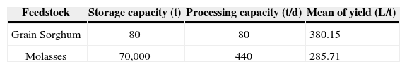
This company uses two main raw materials to produce ethanol: grain sorghum and molasses. In the case of grain sorghum, the company has a main supplier with a capacity defined by the soil yield and the harvest seasons. On the other hand, the milling and refining of sugarcane in surrounding mills determines the availability of molasses. The supply chain of this company is shown in Figure 1.

Since the company wishes to meet the customer demand, it needs a tool to determine whether its production plan is coordinated with the stages of supply and production stages of its supply chain. In order to achieve this, the company must ensure two situations: 1) yields to produce ethanol in the right quantity for their customers, based on current operating conditions and the type of feedstock, and 2) availability of enough feedstock to satisfy the production plan based on its current inventory policies and responsiveness of its suppliers.
An important situation to highlight is the fact that the company has three cycles of production per year, followed by 15 days of equipment maintenance.
Data about capacity, yield, and storage constraints in the company is shown in Table 1.
4MethodologyThis section introduces the parameters and the CLD for the case study, and presents the simulation model using STELLA® software.
4.1Causal loop diagramsA causal loop diagram consists of variables connected by arrows denoting the causal influences among the variables. For each causal-loop a polarity is assigned and may be positive or negative. A positive link means that if the cause increases, the effect also increases; or, if the cause decreases, then the effect decreases as well. A negative link follows an inverse principle. Thus, if the cause increases, then the effect decreases, or, if the cause decreases, then the effect increases [7].
It is important to underline that link polarities describe the structure of the system, but not necessarily the actual behavior of the variables. The important feedback loops are also identified in the diagram. Every loop is highlighted with a label showing whether the loop is a negative (also known as balancing) or positive (also known as reinforcing) feedback.
The developed CLD to model the system is presented in Figure 2. In the diagram important variables from the case study are identified, which help develop the stock and flow diagram in the simulation software. The feedback loops have a loop identifier.
- •
In Loop B1, if the molasses stock of the supplier increases, then the procurement based on meeting order quantity also increases. Moreover, an increase in meeting order quantity means a decrease in the molasses stock of the supplier.
- •
In Loop B2, a decrease in grain stock will decrease the grain procurement, and if this meeting order quantity increases, the grain stock of the supplier decreases.
- •
In Loop B3 and Loop B4, if the ethanol production increases, the molasses and the grain stock decrease. However, if one of these stocks increases, the ethanol production will increase in the same way.

In order to explore the coordination process of procurement and production, current policies in the company were studied to have enough information to feed the simulation model.
1)ProcurementThe procurement stage involves several actions. Among the most important are: supplier's selection, definition of the order quantity, the purchase frequency of raw material, and the inventory control. Thus, it is necessary to consider information about the suppliers in order to improve coordination of procurement and production, and eventually, achieve an effective overall coordination in the supply chain.
For grain sorghum, at 2014, it is considered that the supplier will have a 10,000 tons (t) safety stock, in addition to 8,982 hectares (ha) available for grain crop, minus 22.55% historically affected after agricultural cycle. The agricultural cycle begins in May and finishes in June with a regrowth from November to December. The soil yield for this crop is estimated at 2.7504 t/ha, and below 50% during regrowth. Moreover, for the start of 2014 the company will have a 60 tons stock of grain. The inventory policy currently applied at the company consists in a reorder point (ROP) as in (Eq. 1) with a lead time (LT) of 1 day, a service level (SL) of 99%, 2 backup days (BD) to calculate the safety inventory (IS) according to (2), and an order quantity (Q) based on the replenishment of the storage capacity.

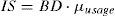
In (Eq. 1) and (Eq. 2), ¿usage and ¿usage respectively represent the mean and the standard deviation for the use of feedstock.
The total cost (TC) function for the grain sorghum, including purchase, ordering, and holding cost is shown in (Eq. 3).

In (Eq. 3), n represents the number of grain sorghum orders by year, G stands for the average grain sorghum quantity in stock, and Cgrain is the cost of the grain sorghum as a function of time.
Now, in early 2014 the company estimates a molasses stock of 15,000 tonnes, and its inventory policy consists of a reorder point as in (Eq. 1), with a lead time of 7 day, a service level of 99%, and 30 backup days to calculate the safety inventory as in (Eq. 2). Additionally, the order quantity is fixed at 30,000 tonnes. Nevertheless, the company can only receive a maximum of 32 freights of 25 tonnes per day.
The total cost (TC) function for the molasses, including purchase, ordering, and holding cost is shown in (Eq. 4).

In (Eq. 4), w represents the amount of molasses orders per year, M represents the average molasses quantity in stock, and Cmolasses is the cost of the molasses.
The constant values in (Eq. 3) and (Eq. 4) are based on a cost analysis with the current conditions in the company as Garcia suggests [25]. It also considers the cost of raw materials and the holding cost that includes the effective spaces in the warehouses, and the different investments for their maintaining, as well as the money invested in purchasing department.
2)ProductionThis step includes all unit operations and processes carried out in order to obtain a finished good.
It is important to define production as a process closely linked to the ability of the company to have a system, which may respond to the needs of the customer.
Ethanol production in the company is of semi-continuous type, where each batch of raw material is daily introduced into the system, and each load of product is obtained at the end of the day.
Therefore, for the grain sorghum case, the errors obtained with the average and historical yield were fit to a distribution. Thus, an accurate yield in the company by using grain sorghum as feedstock could be known through the relation suggested in (Eq. 5), which includes a transformation of Johnson.

In (Eq. 5), eg is the error in the yield using grain sorghum and, according to a statistical analysis with historical data, it is normally distributed with a mean equal to −0.08840, and a standard deviation equal to 0.994282.
For the case of molasses, a regression analysis was computed by using the historical yield. Then, the errors concerning the historical yield and the regression were fit to a distribution. Therefore, an accurate yield in the company by using molasses could be known by the relation suggested in (Eq. 6).

In (Eq. 6), em is the error in the yield using molasses, which is normally distributed with a mean equal to 0, and a standard deviation equal to 2.31933. Also, d represents the day in a production cycle. It is important to underline that there are three production cycles in a year; each one is followed by a period of 15 days of equipment maintenance.
In order to manage production it is also necessary to calculate an estimate of future demand. Therefore, a forecasting analysis was developed considering the monthly ethanol demand during 2012.
Three hypothesis tests with a level of significance of 5% were used to evaluate randomness, autocorrelation, and trend; i.e. stationarity. These tests were performed as part of the methodology suggested by Farnum and Stanton [26]; however, when the number of data is small as is in this case, Hanke and Wichern [27] suggest using a stationary model, because this explains the behavior of sales better than a sophisticate model.
In any case, the tests confirmed the assumption of Hanke and Wichern. Consequently, the evaluation of forecasting error, among the evaluated stationary models, placed the moving average with length 8 as the best. Then, the monthly sales were expected to be uniformly distributed in the forecast interval of 95% from 2,252,342L to 3,113,847L.
The forecasted demand is proportionally divided by the number of days of the corresponding month. Thus, the demand is assumed as uniform and the summation achieves the forecasted value at the end of month.
3)Performance indicator:In order to define the coordination of the procurement and the production, four performance indicators were suggested. These are the average percentage of demand satisfaction, the maximum amount of ethanol in excess during the year, the available ethanol at the start of next year, and the inventory costs.
The average percentage of demand satisfaction ( APS) is presented in (Eq. 7).

In (Eq. 7), j represents the number of days in the year, s represents the effective sale, and D represents the ethanol demand according the forecasting.
The maximum amount of ethanol in excess (MEE) during the year is evaluated using a conditional: if the ethanol stock is over the actual capacity (2,080,000L), then the maximum excess is selected. This function is represented in (Eq. 8), where ES represents the amount of ethanol in the stock, while the subscripted i represents any day of the year.
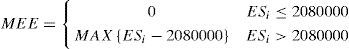
The amount of ethanol available at the beginning of next year ( ESj) will simply be the amount in stock left at the end of this year. This is considered as a performance indicator, because the initial stock for 2014 is estimated at 1,000,000L. Hence, the amount of ethanol in stock for early 2015 should be ensured in the same way.
Finally, the inventory costs are evaluated as in (Eq. 3) and (Eq. 4), where the average quantity in stock of feedstock is dynamically computed as an arithmetic mean by using the simulation model.
4)Simulation modelBy using the CLD and the parameters explained above, the stock and flow diagram were built on the simulation software. A length from 1 to 365 days (representing 2014) and one day were used as simulation units. This CLD is used by evaluation a validation the model [28, 29].
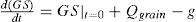
Equations (Eq. 9), (Eq. 10), (Eq. 11), and (Eq. 12) describe the behavior of the subsystems composing the developed model. In these subsystems ES represents the ethanol stock, GS the grain sorghum stock, GSS the grain sorghum stock in the supplier, MS the molasses stock, g stands for the amount of grain to be processed, m for, the amount of molasses to be processed, ygrain and ymoasses represent the yields in the production of ethanol from grain or molasses, s the effective daily ethanol sales, Qgrain and Qmolasses the order quantities of feedstock, and finally, r represents the reception of molasses in the company.
5Results and discussion


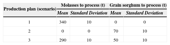
The results presented below are based on testing three production plans, which appear in Table 2. Since the model uses uniform and normal distributions to define parameters, such as forecasted demand, yield and amount of feedstock to process, 10 pilot runs with each scenario (see Table II) were executed to obtain the optimal number of runs according to (Eq. 13) suggested by Law and Kelton [30].
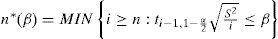
In (13), n*( ¿) represents the optimal number of runs, n stands for the number of pilot runs, and ¿ represents an absolute error for the mean estimator based on the standard deviation (s2) of the pilot runs sample and the Student t distribution.
For the first scenario, with 95% confidence, the APS is 98.5% (±1%), the MEE is 139,257.09L (±45,000L), the ESj is 316,627.94L (±75,000L), the TCgrain is 17,529.32 MXN, and the TC, 268,077,306.30 MXN (±2,500MXN).
Figure 3 shows the ethanol stock movement and the daily percentage of demand satisfaction for the first scenario. The amount of ethanol available can meet the demand during the whole year, except from day 242 to day 245 of 2014, which is the period when there is not enough ethanol to satisfy the demand.

The shortage cannot be due to a lack of coordination with the feedstock supply. Indeed, under this condition, the molasses stock in the company does not suffer any shortage or there is an overstock of it, as shown in Figure 4. In that sense, during the second period for equipment maintenance, the daily percentage of demand satisfaction falls to zero due to that shortage, and rises again when the third production cycle of the year starts. Thus, considering these circumstances, this production plan can be more effective if the period for equipment maintenance is reduced while it is possible.

In the second scenario, with 95% confidence, the APS is 20.18% (±0.25%), the MEE is 0L, the ESj is 0L, the TCgrain is 56,351,872.92 MXN (±136,000MXN), and the TCmolasses is 3,023,478.97 MXN.
Figure 5 shows if the company uses a plan where grain sorghum is the only feedstock to be processed. As an average the daily percentage of demand satisfaction will not rise over 20.18%. The shortage of ethanol is caused by two factors. The first cause is that the amount of grain is not enough to produce the amount of ethanol demanded. The second cause is a disruption of feedstock supply due to the current inventory policy. However, the grain sorghum supplier has no problems of shortage, as shown in Figure 6. This demonstrates a proper coordination in the procurement process but not in the feedstock supply to production.


The lack of coordination of the inventory policy and the production plan (according the second scenario) is shown in Figure 7, which reveals a grain sorghum shortage during the production cycles of the year, and an overstock during the periods for equipment maintenance (time when the daily percentage of demand satisfaction falls to zero, as shown in Figure 5). This situation can be improved by changing the current storage capacity, but does not imply an increase of the APS.

Finally, for the third scenario, with 95% confidence, the APS is 98.54% (±1%), the MEE is 153,423.27L (±25,000L), the ESj is 240,090.05L (±94,000L), the TCgrain is 48,391,245.19 MXN (±136,000MXN), and the TCmoiasses is 201,500,248 MXN (±2,500MXN).
Figure 8 shows the ethanol stock and the daily percentage of demand satisfaction for the third scenario. In this scenario the ethanol stock is correctly coordinated, since there is no shortage or overstock, and the daily percentage of demand satisfaction is totally achieved. However, considering the performance indicators, there are no important differences between this third plan and the first one.

For the fourth scenario, with 95% confidence, the APS is equal to 97.26% (±1%), the MEE to 94,777.81L (±45,000L), the ESj to 84,371.78L (±75,000L), and the TCmolasses is equal to 268,103,361.50 MXN (±2,500MXN). On the other hand, for the fifth scenario with 95% confidence, the APS is equal to 99.48% (±1%), the MEE to 123,035.66L (±45,000L), the ESj to 453,356.75L (±75,000L), and the TCmolasses is equal to 267,993,078 MXN (±2,500MXN). In both scenarios, the TCgrain has no changes with regard to the first scenario.
6Conclusions and future workThrough the use of this simulation model it can be proved whether a certain plan of production can satisfy the customer's demand, and also if the procurement and production stages are properly coordinated under current operational conditions.
As shown in Section 5, by performing the second plan for 2014, where molasses are not processed, the company would achieve a low level of demand satisfaction. When the production plans include the process of molasses or a mixture of raw materials (molasses and grain sorghum), the demand can be met in 98.5% (±1%), mostly due to the coordination in the supply of molasses. However, the first scenario has a higher cost associated to inventory.
Nevertheless, when the time for equipment maintenance changes for the first scenario, an increase in that parameter means a decrease in the meeting demand and vice versa, and thus, the storage capacity becomes a critical variable.
The identified critical variables in the studied model are: the storage capacity of grain sorghum – since a small capacity limits the daily consumption of production; the storage capacity of ethanol – because it establishes the limit to the ethanol production; the amount of raw material that goes into the process – as ethanol production depends on these quantities; the time spent on equipment maintenance – because if the period for maintenance increases, the shortage increases as well; and the order quantity for grain sorghum, because this amount can generate overstock or shortage.
As a consequence of the relationships established among the variables and the constraints of the system, the model allows the company to evaluate different conditions and figure out the performance indicator and the results. Both aspects statistically supported.
As future work, it is recommended to incorporate a mathematical algorithm into the model, or using a special technique, such as genetic algorithms, that is able to take this simulation to the evolutionary computing. Another recommendation is to analyze other stages in the supply chain, such as the distribution and service stages.
The authors wish to thank the National Council for Science and Technology in Mexico (CONACyT) and the Asociación Mexicana de Cultura, A.C, This work was additionally supported by the General Department of Technological Higher Education (DGEST) and the Secretariat of Public Education in Mexico (SEP) through PROMEP.