


Bayesian Belief Network (BBN) is an appealing classification model for learning causal and noncausal dependencies among a set of query variables. It is a challenging task to learning BBN structure from observational data because of pool of large number of candidate network structures. In this study, we have addressed the issue of goodness of data fitting versus model complexity. While doing so, we have proposed discriminant function which is non-parametric, free of implicit assumptions but delivering better classification accuracy in structure learning. The contribution in this study is twofold, first contribution (discriminant function) is in BBN structure learning and second contribution is for Decision Stump classifier. While designing the novel discriminant function, we analyzed the underlying relationship between the characteristics of data and accuracy of decision stump classifier. We introduced a meta characteristic measure AMfDS (herein known as Affinity Metric for Decision Stump) which is quite useful in prediction of classification accuracy of Decision Stump. AMfDS requires a single scan of the dataset.
Bayesian Belief Network (BBN) is a notable formalism in structure learning. It is based on joint probability distribution in which every question is submitted to the network in a probabilistic mode and the user can receive the answer with a certain confidence level. A BBN in short is composed of three components. < G, ¿, D > in which G is a Directed Acyclic Graph (DAG). As from the graph theory we know that each graph is composed of two elements and same is true for G such that G=(V, E). The DAG technically reprents the quality of a model rendered by the structure learning procedure because it is comprised of all of the dependent and independent nodes. Infact the absence of certain arcs realize the conditional independence of the nodes. Moreover G posses a probability ¿ which is a quantitative component of structure learning, an indicative of implicit degree of association between the random variables. The vertices in G usually denotes the random variables such that X=(X¿)¿∈V and ¿ represents the joint probability distribution of X with ¿(X)=¿¿∈V¿(X¿ | Xpa(¿)) where ¿(X¿ | Xpa(¿)) shows a conditional distribution and pa(¿)is the set of parents of ¿.
BBN has proven its usefullness in the diversified domains such as bioinformatics, natural language processing, robotics, forecasting and many more [1]–[3]. The popularity of BBN stems from its generatlity in formalis and amenable visualization because it enables the viewers to render any expert based modification. The process of structure learning is comprised of two major components excluding setting of external parametres. However both of these steps are layered in onion style structure. The first component is a traversing algorithm which takes input variables and formulates a structure in shape of a Directed Acyclic Grapg (DAG).This structure is handed over to the second component. The second component is a discriminant function which evaluates the goodness of the structure under inspection. The discriminant function in BBN captures the assumption during learning phase that every query variable is independent from the rest of the query variables, given the state of the class variable. The goodness of the structure is produced in form of a numeric value. The search algorithm caters for the comparison of last value and current value produced by the discriminant function and marks one of them as the latest posible structure. In a simple brute force searching mechanism, every candidate of BBN structure is passed to evaluate its discriminant function after which the BBN with highest discriminant function is chosen.
Although brute force provides a gold standard, however it is restricted to dataset with only a very small number of features as otherwise generating a score (output of discriminant function) for each possible candidate is NP hard with the increasing count of nodes in structures. A solution to tackle this NP-hard issue is to restrict the number of potential candidates for parent nodes and employing a heuristic searching algorithm such as greedy algorithm [4], [5]. In the greedy search algorithm, the search is started from a specific structure which initially takes the input variables in a predefined order. The obtained structure is analyzed by the discriminant function which results in adding, deleting or reversing the direction of the arc between two nodes. The ordering of the query nodes is characterized by the prior knowledge or by means of sophisticated techniques such as defined by [6]. The search continues to the adjacent structure reaching to the maximum value of a score if this value is greater as compared to the current structure. This procedure, which is known as hill-climbing search halts when culminating to a local maxima. One way of escaping local maxima is to employ greedy search. While employing greedy search, random perturbation of the structure is the way through which local maximum can be avoid off. Apart from this approach, there are alternate approaches escaping of local maxima problem. These include simulated annealing introduced by [7], [8] and best-first search [4]. In other words, if one describes the procedure of K2 [9] in simple words then pursuit of an optimal structure is more or less equivalent to selecting the best set of parents for every variable but avoiding any circular dependency. This is the basic concept behind the K2 algorithm.
However, it is an interesting question whether classification accuracy or error rate is sufficient enough for introduction of a new data model learner. There are situations when large number of variables degrades the performance of the learnt network by increasing the model complexity. This issue has motivated us to investigate the behavior of model complexity for various discriminant functions.
This study discusses the issue of formally defining ‘effective number of parameters’ in a BBN learnt structure which is assumed to be provided by a sampling distribution and a prior distribution for the parameters. The problem of identifying the effective number of parameters takes place in the derivation of information criteria for model comparison; where notion of model comparison refers to trade off ‘goodness of data fitting’ towards ‘model complexity’.
We call our algorithm Non Parametric Factorized Likelihood Discriminant Function (NPFLDF). The proposed discriminant function is designed to increase the prediction accuracy of the BBN model by integrating mutual information of query variable and class variable. We performed a large-scale comparison with other similar discrattempt functions on 39 standard benchma UCI datasets. The experimental results on a large number of UCI datasets published on the main web site of Weka platform show that NPFLDF significantly outperforms its peer discriminant function in model complexity while showing almost same or better classification accuracy.
2Model ComplexityThe BBN model complexity has been conceptualized in many ways. One simple concept is the frequentist approach of dependent and independent query variables. Another approach is related to the joint distribution of the observed query variables and the random parameters (varies from one discriminant function to another). However we argued for the second approach as in case if the distinct states are few or features are binary in nature then frequentist approach becomes the lonely dominant criteria for explaining the model complexity. Keeping in view of this assumption we shall introduce the mathematical formulation for model complexity along this line.
Lemma 1. The maximum links in a directed acycle graph can be termed as the model complexity. The problem of model complexity is a frequentistic solution.
Proof. Let N be the total number of nodes in a DAG excluding class attribute, then problem of finding the maximum possible nodes is equivalent to the ‘How to sum the integers from 1 to N’ problem and can be expressed as.

Let P be the constraint of maximum links a node can have in terms of its parent nodes. We can divide all of the links in two sets, one set ¿cn belongs to the arcs realized by the nodes with constraint and the second set ¿ot represents all other arcs. We express it as:

Certainly, if the constraint is in its first value (level); that is each node can have maximum one and only one arc then the BBN model will be a simple BBN structure. A higher value of constraint will lead towards more arcs in the second set. Let P denotes the constraint such that each node can have maximum P nodes as its parent nodes with whom the node is independent of, then the second set ¿cn can further be divided into two sub sets ¿≥Pcn and ¿

The count of the maximum links for the first subset ¿≥Pcn can be defined as:

The second subset comprised of the links in which first node can have maximum one parent node, second node can have maximum two parent nodes, third node can have maximum three parent node. If we continue this pattern then last node can have maximum P-1 parent nodes such that.

Notice that if value of P is one, then the above subset is an empty subset. Now based on the above last three equations, we can re write the equation of set of links with constraint such as:

From the above equation, we can derive a simple mathematical formula such as:

Where P is the constraint on count of máximum parents, a node can have and N is the total number of non class features or query variables. The equation 5 is a frequentistic representation of model complexity. At this point it is quite easy to calaculate the model complexity in percentage as below.

The above equation is quite useful for calaculating the numeric value of the model complexity in this study. The detailed result will be discussed in empirical validation section.
3Related workThere are two essential properties associated with any discriminant function to optimize the structural learning [10]. The first property is the ability of any discriminant function to balance the accuracy of a structure keeping in view of the structure complexity. The second property is computational tractability of any discriminant function (metric). Bayes [9], BDeu [11], AIC [12], Entropy [13] and MDL [14], [15] and fCLL [16] have been reported to satisfy these characteristics. Among these discriminant functions, AIC, BDeu and MDL are based on Log Likelihood (LL) as given below:
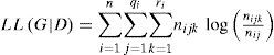
Where G denotes directed acyclic graph given dataset D. Other three counters include n, qi and ri indicate number of cases, number of distinct states of a query variable and number of distinct states of parent variable of a ith query variable. The log likelihood tends to promote its value as the number of features increases. The phenomenon occurs because addition of every arc is prone to pay contribution in the resultant log likelihood of final structure. This process can be controlled somewhat by means of introduction of penalty factor or otherwise restricting the number of parents for every node in the graph. The mathematical detail of the discriminant functions in this study are as follow.
3.1AICAkaike Information Criterion (AIC) originally defined by Akaike [12] is defined mathematically:

In the equation 10, K denotes the number of parameters in the given model. However, [17] decompose AIC into a discriminant function which can be used in BBN. AIC is established on the asymptotic behavior of learnt models and quite suitable for large datasets. Its mathematical equation has been transformed into.

Where |B| is length of network, number of parameters for each variable.
3.2BayesWe earlier mentioned that Cooper and Herskovits introduced an algorithm K2 in which greedy search was employed while a discriminant function of Bayes was used [9]. It was described that the structure with highest value of Bayes metric was considered the best representative of the underlying dataset. It motivates us to describe Bayes metric formally expressing in mathematical notations.
Let there is a sequence of n instances such that zn=d1d2d3.....dn the Bayes discriminant function of structure g ∈ G can be formulated in form of the equation.
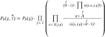
Where Pb (g) is the prior probability of full network g ∈ G.The prior probability can be omitted in the computation. The notation j ∈ J={1,….,N} is the count of the variable of the network g, and s ∈ S(j,g) is the counting of the set from all sets of values obtained from the parents of the jth node variable. The expansion of the denominator factor can be expressed mathematically as below.

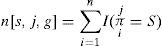
Where ¿j=¿j, the function I(E)=1 given E is true, and I(E)=0 if E is false. The K2 learning algorithm uses Bayes as its core function in its each iteration enumerating all potential candidate graphical structure. The outcome of this enumeration is an optimal learnt structure which is stored in g*. This optimal structure possess highest value of Pb(g,zn) such that ∀g ∈ G−g0, ifPb(g,zn)>Pb(g*,zn), then g* ← g.
The above equation is required to be decomposed simply into a computational model; otherwise this theoretical model requires a very large number of computations involving factorial. It means score value for a network g can be enumerated as the sum of scores for the individual query variables and the score for a variable is calculated based on that variable alone and its parents.
The approach in the “discriminant function inspired learning” performs a search through the space of potential structures. These include Bayes, BDeu, AIC, Entropy and MDL, all of which measures the fitness of each structure. The structure with the highest fitness score is finally chosen at the end of the search. It has been pointed out that Bayes often results in overly simplistic models requiring large populations in order to learn a model which holds the capability to capture all necessary dependencies [18]. On the other hand, BDeu tends to generate an overly complex network due to the existence of noises. Consequently, an additional parameter is added to specify the maximum order of interactions between nodes and to quit structure learning prematurely [19]. As noted in another research that the choice of the upper bound given the network complexity strongly affects the performance of BOA. However, the proper bound value is not always available for black box optimization [20].
Nielsen and Jensen in 2009 discussed two important characteristics for discriminant function used in the belief network [10]. The first characteristic is the ability of any score to put the accuracy of a structure in-equilibrium in context of complexity of structure. The second characteristic is its computational tractability. Bayes has been reported to satisfy both of the above mentioned characteristics. Bayes denotes the measurement of how well the data can be fitted in the optimized model. The decomposition of Bayesian Information Criterion [21] can be preceded as below:

Where ¿¿ is an estimation of the maximum likelihood parameters given the underlying structure S. It was pointed out that in case of completion of the database, Bayesian Information Criterion [21] is reducible into problem of determination of frequency counting [10] as given below:
where Nijk indicates the counts of dataset cases with node Xi in its kth configuration and parents ¿(Xi) in jth configuration, qi denotes the number of configurations over the parents for node Xi in space S and ri indicates the states of node Xi.3.3BDeu
Another scoring measure which depends only on equivalent sample size N′ is Bayesian Dirichlet for likelihood-equivalence for uniform joint distribution (BDeu) introduced by [11]. Later on, researchers have provided and discussed its decomposition as below in mathematical form [16]:
3.4MDL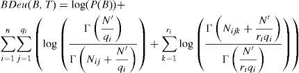
Minimum Description Length (MDL) introduced by [14] initially and then refined by [22], and [15]. It is mostly suitable to complex Bayesian network. We shall formally define it as below. Let sequence xn=d1d2d3.....dn of n number of instances, the MDL of a network g ∈ G can be enumerated as below.
L(g,xn)=H(g,xn)+k(g)2⋅log(n) Where the function k(g) represents the independent conditional probabilities in the network. H(g,xn) is entropy of structure with respect to the variable xn which can be expanded into the following notation.

Given the jth node variable, the value of MDL can be enumerated as below:
is the count of independent conditional probabilities of jth variable. This value can be expressed in more detail as below.is a set given ¿j={Xj:k∈¿j}.

Given the jth node variable, the entropy can be expanded into the following expression.
where ¿j=¿j indicates that Xj=xj∀k∈¿j; the function I(E) yields a positive identity number when the predicate E is true and the function I(E) becomes false when I(E)=0.

MDL differs from AIC by the log N term which is a penalty term. As the penalty term is smaller than that of the MDL, so MDL favors relatively simple network as compared to AIC. The mathematical formulation is composed of explanation of Log Likelihood (LL) as given below:

The value of LL is used in decomposition of MDL as below:

|B| denotes the length of network which is achieved in terms of frequency calculation of a given feature's possible states and its parent's state combination with feature as following:
3.5fCLL
In BBN, several algorithms have been introduced to improve classification accuracy (or error rate) by weakening its conditional attribute independence assumption. Tree Augmented Naive Bayes (TAN) in terms of conditional log likelihood (CLL) is a notable example under this category while retaining simplicity and efficiency.
Another Likelihood based discriminant function was introduced known as factorized Conditional Log Likelihood (fCLL) [16] which was optimized particularly for TAN. Its mathematical detail is as below.

Table 1 provides the brief summary of these notable discriminant functions. These scores formulate propositions for well-motivated model selection criteria in structure learning techniques.
Summary of discriminant functions.
| Discr. Function | Description |
|---|---|
| AIC[12] | Its penalty term is high. AIC tends to favor more complex networks than MDL. AlC's behavior was erratic when sample size is enlarged. AIC was observed to favors to over-fitting problem in most cases. |
| Entropy[13] | No penalty factor was involved. The joint entropy distribution always favors for over-fitting. Its behavior was also erratic like AIC. |
| Bayes[9] | The quantities of interest are governed by probability distribution. These probability distribution and prior information of observed data leads to reason and optimal decision on the goodness of model. |
| BDeu[11] | The density of the optimal network structure learned with BDeu is correlated with alpha; lower a value typically results in sparser networks and higher value results in dense network. The behavior of BDeu is very sensitive to alpha parameter. |
| MDL[14], [15] | The large penalty factor is good if gold standard network is thick network Its penalty factor was higher as compared to AIC. It gives better results as compared to AIC and Entropy discriminant function. |
| fCLL[16] | fCLL involves approximation of the conditional log-likelihood criterion. These approximations were formulated into Alpha, Beta and Gamma. However fCLL is mostly suitable (Restricted) towards Tree Augmented Network (TAN). |
The noteworthy issue by employing these well-established scores, however, is that they are prone to intractable optimization problems. It was argued that it is NP-hard to compute the optimal network for the Bayesian scores for all consistent scoring criteria [23]. AIC and BIC are usually applied under the hypothesis that regression orders k and l are identical. This assumption brings extra computation and also come up with an erroneous estimation with theoretical information measure in structured learning. Recently a research was conducted which shows the linear impact of improvement in model quality within the scope of exercising Bayes function score in K2 [9], [24]. However, it was arguable that there must be intelligent heuristics to sharply extrapolate the optimized size of the training data. We are of the view that exploiting various intelligent algorithms for tree and graph, an optimized solution can be achieved.
4Towards a novel discriminant functionWe start with T=D(F, C) as a sampling space of training dataset. The dataset D contains g number of query variables and h number of sample instances for training model. The parameter F denotes the number of query variables or features such that F={f1, f2, f3,…fb} while the sample instances in training dataset can be represented as: D={d1, d2, d3,…dh}. Furthermore, the n number of target class concepts can be described as: C={c1, c2, c3,…cn}.
Exemplifying the individual data instance as: dx ∈ D: obviously it can be decomposed into a vector of array V such that Vx={¿x1, ¿x2, ¿x3,…¿xb}, where ¿xk is the value of ¿xrelated to the feature set. Given an instances of training dataset T=D(F, C), the objective of learning technique is to induce a hypothesis h0 : F → C \ T where F is the value domain of f ∈ F. After this brief mathematical terminology, we shall head towards inscribing the degree of relationship between two variables specifically in context of classification; this relationship must need to be described between a query variable and a class variable. Let the distinct state of the query variable are denoted as f1={f11, f12, f13,…f1m} while the unique states of the class variable can be expressed as C={c1, c2, c3,…cn}. We already defined the value of h as the count of instances in the dataset. Now we denote aij as the joint probability between query variable f1 and class variable C, then Affinity Measure (AM) can be mathematically expressed as below:
The above equation can be generalized to any of two features where the second argument can be replaced by other query variable. Affinity Measure (AM) is a bounded valued metric, the upper bound and lower bound with specific conditions are expressed as below:

Where aij denotes the joint probability with variable 1 in its ith state and variable 2 in jth state. aij⇓ and aij⇑ represents the minimum and maximum joint probability among all of the possible states of two variables. AM(fi, c)denotes the bounded value of Affinity Measure which is explained by the states of feature variable with respect to the class. However, if we swap the position of feature and class variable then a new meaning is raised where class variables are explaining the value of features. In fact, such a notion also explains the child parent relationship between two features in a given graph or tree based classifier.
At this point we proceed for two different discriminant functions. if we normalize the Affinity Measure (from equation 2) by dividing the count of non class features then we get a discriminant feature which is useful for prediction in a famous weak classifier Decision Stump. Its mathematical equation is as below.

Decision Stump is one of the tree classifiers which are termed as weak classifiers. It was originally introduced by Iba et al., [25]. This falls under the breed of classifiers in which one level tree is used to classify instances by sorting them, while the sorting procedure is based on futuristic value. Each node in a decision stump dictates a query variable from an instance which is to be classified. Every branch of the tree holds the value of the corresponding node. Although decision stump is widely used classifier; yet it is assumed as a weak classifier. In this threshold oriented classification system, sample instances are classified beginning from the root node variable. The sorting is carried out on their feature values which a node can take on. If the selected feature is specifically informative, this classifier may yield better results, otherwise it may lead generating the most commonsensible baseline in the worst situation. The weak nature of the classifier lies in its inability to tackle the true discriminative information of the node. Although to cope up this limitation, the single node, multi-channel split decision criteria is introduced to accentuate the discriminative capability; nonetheless its results are still not as appealing as compared to its peer classifiers. some empirical results supporting the usefulness of the Affinity Measure for Decision Stump will shown in the result section.
Now we shall move towards the derivation of an optimized discriminant function for the BBN in such a way that it keeps the model complexity at lower level while delivering equal or better results as compared to its peer techniques. The discirminant functions in general are based on Log Likelihood (LL) drawn from the dataset given network structure G as indicated by the equation 29.

Where Nijk indicates that ith feature is instantiated with kth state along with the jth state of qth parent of ith feature. It can be observed from this frequentist approach that addition of an arc to such network always leads to increases the value of LL. Keeping in view of it, several penality terms were introduced to adjust it. However fixing an optimized penality factor has been a research problem for the experts in data mining community. Motivated by this fact, we tailored the Affinity Measure in such a way that it is free of any implicit or explicit penality factor such that

Let ¿(F) denote the marginal probability of the feature. The potential shown in the above equation can be converted into conditional probability by placing the marginal probability as the denominator factor in the above equation such that

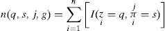
While generalizing NPFLDF, we have n number of non-class feature variables and a single class variable within the dataset D. We can easily reduce this simple point estimation into a generalized maximum a posterior inference notation as below:

A discriminant function is decomposable if its expression is convertible to a sum of local scores, where local score refer to a feature (query) variable in pursuit of drawing graph G. The simple calculation between two feature variable is shown in equation 29. An extended version of this equation can be expressed as ∑j=1qi∑k=1r1Nijk Where i is feature iterator, j is parent iterator, k is feature state iterator and c is class iterator. If we include the factor of class variable, a minor change will be developed into ∑j=1qi∑k=1r1Nijck. Plugging this value into equation 32, we can express as

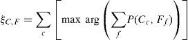
If the feature set is denoted by F={f1, f2, f3,… fn} then ordering weight of any feature will be determined by weight factor shown in equation 34.
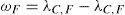
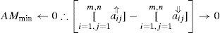
The terms ¿C,F and ¿C,F play the role of existence restrictions. We shall consider both of them as existence restrictions such that (F,C) ∈ ¿C,F: the link F→ C explains the discriminant objective with respect to the class and (F,C) ∈ ¿F,C : the link F← C means the discriminant score with respect to the feature. In our earlier research, we highlighted the correct topological ordering between two features. This was shown by an earlier version of the proposed discriminant function in which we highlight that majority of the discriminant functions can't precisely capture the casual relationship between two variables in pursuit of true topology in numerous situations; this ultimately leads to the selection of potential neighbor and parents becoming unreasonable. However Integration to Segregation (I2S) is capable of rightly identify it in majority of the cases as compared to BIC, MDL, BDeu, Entropy and many more [26], [27]. Moreover, Naeem et al. [26], [27] described that a structure in which class node is placed at the top most may lead to higher predictive accuracies. This type of scheme was termed as “selective BN augmented NBC” [26], [27]. It means that the later score value must be eliminated from the first value which will result into a weighted score vector as shown in the equation 35.

A function for simple descending order is applied to the weights achieved from the equation 35 which results into an ordered list of input variables.

Plugging this ordered set into the equation 33 will give result in
the equation three gives us the discriminant function to be used in the BBN structure learning. In the next section we shall discuss about its performance comparison.5Empirical Validation of Proposed Discriminant function
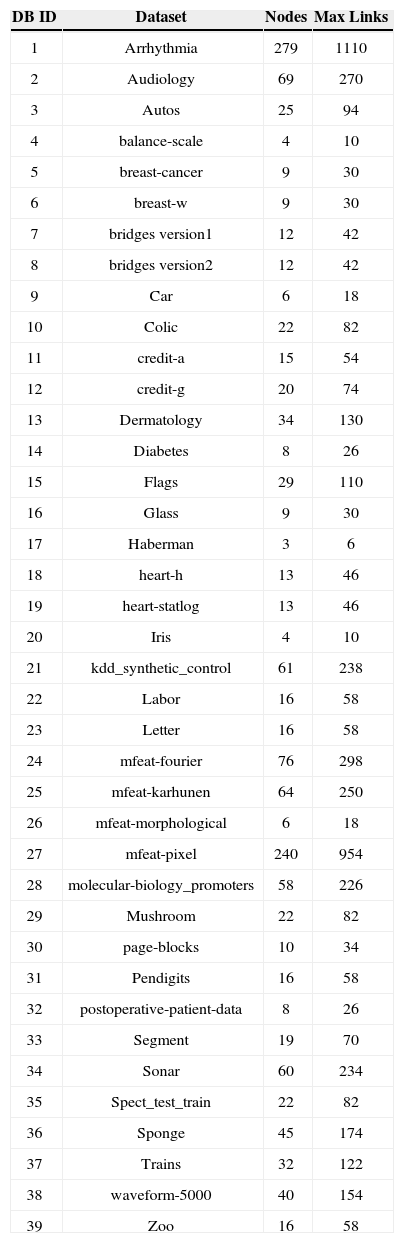
We first obtain thirty nine natural dataset from UCI [20]. These datasets were quite diversified in their specifications. The number of attributes, instances, classes were ranging from small to large value so that any possibility of biasness in the dataset in favor of the proposed metric can be avoided off. The detail is shown in the table 1 We in this experimental study select some of basic meta characteristic and then two enhanced meta characteristics and one of our proposed metrics. The simple meta characteristics include number of attributes, class count and size of cases which are also shown in the table 1. The advanced meta characteristics of dataset include Entropy, Mutual Information and our proposed measure (AMfDS) also technically falls in this category. Before we proceed for analysis, it is mandatory to pre process or transform the data, there are many transformations applicable to a variable before it is used as a dependent variable in a regression model.
Description of dataset used in this study [Parent count constratint (P)=4].
| DB ID | Dataset | Nodes | Max Links |
|---|---|---|---|
| 1 | Arrhythmia | 279 | 1110 |
| 2 | Audiology | 69 | 270 |
| 3 | Autos | 25 | 94 |
| 4 | balance-scale | 4 | 10 |
| 5 | breast-cancer | 9 | 30 |
| 6 | breast-w | 9 | 30 |
| 7 | bridges version1 | 12 | 42 |
| 8 | bridges version2 | 12 | 42 |
| 9 | Car | 6 | 18 |
| 10 | Colic | 22 | 82 |
| 11 | credit-a | 15 | 54 |
| 12 | credit-g | 20 | 74 |
| 13 | Dermatology | 34 | 130 |
| 14 | Diabetes | 8 | 26 |
| 15 | Flags | 29 | 110 |
| 16 | Glass | 9 | 30 |
| 17 | Haberman | 3 | 6 |
| 18 | heart-h | 13 | 46 |
| 19 | heart-statlog | 13 | 46 |
| 20 | Iris | 4 | 10 |
| 21 | kdd_synthetic_control | 61 | 238 |
| 22 | Labor | 16 | 58 |
| 23 | Letter | 16 | 58 |
| 24 | mfeat-fourier | 76 | 298 |
| 25 | mfeat-karhunen | 64 | 250 |
| 26 | mfeat-morphological | 6 | 18 |
| 27 | mfeat-pixel | 240 | 954 |
| 28 | molecular-biology_promoters | 58 | 226 |
| 29 | Mushroom | 22 | 82 |
| 30 | page-blocks | 10 | 34 |
| 31 | Pendigits | 16 | 58 |
| 32 | postoperative-patient-data | 8 | 26 |
| 33 | Segment | 19 | 70 |
| 34 | Sonar | 60 | 234 |
| 35 | Spect_test_train | 22 | 82 |
| 36 | Sponge | 45 | 174 |
| 37 | Trains | 32 | 122 |
| 38 | waveform-5000 | 40 | 154 |
| 39 | Zoo | 16 | 58 |
These transformations can not only restrict towards changing the variance but may incur alteration in the units of variance to be measured. These include deflation, logging, seasonal adjustment, differencing and many more.
However, the nature of data in our study require to adopt the normalization transformation of the accuracy measures and the specific characteristics for which analysis is required. Let xi denotes the accuracy of ith dataset by any classifier then the normalized accuracy can be obtained by the equation as below:

Where

The next step is to obtain a pair wise list with sorting performed on yi such that we denote the sorted list as yi←. With the application of this normalization, a set of normalized characteristics was prepared which was used later on to generate a regression model. A linear regression model is quite useful in order to express a robust relationship between two random variables. The linear equation of regression model indicates the relationship between two variables in the model. Y is regressand or simply a response variable whereas X is regressor or simply an explanatory variable. The output regression line is an approximate acceptable estimation of the degree of relationship between variables. One important parameter in linear regression model is co efficient of determination also known as R-squared. The closer this value to 1, the better the fitting of regression line is represented. R-squared dictates the degree of approximation of the line passing through all of the observation.
Wolpert and Macready [28] stated in their ‘No Free Lunch Theorem’ that no machine learning algorithm is potent enough to be specified outperforming on the set of all natural problems. It clearly points out that every algorithm possesses its own realm of expertise albeit two or more techniques may share their realm in partial. Ali et al., [29] shows that classifiers C4.5, Neural Network and Support Vector Machine were found competitive enough based on the data characteristics measures.
The significance of R-squared is dictated by the fraction of variance explained by a data model but question arises what is the possible relevant variance requiring a suitable explanation. Unfortunately it is not easy to fix a good value of R-squared as in most of the cases, it is far off to get a value of 1.0. In general it is assumed that a value greater than 0.5 indicates the noticeable worthiness of the model. However, still it is a matter of choice as in case of comparison between various models (such as in ours) a more higher value of R-squared counts.
Figure 1 shows the R-Squared values of various linear regression model using specific meta classifiers. Two highest values plotted against AMfDS show the substantial model fitting. These curve fitting were tested with many flavors of regression models ranging from 1st degree to 10th degree order polynomial, 1st order logarithm to 5th order logarithm, polynomial inverse and a lot of special cases data fitting model provided in the commercially available tool DataFit [30]. We noticed that the best curve fitting was found for tenth order degree polynomial regression model.

Decision Stump and Adaboost Decesion Stump both can be explained by the number of classes, joint entropy and proposed metric AMfDS. One the other hand, the data characteristics such as number of attributes and Mutual Information (natural logarithm) can't explain it properly. Moreover, the number of cases (instances) can also explain the accuracy of these classifiers for all of the natural dataset used in this study. We calculated the average joint entropy of each attribute with class attribute; hence the final score is indicative of a score of entropy towards the class variable. The root cause lies in the splitting criterion which is characterized by entropy inspired measure.
Mutual Information (MI) which is an information theoretic measure. MI is basically an intersection of entropy of two features. MI strictly defines the mixed relationship of two variables by which both of them are bound to each other. However we noticed that it did not show up better as compared to other meta characteristics.
Moreover, it is noticeable that AMfDS metric incur significant R-squared value in case of Decision Stump (DS) and its implementation with Ada Boost DS. The R-squared value was 0.875 and 0.836 respectively. It clearly indicates that the classification accuracy of both of these classifiers can be greatly predicted a prior by using AMfDS. It is noticeable that no other meta feature deliver this level of R-squared confidence of determination. The regression model parameters were obtained with 99% confidence interval. The tenth degree regression model defined by AMfDS is shown by the equation six as below:
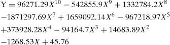
The proposed metric is useless unless it is utilized in a framework. The figure 2 is a typical framework of machine learning in which AMfDS has been plugged. The first two components are preliminary and essential pre requisite for making any data suitable for a machine learner. Once the data is fully prepared, the meta analysis is an essential and novel component where AMfDS will yield an approximated value for the classification accuracy of decision stump. Once the decision is obtained, the end user can find it easily whether this dataset is suitable for this classifier. The regression model gives the accuracy of 87.5% within the confidence interval of 99%. Table 3 is indicating the result we obtained frm our proposed discriminant function NPFLDF. Table 3 indicates that the introduced discriminant function exhibits better in numerous cases. The average accuracy of the proposed function is also better than the other discriminant functions. The last row of the table 3 (‘w’ stands for win and ‘n’ stands for neutral) points out that NPFLDF delivers best result for eleven dataset and for five datasets it shares the best result status with other peer functions. The performance of other functions is quite inferior to that of the proposed function. However if we analyse the results in term of the average accuracy of the functions over all of the datasets then a cynical view on these results indicate that the average accuracy for NPFLDF, AIC, MDL, Bayes and BDeu is almost close to each other but what is the point of difference? The difference is in the model size. The model size in the table 3 ranges from 1 to 100.

A value of 100 means that the model is composed of all of the posible links. For example the dataset ‘arrhythmia’ contains 279 attributes (query variables or nodes in BBN) and one class variable. If we keep the constraint of four as the maximum number of parent nodes then the DAG will have 1110 links. A value of 44.86% (BDeu) means that the model produced by BDue contains 1110×44.86%=498.
If we proceed for further analysis then we noticed that the model size for MDL is small (Average is 36.2) but this size is even more smaller in case of the proposed function where the average model size is 30.03. The worst performance in this dimension of analysis is exhibited by Entropy (Average size is 81.76) wherein this factor is in the range of 50% for the rest of the discriminant functions. The reason behind it is that whenever a new arc is included then the increase in the disciminant effect is only affected if the contributor query variable can increase the class-variable-explanatory effect significantly. However, the searching algorithm K2 also suffers from feature ordering problem. It is a good practice if a feature ranker can order them in such a way that the explanatory features gets more close to the 1st layer of the dag. Here we asume that the top most layer of the DAG is comprised of only class variable; wherein the second layer is comprised of all features. If the process of additions of layers is stopped here then such a BBN is a simple network and it usually gives reduced classification accuracy because of por goodness of data fitting. We in previous sections demonstrated that addition of new arcs (in further layers) influence the goodness of data fitting abruptly. The discriminant functions such as Entropy and AIC usually prone in this category and produce dense network. The problema with such dense network is two folded. Firstly, it requires more computational resources during parameter learning for the sake of inference from BBN. The second problem is model overfitting problem which sharply reduces the classification accuracy. Table 3 shows the same in case of dataset ‘flags’ and ‘kdd_synthetic_control’ where phenomenon of overfitting has explicitly reduced the classification accuracy of test instances.
The figure 3 gives the explanation from different angle in which we obtained the ratio of classification accuarcy and mode density (both in percentage). The calculation was obtained from the equation eight where the value of the constraint (maximum parent node) was set to four. It is evident from the figure 3 that the proposed discriminant function outperforms the other functions (the top curve). The behaviour of entropy was not much promising wherein MDL also give better result after the proposed function.

We have discussed large number of results with various possibilities. However, it is required that we address two simple questions. Why NPFLDF fails in some datasets? What is the justification of results when NPFLDF outperforms? We shall discuss four dataset. These datasets include flags, mfeat-morphological, mfeat-pixel and waveform-5000. All of them vary in their characteristics including attributes, size of the datasets and number of classes. We observed that the datasets with more than two dozen attributes pose computational problems if we set the limit of maximum parent nodes of more than four. The experiment has been performed with setting of maximum node of two, three and four. The noteworthy aspect is that accuracy of NPFLDF was constant in all of the cases. The underlying reason is that the likelihood factor is never getting increased quickly. Usually every segment of the DAG is restricted to two or three nodes while the value of NPFLDF reaches its culmination point. Here the culmination point refers the highest value of NPFLDF for which the goodness of the model is achieved. When we examine the other discriminant functions, this is not the case in most of the situations. We observed that two discriminant functions AIC and Entropy both are drastically accepting nodes under the independence assumption. The performance of entropy in datasets flag (features=30) and mfeatpixel (features=241) is suffering from very large size of conditional probability table. However, the performance of MDL, BDeu and BIC is different. Although these discriminant functions control the unnecessary addition of arcs but usually elimination of wrong orientation is not guaranteed. The behavior of these discriminant functions is implicitly a function of count of parents and unluckily in most of the cases it is erratic. This leaves the problem of “selection of best maximum size of set of parent nodes/features”. However in case of NPFLDF, its embedded characteristics of ordering features ensure to provide the best features for maximizing the discriminant objective. On the other hand, there are situations when NPFLDF did not give better results in comparison to other discriminant functions. The reason can be explained from the figure 3 in which slope of NPFLDF is drastically declining but up to two or three best features. If we reduce the sharpness of this slope then NPFLDF will start tend to go in favor of more features (in this case more than three). However what is the trade between reducing the degree of slope of NPFLDF versus increasing the links to more features. The answer lies in the experimental evaluation. The experimental results in this section point out that if we chose datasets with varying meta characteristics then sharp slope of NPFLDF is more favorable in most of the cases dealing real datasets.
6ConclusionBBN has shown its appealing characterstics in data modeling for causal and noncausal dependencies among a set of data variables. Learning structure out of observational dataset is challenging because of the the model misspecification and nonidentifiability of the underlying structure. In this study, we first tweaked out the affinity relation between two dataset which determines how much one variable can explain the other variable. Keeping in view of it, we fomalized an Affinity Measure which can serve as a meta characteristics for the prediction of classification accuaracy of Decison Stump. the crux of this study was the introduction of a better discriminant function which can learn the BBN structure giving a smart model (reduced complexity in terms of number of arc) while keeping the same or better accuaray of the BBN classifier.