Assessing the Value of Delay to Short-Haul Carriers

Abstract

This paper aims at examining the commercial vehicle operators' value of delay (VOD) due to highway congestion in urban area. The VOD is a fundamental parameter that influences the private sector's response to public freight projects and policies. This paper adopts two methods to estimate the VOD; one being the stated preference (SP) survey and the other being simulation of a carrier's fleet operations. The former applies a Logit model and estimates a driver perceived VOD as $56.48 per vehicle per hour for the regular short-haul delivers. The latter gauges the economic impact of delay on carrier's fleet operations in the Houston highway network. The operations essentially reflect more of a just-in-time system due to the rather stringent time window constraints. The simulation is conducted on a rolling time horizon with a heuristic algorithm for dispatching trucks. The major findings include, but are not limited to as follows. The drivers paid by miles perceive a significantly higher VOD than the others; the drivers are more willing to pay for a faster trip when the toll charges do not come out of their own pockets; VOD increases with uncertainty and demand for capacity. The comparison between the survey and the simulation results also indicates that the interviewed drivers perceive a significantly lower VOD than they may actually experience as a fleet, an indicator of myopic vision.

1

Introduction

The freight delay has a direct and significantly impact on vehicle working hours, fleet efficiency, and the scheduling of warehousing activities, all having a cost implication to the national economy. Unfortunately, with the rapid growth of trucking demand (Federal highway Administration, 2006) and a lagging improvement in the road capacity in the United States, the freight delay due to highway congestion is expected to exacerbate. In the process of developing strategies and policies to mitigate freight delay, the evaluation of the value of freight delay often appears to be a fundamental issue. One example for this is congestion pricing, which is originally designed to divert partial traffic to alternative routes by imposing tolls (Sullivan, 2000, 2002; Supemak et al., 2001; Swenson et al., 2001). An underlying assumption is that the driver's diversion behavior onto alternative routes depends largely on how they value the time savings from avoiding highway congestion.

Another example is prioritizing roadway capacity improvement projects: which bottleneck has the most cost to carriers or truckers? Thus, an accurate understanding of the value of freight delay will enable planners and managers to make informed decisions, leading to improved satisfactions from stakeholders.

2

Literature review

Value of time (VOT) or value of time savings can be viewed as the opportunity cost of travel time. It is typically measured by the maximum amount of money travelers are willing to pay for saving a certain amount of travel time. Since the 1950s, due to traffic congestion in urban areas, there have been numerous studies on the VOT for commuters. These studies primarily aim at the effect of reducing peak hour traffic congestion. Some recent studies can be seen from the work ofHensher and Goodwin (2003), Small et al. (2005), and Fosgerau and Engelson (2011).

However, the commercial value of freight time savings is quite different from that of the commuters. The benefit of freight travel time reduction includes not only the directly reduction in vehicle operating cost but also the improvement in inventory cost due to lesser freight holding and transit time variation, especially for the just–in–time (JIT) system where a strong consideration on delivery time window is imposed. Therefore, the commercial value of time is inherently related to relevant logistics strategies. The Hague Consulting Group (1992, 1995, 1996) conducts a series of early studies to measure the value of freight reliability and delay. In Wigan et al. (2000), commercial VOT is estimated as 1.40 Australian dollars per hour per pallet for metropolitan multidrop freight services in Australia. Further study (Wigan et al., 2003) shows that the value of freight delay for urban less than full truck load (LTL) services is significantly higher than that of other segments. Among these studies, stated preference (SP) and revealed preference are prevailing methods (Fowkes and Shinghal, 2002). Kawamura (2000) applies a switch point method in which truck drivers are asked a choice between an existing freeway versus a toll facility with different combinations of travel time and toll, which is actually a willingness–to–pay study. Together with the survey data at the University of California, Irvine, from the year 1998 to 1999, Kawamura successfully identifies switch points of choosing between different road facilities. The average VOT for truck drivers is found to be $26.8 per hour with a standard deviation of $43.7 per hour. Through grouping, it is also found that hourly waged drivers have higher value than the monthly paid. Overall, there are very limited survey–based studies have been conducted in the United States due to the difficulty in collecting data from truck drivers. Figliozzi (2007) explores the efficiency of urban commercial vehicle operations by disaggregating routing characteristics. Suggestions on data collections and policy implications are made. In his later work (Figliozzi, 2010), numerical experiments are conducted to examine the impact of congestion in terms of tour changes due to time windows. Although the problem is simplified to the extent where the vehicles are assumed to experience the same level of congestion at all points, no quantified results on the value of time/delay are derived.

If direct fuel cost and labor cost (e.g., driver wages) are the only considerations, an existing report suggests an average of $20.23 per hour (American Association of State Highway and Transportation Officials, 2003). Other sources, however, indicate different practical values. For example, Highway Economic Requirements System (HERS) indicates a varying truck VOT from $28.50 to $41.25 per vehicle per hour (Federal highway Administration, 2006). It is also worth to mention that the VOT is estimated significantly higher when considering total logistics costs in the work of ICF Consulting (2002), where the savings in transit time ranges from $144 to $192 and non-scheduled delay is estimated to cost $341 per hour.

This paper aims at developing better methodology to assess the VOT to commercial vehicles due to highway congestion, which we define as value of delay (VOD). This goal is achieved by stated preference technique and simulation to carrier's fleet operation. The stated preference technique includes survey design and data processing, which is based on conditional logit model with the conventional utility function. The original intention of the survey is to examine both time–sensitive delivers (such as JIT) and regular delivers. However, the truck drivers are not likely to be interviewed when they are carrying time-sensitive load (for example, they may refuse to take survey when they are approached at truck stops because they are short of time). The result is that the majority of the data collected comes from the drivers who are running regular delivers. To compensate this effect, the survey is modified to ask the drivers for their perceived time values by introducing two scenarios. The first scenario assumes regular delivers while the second scenario assumes time-sensitive delivers. To compare with the results obtained from survey, a carrier simulation is conducted. It envisions a fleet of vehicles operating within an urban area providing truckload services to customers. Demands with time windows are continuously generated for pickups and delivers. The parameters being considered are demand location, size and pattern, congestion segment and time window. According to Federal Highway Administration (FHWA)'s Freight Benefit-Cost Study (2004), carrier's VOD is derived from marginal vehicle operating cost subjected to fleet routing re-configurations between congested and non-congested situations.

3

Methodologies

3.1

Stated Preference

Revealed Preference assumes that the value of the time can be revealed by actual consumers' choices. Toll stations are a major data source for Revealed Preference studies. However, this method has a major disadvantage due to the data censorship. It simply means that the data is truncated and therefore hard to reflect the whole picture. This problem also exists in demand forecasting. A better strategy is called Stated Preference, which provides combinations of variables to hypothetically construct new options relative to the existing circumstance. These alternatives are carried through carefully designed survey, which is intended to collect and identify trucker's preference. Each alternative is associated with a travel time and a travel cost. The respondents are asked to make choices based on their experiences and perceived values, including lost wages, inconvenience and etc.

Assuming the value of delay for commercial vehicles is related to time sensitivity in terms of pickup and delivery window, two scenarios are constructed in our survey to reflect different driver behaviors. The first scenario assumes urgent deliveries, where the drivers are assumed to be running 30 minutes late due to congested roadways, while the second scenario assumes regular deliveries that are on time no matter what happens. Both scenarios are followed by the options to gain 15, 30, or 45 minutes of time saved, respectively, through paying different tolls. The toll rates are calculated based on a set of discrete values ($30/hr, $40/hr … $120/hr). For example, in an urgent scenario, the survey would ask the respondent to answer three questions, each question has three options associated different time savings and costs (by using a non-congested toll road). Write-in option is provided if the respondent wants to indicate a different rate (typically zero) than the provided options.

Face-to-face interviews were conducted with truck drivers at highway truck stops around Houston, San Marcos, Dallas, and Fort Worth in Texas as well as Belvidere Oasis, Cottage Grove, Janesville, Mauston, and Racine in Wisconsin. These locations were chosen because they are major cities adjacent to where the Texas A&M University was located. At the beginning the truck drivers were approached when they were filling their fuel tanks outside. However, the survey cannot be explain clearly because of the noisy surroundings. A better place for survey was within the gas store where the truck drivers were paying for their fuels or buying food. The questions were well explained to the respondents and the answers were recorded accordingly. During the interview, the use of ‘toll’ was carefully avoided because many respondents disliked it. A total of 133 drivers with hundreds of records were collected. Among all the respondents, 49% are exclusive short-haul drivers while the rest of them runs both short-haul and long-haul businesses. 71% respondents work for freight companies, leaving only 29% as owner operators. This smaller ratio of owner-operators is due to the difficulty in establishing contacts with them in truck stops, which results in a biased sample that cannot be overcome in this study. Typical cargos include truckload (TL) of wood products, textile products, metals, chemicals, office equipments and machineries.

It is observed that in the second scenario, where the respondents are assumed to running without delay, they rarely choose to pay anything for additional time saving. It indicates the fact that the value of delay is significantly diminished if the travel time is not sensitive anymore. The following analysis, therefore, is built on the first scenario. Note that this study cannot identify the drivers having zero experience on the urgent trip. Therefore, the survey is biased because these drivers may not be able to perceive the time value for the urgent trip correctly.

3.1.1

Conditional logit model

The conditional logit model (MLM) is applied to the survey analysis. Generally speaking, it employs a utility function to exam the relationships between the response variables and the associated regressors.

Consider an individual n choosing among alternatives i in a choice set. Suppose the response Y has a set of values y_i corresponding to each alternative i, where y₁₂<…_|/|; A continuous utility U is assumed to be determined by the response variables in the linear form.

¿ is a m-dimension vector of regression coefficients and ¿ a random error with a logarithmic distribution function F. The relationship between Y and U is then

where ¿_i represents a set of threshold points, and x is individual characteristic. The conditional logit model assumes that variables have a constant impact across alternatives, while the individual characteristics are not constant variables over the alternatives. Let U_ni be the utility decided by both alternative i and individual n. Then the probability that the individual n chooses alternative i is

3.1.2

Maximum likelihood estimation

To obtain the coefficient values, we use the maximum likelihood method. The likelihood function has the form of

The MLE maximizes the logarithmic likelihood:

which is a non-linear objective function. Typical gradient search method such as Newton's method is capable of solving it. The convergence criterion is to terminate when likelihood stops increasing.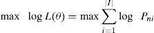

An imbedded PHREG procedure in SAS software is applied for the analysis.

3.1.3

Model fit and utility function

Two different utility functions are tested in this study. The first one is a generic utility function, where the trade-off between cost and travel time is linear:

Where

i = alternatives;

n = individual index;

C_ni = cost specified by individual n in alternative i;

T_i = travel time saving, measured by 0 min, 15 min, 30 min and 45 min;

a, b are coefficients of regressors.

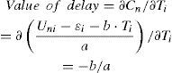
¿_i is unobserved stochastic portion of utility. Note that in the urgent scenario, each respondent should answer three questions, each question is treated as an individual in n. In each question, there are four alternatives (very late, little late, on time, early) associated with different time savings and costs. Only one alternative can be selected for each question. Since mixed logit model is not applied, the following analysis cannot address ‘panel effect’ where the three answers from a respondent are actually correlated. For any i, ¿_i are independent and identical logarithmic distributions. The trucker's value of time is defined as the cost or payment attached to a unit of time saving, which can be derived from the resulting coefficients of regressors. The coefficient a is measured in utility/dollars, and coefficient b is measured by utility/minutes:

The second utility function traces back to the work of Mot et al. in 1989. In order to model the behavior of choosing among the use of cash and checks, they show a non-linear utility function with the payment in logarithm while the other regressors are linear. The use of the logarithm is an empirical choice, and substantially improves the model fit as measured by the log likelihood. Enlightened by their work, the second utility function is proposed:

Due to the logsize of Cni, the equation of value of delay changes to:

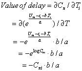
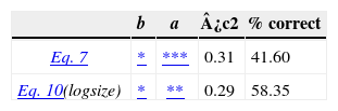
Both utilities are tested using actual survey data. Table 1 shows the comparison between Equation 7 and 9. Statistical fitness details are listed (explanations can be found in Pires et. al, 2012). Although little difference is found in model fit, using Equation 9 would lead to a VOT that is not linear and depends on travel cost (see Equation 10), which is not desired at the planning level because values of time or values of delay must be generic to quantify economic benefits of different transport improvement projects (for example, to calculate the overall benefit by multiplying total hours saved and the dollar value per hour).

Table 1.

Model fit

	b	a	¿c2	% correct
Eq. 7	*	***	0.31	41.60
Eq. 10(logsize)	*	**	0.29	58.35

Number of observations = 399

Adjusted ¿c2=1−LL(¿¿;)−KLL(C)−Kc where

LL(¿¿;) = log-likelihood for the estimated model

K = number of parameters in the estimated model

LL(C) = log-likelihood for the constant only model

K_c = number of parameters in the constant only model

***, **, *

→ significant at 1%, 5%, 10% level

For this reason, Equation 7 was chosen to conduct further analysis over Equation 9. This does not mean that development of Equation 9 is useless. In fact, it can be applied to nonlinearity studies of VOT, but that will not be discussed it here because of the complexity.

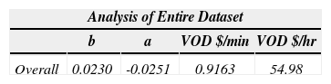
3.1.4

Regression results

Table 2 shows the regression results for the entire dataset using utility function Equation 7. The resulting VOD is first measured by minute and then translated into an hourly value by multiplying 60. Here we do not intend to discuss the issue of linearity of the VOD as previously mentioned.

Table 2.

Analysis using conditional logit model.

Analysis of Entire Dataset
	b	a	VOD $/min	VOD $/hr
Overall	0.0230	-0.0251	0.9163	54.98

Grouping by Survey Area
wisconsin	0.0399	0.0412	0.9684	58.11
Texas	0.0242	-0.0291	0.8316	49.90

Grouping by How Drivers Are Paid
Paid by mile	0.0229	-0.0229	1.0013	60.07
Others	0.0778	-0.1201	0.6478	38.86

Grouping by Who Pays the Toll
Driver pays toll	0.0133	-0.0204	0.6520	39.12
Others	0.0332	-0.0315	1.0540	63.24

Grouping by Type of Carrier
Owner- operator	0.0377	-0.0464	0.8125	48.75
For-hire	0.0079	-0.0184	0.4293	25.76
Private Carrier	0.0312	-0.0321	1.2683	76.10

The overall VOD is estimated to be $54.98 per vehicle per hour. The respondents either operate short-haul exclusively or partially. Thus, the survey result in this study favors the perceived VOD for short-haul operators. To disaggregate different characteristics of the respondents, data are also grouped on survey area, salary method, responsibility of tolls and type of carrier. It is found that the drivers in Wisconsin area perceived a higher VOD ($58.11/hr) than those in Texas ($49.90/hr), possibly due to the different economic structures and population/industry distributions such as fuel price, salary, etc. We also observe that the drivers paid by mile perceived a significantly higher VOD ($60.07/hr) than the drivers paid by other methods, such as hourly salary or per load revenue ($38.86/hr). This is very intuitive because congestion or prolonged travel time reduces total miles traveled. Particularly, the drivers are more willing to pay to avoid delay if the cost does not come out of their own pockets. If the drivers pay the toll by themselves, the VOD is $39.12 per hour; otherwise, it is $63.24 per hour. When comparing private carrier with normal carrier, it is very interesting to notice that the truckers from private carriers perceive a much higher time value. Actually, according to the conversations with our survey respondents, it is indicated that private carrier usually has a tighter schedule because it transports products or materials for its own company and is usually influenced to consider indirect logistic cost, such as fleet optimization and on-time deliver. This finding leads to the next step, which is a fleet simulation to freight carriers.

3.2

Simulation

The stated preference survey is designed to elicit the value of delay perceived by truck drivers. However, it does not necessarily represent the actual VOD to carrier operations. The real VOD should not only include potential lost in fuel and wages but the values of inconvenience, safety, and other psychological factors due to prior expectation and inertia habit. Most importantly, it should consider the potential effect to the other commercial vehicles that are in cooperation. In particular, drivers would tend to decide the value based on their own benefit instead of the effect to the carrier's fleet re-configuration.

In order to gain insights on the re-configuration effect in a coordinated fleet operation, a short-haul truckload simulation is established with the constraints on the time window. Industrial parameters are partially collected through the interviews with local logistic companies and distributors. Additional information is obtained from the survey and online website, such as the possible location for customers or depots, driver wage (fifteen dollar per hour) and etc.

In this simulation, a fleet of vehicles operates within an urban area providing truckload services to customers. Each customer demand has an origin, a destination, and associated time windows for pickup and deliver. Since the travel network is subject to congestion, fleet assignment to drivers is made continuously as demand unfolds with the time of day. The objective is to satisfy the demand with time window and minimize the total operating cost. A Savings Method derived from Solomon (1987) was programmed to make dispatching decisions, which will be explained in details later.

3.2.1

GIS setting

This research uses the ArcGIS database from the National Transportation Atlas Database at the Bureau of Transportation Statistics. 20 locations are selected as potential shipper locations for pickup and delivery according to the business locations in Houston, which reflects a many-to-many operation. Similar setup can be easily modified to address one-to-many case. Truckload demands are generated at each location randomly.

Scenarios based on single depot and double depots are tested respectively. Figure. 1 below illustrates this network.

Figure 1.

Network setting.

The shortest paths between each pair of locations are calculated via ArcGIS. Therefore, the cost matrix and travel time matrix between any two locations are tabulated as input to the simulation. Since the network is mainly constructed by highways, the designed speed is assumed to be 65miles per hour uniformly except on the congestion roads. Several congestion scenarios are tested sequentially in the simulation to compare with congestion free scenario in order to examine the effect of congestion, or say VOD. The data of congestion free situation is obtained by using designed travel speed and distance matrix from ArcGIS. Sparse congestion results in a delay time to the selected segment while pervasive congestion results in a delay to every segment. To decide the potential congestion locations, the traffic information is obtained by using the GoogleMap^TM traffic function. Once congestion is introduced to the scenarios, the shortest paths between locations and depots are re-calculated. Therefore, new assignments of vehicles are made accordingly. Noteworthy is that various congestion situations are created and tested, each corresponding to different cost and time matrices.

3.2.2

Heuristic Algorithm

Although the savings heuristic traces back to Clarke and Wright (1964), the algorithm used in this study is an extension of the savings heuristics proposed in Solomon (1987) for the Vehicle Routing and Scheduling Problems with Time Window Constraints (VRPTW). This is a very popular heuristic method, whose varieties can be found in a wide range of recent literature such as Cedillo-Campos and Sanchez (2013) and Guillén - Burguete et al. (2012).

The algorithm begins with n distinct routes in which each demand is served by a dedicated dummy vehicle from the depot. In the case of two or more depots, a demand is served by a vehicle from the nearer depot. In each step, the tour building heuristic joins two tours with the most saving until no positive saving is possible through joining tours.

Each iteration conducts feasibility check (mainly for time window) of mergers for every pair of existing feasible routes. However, only the two routes with the most saving are chosen to merge. The algorithm terminates when the best saving in current stage is not greater than zero. The general procedure of this heuristics is summarized below.

• Step 0.

  Initialize parameters.

• Step 1.

  Construct initial feasible tours, one for each customer with a designated dummy vehicle.

• Step 2.

  Check feasibility (time window, etc.) of joining each pair of existing tours and record the savings from feasible mergers.

• Step 3.

  If the best saving is positive, join the two according tours, and go back to Step 2. If no feasible merger is available or no positive savings are found from the merger, terminate.

3.2.3

Simulation Framework

The simulation replicates a commercial fleet operating short-haul truckload services in an urban setting. Assignment is periodically done for every two hours. All new demands requested during the previous period are considered and scheduled at the beginning of the next period. If a vehicle is already on the way to pick up or deliver a load, it has to finish that particular demand before committing to another load (dedicated vehicle). Each demand has an origin for pickup and a destination for delivery. Vehicles are allowed to wait at the pickup and deliver location if they arrive early. An example is illustrated in Figure. 2.

Figure 2.

An example daily simulation.

The simulation replicates a commercial fleet operating short-haul truckload services in an urban setting. Assignment is periodically done for every two hours. All new demands requested during the previous period are considered and scheduled at the beginning of the next period. If a vehicle is already on the way to pick up or deliver a load, it has to finish that particular demand before committing to another load (dedicated vehicle). Each demand has an origin for pickup and a destination for delivery. Vehicles are allowed to wait at the pickup and deliver location if they arrive early. An example is illustrated in Figure. 2.

Loading/unloading time is considered to be 30 minutes each. Congestion delay and waiting time is translated to the operating cost based on the driver's salary. Regretful for lacking sensitivity cost, the cost associated with mileage is arbitrarily selected at $2.00 per mile when the vehicle is not in congestion, in order to compromise the results between (American Trucking Association, 2006) and the work done by Fender and Pierce (2012). The output of the simulation is total operating costs required to satisfy the demands in a given congestion level. The difference in cost between scenarios of congestion and congestion free is the congestion cost.

3.2.4

Simulation Results

The congestion cost to the entire fleet operation is based on increased operating hours and distances due to according fleet re-routings to accommodate the expected congestion on highway segments. Assume in a congestion free case where n vehicles need to drive through a particular road segment m times during a day's operation, if congestion occurs at that segment, some of these vehicles have to change their routes while the rest choose to sit in the congestion. The time saved by taking a detour could be put into productive use, but it does not necessarily mean that every vehicle at that segment will take the detour. In fact, the dispatching algorithm controls these decisions because sometimes a detour cost more than waiting in the congestion. The VOD is therefore measured by:

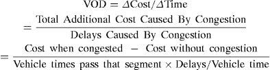
Parameters such as the number of depots, congestion location and pattern (congestion at one segment or at every segment), demand size (number of truckload demands in a day), time window, and demand distribution (the time when demand occurs) are varied during the simulation.

First we test the case with single segment congestion. In this case, two possible congestion locations are considered. One is a 1.22 mile segment on the Gulf Freeway along I45. Another one is located at North Loop along I610 with a length of 1.45 miles. We vary the delay from one minute to thirty. The results show that with one minute delay, the drivers are better off by sticking on the original routes to experience the minor congestion. In the case of congestion longer than three minutes, some trucks begin to move more efficiently by taking an alternative route. This is because our simulation uses the Houston network, where the alternative route takes no more than a few minutes more than the original congestion free route. This network characteristic obviously affects the calculation of VOD. The marginal total additional operating cost is diminishing with the increasing delay due to highway congestion.

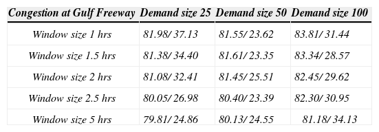
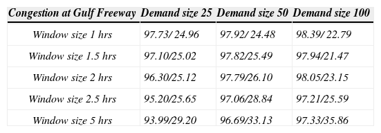
The instances with two minutes delay on chosen highway segments are summarized in Tables 3–5. In Tables 4 and 5, each instance has 20% demands that are already known at the beginning of the day, leaving 80% demands to gradually emerge as the day unfolds and require constantly scheduling update. The instances in Table 5 have 80% demands known before the daily operation begins, which leaves a small portion (20%) to be called in. Table 3 is for one depot and is compared with Table 5, where the demand patterns are different while the traffic condition remains same. Table 4 is for two depots, which shows a VOD from $79.81 to $83.81 per hour.

Table 3.

Central depot (20% known demand)

Congestion at Gulf Freeway	Demand size 25	Demand size 50	Demand size 100
Window size 1 hrs	99.16/22.78	100.03/21.35	100.24/14.15
Window size 1.5 hrs	98.82/25.12	99.83/22.84	100.16/15.63
Window size 2 hrs	98.56/27.16	99.81/27.74	99.38/16.91
Window size 2.5 hrs	98.67/25.09	99.82/28.29	99.62/19.20
Window size 5 hrs	98.25/34.51	98.41/39.50	99.45/31.17

Congestion at North Loop	Demand size 25	Demand size 50	Demand size 100
Window size 1 hrs	102.61/48.92;	117.26/44.57	120.89/22.63
Window size 1.5 hrs	101.36/51.92	117.30/27.20	119.79/22.15
Window size 2 hrs	101.40/52.19	117.06/28.02	118.82/23.77
Window size 2.5 hrs	101.97/52.18	117.25/34.55	120.48/27.37
Window size 5 hrs	99.71/58.84	116.55/32.08	118.24/38.68

Note*Each number is the average of 1000 cases.

Table 4.

Two depots (20% known demand).

Congestion at Gulf Freeway	Demand size 25	Demand size 50	Demand size 100
Window size 1 hrs	81.98/ 37.13	81.55/ 23.62	83.81/ 31.44
Window size 1.5 hrs	81.38/ 34.40	81.61/ 23.35	83.34/ 28.57
Window size 2 hrs	81.08/ 32.41	81.45/ 25.51	82.45/ 29.62
Window size 2.5 hrs	80.05/ 26.98	80.40/ 23.39	82.30/ 30.95
Window size 5 hrs	79.81/ 24.86	80.13/ 24.55	81.18/ 34.13

Table 5.

Central depot (80% known demand).

Congestion at Gulf Freeway	Demand size 25	Demand size 50	Demand size 100
Window size 1 hrs	97.73/ 24.96	97.92/ 24.48	98.39/ 22.79
Window size 1.5 hrs	97.10/25.02	97.82/25.49	97.94/21.47
Window size 2 hrs	96.30/25.12	97.79/26.10	98.05/23.15
Window size 2.5 hrs	95.20/25.65	97.06/28.84	97.21/25.59
Window size 5 hrs	93.99/29.20	96.69/33.13	97.33/35.86

Congestion at North Loop	Demand size 25	Demand size 50	Demand size 100
Window size 1 hrs	98.40/43.60	103.15/30.51	104.68/21.95
Window size 1.5 hrs	98.93/44.14	103.17/32.35	105.28/ 24.12
Window size 2 hrs	98.16/46.58	105.60/33.26	104.39/23.73
Window size 2.5 hrs	96.13/48.17	102.48/35.66	102.48/ 36.98
Window size 5 hrs	94.46/55.47	103.81/44.04	104.14/30.91

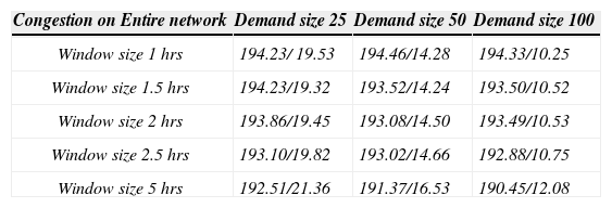
Other than the test of single segment congestion case, we also test a case in which a ubiquitous congestion delay of 0.5 min/mile is applied to the entire network. It is equivalent to reducing the travel speed and is compare with congestion free scenario to calculate additional cost. Table 6 shows the result for this case. The measurement in these tables is dollar/hour. The first number of each cell is the average VOD over 1000 random instances. The second number is the standard deviation over these instances. Each instance is a full day operation with randomly generated demands. The window size indicates the allowable time interval for both pickup and delivery. The demand size represents the number of truckload demands generated during the simulation.

Table 6.

Ubiquitous congestion (80% known demand).

Congestion on Entire network	Demand size 25	Demand size 50	Demand size 100
Window size 1 hrs	194.23/ 19.53	194.46/14.28	194.33/10.25
Window size 1.5 hrs	194.23/19.32	193.52/14.24	193.50/10.52
Window size 2 hrs	193.86/19.45	193.08/14.50	193.49/10.53
Window size 2.5 hrs	193.10/19.82	193.02/14.66	192.88/10.75
Window size 5 hrs	192.51/21.36	191.37/16.53	190.45/12.08

The observations from above tables are described below.

• •

  VOD increases with the demand size. Clearly, congestion is a waste to productivity in general.

• •

  VOD in the case of two depots is at least 25% smaller than in the one depot case. This illustrates that multiple depots are capable of alleviating the congestion impact on freight operations.

• •

  Comparing Table 3 with Table 5 shows a reduced impact from congestion when more demands are known at the start of a day.

• •

  Under the case of ubiquitous congestion (Table 6), the overall vehicle productivity is lowered. The VOD in this case is significantly higher than the other non-extreme cases.

4

Conclusion

In this paper, we make an effort to study the VOD to freight carriers, especially short-haul operators from several perspectives. Our contributions are multifold. First, our study contributes to the very limited literatures that have conducted real world trucker surveys in evaluating freight time value. Second, we appear to be the first to gauge the trade-off between freight time and cost on carriers' operations through simulation, while most of the previous studies solely focus on truckers' perceived value of time. Third, this paper for the first time compares the trucker's perceived value of delay to the simulated congestion cost of carrier's fleet operation. The comparison shows that the truck drivers have a hard time estimating the VOD in the context of supply chain (the simulated values are almost doubled that of the SP). We hope this paper brings attention to the research community of the myriad issues of studying this important topic.

The major findings from the SP survey conducted to short-haul carriers in major cities of Texas and Wisconsin are summarized below.

• •

  VOD is estimated at $54.98 per vehicle per hour.

• •

  The drivers paid by miles perceive a higher VOD than others.

• •

  Private carriers perceive higher VOD than normal carriers.

• •

  The drivers who pay tolls out of their own pockets are less willing to use toll road.

In parallel with the SP survey, an operational simulation is used to assess the cost of congestion to urban short-haul carriers as a fleet. A savings heuristic algorithm is programmed for fleet assignment. The VOD for freight operation is then obtained by comparing the operating costs with and without congestion. Judging by the numbers, the congestion impact for the entire fleet is hardly perceived by individual truckers. The resulting VOD ranges from $93.99 to $120.89 per hour for the case of one central depot. A range from $79.81to $83.81 per hour is estimated for the case of two depots. We find:

• •

  The VOD increases with the growth in number of demands, especially in the case of one central depot.

• •

  The VOD of two depots is smaller than that of one depot, irrespective of congestion location.

• •

  Demand uncertainty and global congestion increases VOD.

It is worth noting that the simulation is conducted with relatively tight time windows when compared with the delivers that are not time-sensitive. This factor plus the fact of being part of private fleet operation within an urban network may inflate the freight time value estimation as an overall average. Through this study, it is realized that to estimate the effect of highway congestion on fleet operation is not an easy task. There are many issues that need to be carefully thought through such as whether and how revenues shall be considered from serving customers, how to set the fleet size to be realistic, how to choose a highway network on which the operation is conducted, and how to consider stochastic travel times. Additionally, the SP method tends to emphasize the trucker's value of time even when the drivers are reminded of the possible fleet effect in survey questions, while the simulation tackles the operating costs from fleet reconfiguration but ignores the driver's will and their myopic views. Nonetheless, we reasonably believe that this study has revealed the general picture on the value of highway freight delay.

Acknowledgment

The authors greatly acknowledge the support from the University Transportation Center for Mobility at the Texas A&M University and the National Center for Freight and Infrastructure Research and Education (CFIRE) at the University of Wisconsin Madison. The authors acknowledge Joshua Levine, Dan Kleinmaier, and Azmy Rajab at CFIRE and Isaac Almy at TAMU for their assistance in collecting and tabulating the survey data.