


The production of soft drinks involves two main stages: syrup preparation and bottling. To obtain the lots sequence in the bottling stage, three approaches are studied. They are based on the sub-tour elimination constraints used in mathematical models for the Asymmetric Traveling Salesman Problem. Two of the mathematical models are from the literature and use classical constraints. The third model includes multi-commodity flow constraints to eliminate disconnected subsequences. The computational behavior of the three models is studied using instances generated with data from the literature. The numerical results show that there are considerable differences among the three models and indicates that the multi-commodity formulation provides good results but it requires far more computational effort when the instances are solved by a commercial software.
Supply chains management has received a lot of attention by practitioners as well as by the research community. The speedup of the computational technology has allowed the incorporation of several aspects of a supply chain into a single model. Chiu et al. [1] studies Economic Production Quantity problem considering multiple or periodic deliveries of finished items. Vanzela et al. [2] address the integration of the lot sizing and the cutting stock problem in the context of furniture production. Another recent trend has been on mathematical models that capture the relationship between the lot sizing and scheduling problems [3]. The so named lot-scheduling models have been proposed for several industrial contexts. For example, the glass container industry [4] and the animal feed supplements industry [5]. It is also considered in the design of virtual cellular manufacturing systems (e.g. [6]).
Two main approaches have been used to model the scheduling decisions. The first one is a small bucket approach in which each period of the planning horizon is divided into sub-periods. For each sub-period only one item can be produced. This approach is based on the GLSP model [7]. The second approach is a big bucket one that allows the production of several items in a given period. Sub-tour Elimination Constraints (SEC) from the Asymmetric Travelling Salesman Problem (ATSP) are added to the lot sizing formulation to obtain the production sequence.
The small and big bucket approaches have been used to model the lot-scheduling problem in the context the soft drink production ([8], [9], [10], [11]). The objective of this work is present a multi-commodity formulation to model the scheduling decisions considering a big bucket strategy. The computational behavior of the proposed model using data from the literature is compared with two other big bucket models presented in the literature, one that uses the SEC proposed by Miller, Tucker and ZEMLIN [10] denominated here by MTZ, and another that uses the SEC proposed by Dantzig, Fulkerson and Johnson [11] denominated here by DFJ.
The paper is organized as follows. In Section 2 the soft drink process and a mathematical model according to literature review are presented. In Section 3 the alternative formulation to model the sequences of lots and an adapted strategy from the literature are presented. Section 4 describes the computational studies and in Section 5 the final remarks are discussed.
2Brief description of previous work for planning the soft drink production processThe production process of soft drinks in different sizes and flavors is carried out in two stages: liquid flavor preparation (Stage I) and bottling (Stage II). The model considers that there are J soft drinks (items) to be produced from L liquid flavors (syrup) on one production line (machine). To model the decisions associated with Stage I, it is supposed that there are several tanks to store the syrup and that it is ready when needed. Therefore, it is not necessary to consider the scheduling of syrups in the tanks, nor the changeover times since it is possible to prepare a new lot of syrup in a given tank, while the machine is bottling the syrup from another tank. However, the syrup lot size needs to satisfy upper and lower bound constraints in order to not overload the tank and to guarantee syrup homogeneity. In Stage II, the machine is initially adjusted to produce a given item. To produce another one, it is necessary to stop the machine and make all the necessary adjustments (another bottle size and/or syrup flavor). Therefore, in this stage, changeover times from one product to another may affect the machine capacity and thus have to be taken into account. In Section 2.1, we review the single stage, single machine model proposed in [10] to define the lot size and lot schedule taking into account the demand for items and the capacity of the machine and syrup tanks, minimizing the overall production costs. It assumes that there is an unlimited quantity of other supplies (e.g. bottles, labels, water).
2.1The lot-scheduling model from literatureIn the model proposed in [10] the decisions associated with lot sizing are based on the Capacitated Lot Sizing Problem (CLSP) (e.g. [12]).
The scheduling decisions use the ATSP approach with the MTZ [13] constraints to eliminate subsequences.
To present the model, let the following parameters define the problem size:J number of soft drinks (items). number of syrup flavors. number of periods in the planning horizon;

Also consider that the following data are known, superscript I relates to stage I (syrup preparation) and superscript II relates to stage II (bottling).
Data:ajII production time for one unit of the item j. changeover time from item i to j. demand for item j in period t. backorder cost for one unit of the item j. inventory cost for one unit of the item j. initial inventory for item j. initial backorder for item j. total time capacity of the machine in t. changeover cost from item i to j. maximum number of tank setups in t. total capacity of the tank. quantity of l for the production of one lot of j. set of items that need syrup I.
Define the following set of variables:Ijt+ inventory for item j at end of period t. backorders for item j at end of period t. production quantity of item j in t. changeover from item i to j in t. might be used to indicated the production order of j in t. number of tanks prepared with l in t. fraction of tank capacity used to produce l in t. is equal to 1 if the tank is setup for l in t.
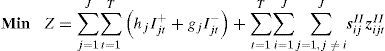
The optimization criterion, Eq. 1, is to minimize the overall costs taking into account inventory, backorder and machine changeover costs.
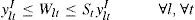
The lot sizing decisions in Stage I, as defined by constraints Eq. 2 – Eq. 5 control the syrup production. Constraints Eq. 2 guarantee that if the tank is ready to produce syrup l, then there will be production of item j and the lot produced uses all the syrup prepared in that period. The variables nlt allow partial use of the tank and controls the minimum amount needed to ensure syrup homogeneity, as specified by constraints Eq. 3. Constraints Eq. 4 ensure that there is syrup production only if the tank is prepared. According to constraints Eq. 5, the total quantity of syrup (in number of full tanks) produced in period t is limited by the maximum number of tank setups.
Stage I - Syrup preparation:


The lot sizing decisions in Stage II are defined by constraints Eq. 6 – Eq. 9. Constraints Eq. 6 represent the balance among production, inventory and backorders of each item in each time period. Constraints Eq. 7 represent the machine capacity in each time period. Constraints Eq. 8 guarantee that there is production of item j only if the machine is prepared. Note that the setup variable is considered implicitly in terms of the changeover variables and that production may not occur although the machine might be prepared. Constraints Eq. 9 control the maximum number of setups in each period.
Stage II (bottling) – lot sizing:

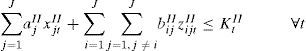


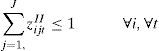
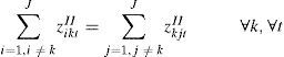
Constraints Eq. 10 – Eq. 14 model the order in which the items will be produced in a given period t. They are based on the ATSP model. Constraints Eq. 10 considers that in each period the machine is initially setup for a ghost item i0. The changeover costs associated with the ghost item are zero and do not interfere in total solution cost. Constraints Eq. 11 guarantee that each item j is produced at maximum once in each period t. Constraints Eq. 12 ensure that if there is a changeover from an item i to any item k then there is a changeover from that item k to an item j.
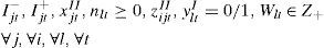
Constraints Eq. 10 and Eq. 12 alone might generate sub-tours, that is disconnected subsequences, and thus do not guarantee a proper sequence of the items. The MTZ type SEC, constraints Eq. 13, avoid this situation. With the inclusion of constraints Eq. 15 the variable ujt gives the order position in which item j is produced in period t. Finally constraints Eq. 15 define the variables' domain.
Stage II (bottling) - scheduling:


The complete description of the model, named here as LSMTZ, is given by expressions Eq. 1 – Eq. 15. More details about this model can be obtained in [10].
3Other strategies to solve the one machine soft drink lot scheduling modelIn the model LSMTZ the constraints associated with the scheduling decisions are formulated based on the MTZ SEC, constraints Eq. 13 and Eq. 14. These constraints are of polynomial order, thus allowing their inclusion a priori. However, the MTZ constraints produce a weak linear relaxation of the associated formulation. Motivated by this fact, several authors have proposed different approaches to strengthen the ATSP mathematical formulation. In the review presented in [14], several mathematical formulations for the ATSP are presented and compared. The focus is on how these formulations compare to one another as regard to the strengthen of the associated linear relaxation.
The multi-commodity-flow formulation proposed by [15] as SEC is equivalent to the classical DFJ ones in terms of the linear relaxation value, and both are better than the MTZ. However, the former, as the MTZ, has polynomial size, while the latter has an exponential size. Next, we explore these two types of constraints to model the ILSP in the soft drink context described in Section 2.
3.1The multi commodity flow based modelThe Multi-Commodity Flow (MCF) formulation is used in [16] to model the scheduling decisions in the presence of non-triangular setups times and costs, and in situations in which the same product can be produced more than once in the same time period.
In this work the MCF formulation is also used to eliminate subsequences in presence of non- triangular setup times, however, as described in Section 2.1 each item can be produced at most once in each time period. The main idea of using the multi-commodity SEC is to obtain a formulation that is stronger than others from the literature, and thus it is expected to have a better computational behavior when solved by general purpose software. A preliminary study of this approach in the soft drink context was presented in [17].
To define the multi-commodity flow formulation, it is necessary to define a new index r ∈ {1, …, J} to represent the commodities and a new set of continuous variables, mrijtII, to represent the flow of the commodity r. The idea behind this formulation is that there are J commodities (items) available at node i0, and a demand of one unit of commodity j at node j. Setting mrijtII=1 implies that if product r is included in the production sequence, then product j follows product i in such sequence. That is, the flow of commodity r flows from node i0 to node r through arc (i, j).
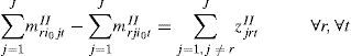
The constraints Eq. 16 – Eq. 19 eliminates disconnected subsequence of items. Since only the items that can be produced should be sequenced, constraints Eq. 16 and Eq. 17 take place when the machine is prepared for item r. These constraints guarantee that if product r is included in the sequence at least one other item should be also included.
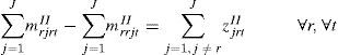
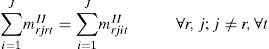
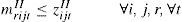
Constraints Eq. 18 are the flow conservation constraints, for all but product r in node r. And constraints Eq. 19 states that item j should follow item i in the sequence that includes item r only if there is a changeover from product i to product j.
The multi-commodity-flow model for the single stage single machine lot-scheduling problem (LSMCF) is defined by the objective function Eq. 1, the Stage I constraints Eq. 2 – Eq. 5, the Stage II constraints Eq. 6 – Eq. 12, the sub tour elimination constraints Eq. 16 – Eq. 19 and the domain constraints Eq. 20.
3.2The DFJ strategy
Besides the MTZ inequalities, the DFJ inequalities [18] were successfully applied to solve a multi machine soft drink process problem. Here, the approach used in [11] is adapted to the single stage, single machine case presented in Section 2. Let C be a set of items that forms a disconnected subsequence. The DFJ type constraints, Eq. 21, eliminate them.

Constraints Eq. 11 ensures that each item is produced at most once per period (i.e., the flow in and flow out of each node (item) is equal to zero or one). For all disconnected subsequences, the following holds:
but ZiktII=1i∈C and k ∈ C. Hence, a solution with a disconnected subsequence does not satisfy constraint Eq. 21.
The LSDFJ model for the single stage single machine lot scheduling problem is defined by the objective function Eq. 1, the Stage I constraints Eq. 2 – Eq. 5, the Stage II constraints Eq. 6 – Eq. 12, the disconnected subsequence elimination constraints Eq. 21 and the domain constraints Eq. 15.
In [4] it is shown that a formulation with this type of constraints is at least as strong as a formulation with the MTZ-type constraints. However, there are an exponential number of constraints Eq. 21. In the computational study presented in Section 4, the DFJ constraints are generated and introduced in the model in a dynamic way (Strategy 2). At first a relaxation of the LSDFJ built by removing constraints Eq. 21 is solved. If the best solution obtained has disconnect subsequences, the constraints Eq. 21 that are violated by this solution are included in the relaxation and it is solved again. Otherwise, the optimal solution has been found and the algorithm halts. The algorithm might also halt if the maximum cpu time allowed is achieved, in this case only a lower bound to the optimal solution is obtained. A feasible solution can be built using heuristics, for example the patching heuristic described in [11].
4Computational StudyThe three models presented in Sections 2.1, 3.1 and 3.2, and the cutting plane algorithm to solve the LSDFJ model have been codified in the AMPL syntax [19]. Two strategies were used to solve the instances of the three models. In Strategy 1 the LSMTZ and LSMCF model's instances are solved by the branch and cut algorithm of Cplex 12.5 [20].
In the Strategy 2 the LSDFJ model's instances are solved by the cutting plane method described in Section 3.2. The mixed integer relaxations in each iteration of the Strategy 2 were also solved by the Cplex 12.5. All the runs were executed on a computer Intel Core i7-2600 CPU, 3,4 GHz, 16 GB RAM.
4.1InstancesTwenty instances (S1-S20) of each one of the three models were used in the computational tests. The data is related to one machine that can produce 27 items of different flavors and bottle sizes. Ten different flavors are necessary to produce this set of items. A planning horizon of five weeks (periods) was considered.
The Table 1 presents the main characteristics of the instances. The instances S1-S10 are from [6]. They have the changeover costs higher than the inventory and backorder costs, even when they are reduced in 25%. To analyze scenarios in which the sequencing decisions are less important than the lot sizing decisions, ten new instances were generated. The changeover costs of instances S1-S10 were reduced, while the inventory and backorder costs were left unchanged.
Main characteristics of the instances.
| Instance | Modifications |
|---|---|
| S1 (S6) | Plant data. |
| S2(S7) | Machine capacity of S1 (S6) reduced by 25%. |
| S3 (S8) | Inventory costs of S1 (S6) doubled. |
| S4(S9) | Machine capacity of S1 (S6) reduced by 25%.Changeover costs of S1 (S6) reduced by 1/3. |
| S5(S10) | Machine capacity of S1 (S6) reduced by 25%.Inventory costs of S1 (S6) doubled.Changeover costs of S1 (S6) reduced by 1/3. |
| S11 (S14) | Changeover costs of S1 (S6) are the changeover times reduced by 1/100,000. |
| S12(S15) | Machine capacity of S1 (S6) reduced by 25%.Changeover costs of S1 (S6) are the changeover times reduced by 1/100,000. |
| S13(S16) | Machine capacity of S1 (S6) reduced by 25%. Inventory costs of S1 (S6) doubled.Changeover costs of S1 (S6) are the changeover times reduced by 1/100,000. |
| S17(S19) | Changeover costs of S1 (S6) are the changeover times reduced by 1/100. |
| S18(S20) | Machine capacity of S1 (S6) reduced by 25%.Changeover costs of S1 (S6) are the changeover times reduced by 1/100. |
Two tests were conducted by changing the Cplex stopping criterion, Test 1 and Test 2. The goal of the Test 1 is to analyze if the use of the multi-commodity SEC constraints (Section 3.1) in a Lot-Scheduling model is better than the MTZ SEC constraints (Section 2.1) to obtain good linear relaxation values and to find good feasible solutions when solved using Strategy 1. So, the runs in Test 1 were interrupted after examining 500 nodes of the Branch and Cut tree. The LSDFJ model was not included in the Test 1 because, as mentioned in Section 3.2, it is has an exponential number of constraints and could be solved only by a cutting plane algorithm.
In the Test 2, the goal is to study the performance of the three models when used as tool to solve the ILSP problem in the soft drink context, and so a maximum of 3 hours of CPU time was allowed in each run.
4.2.1Test 1: maximum 500 nodesThe value of the linear relaxation associated to all the 20 instances of the LSMTZ and LSMCF models were the same. However, the time spent to solve them is longer for the LSMCF instances (0.2 seconds) than for the LSMTZ ones (0.02 second).
After examining 500 nodes of the branch and cut tree, the Cplex returned solutions for the S1-S10 instances of the LSMTZ model with average gap of 82.55% and for 90% of the instances the confidence interval of the gap is [68.65% – 96.46%]. Cplex returned better solutions for all the ten instances of the LSMCF model. The average gap is 14.38% and for 90% of the instances the confidence interval is [7.99% – 20.77%], which represent an important reduction in the gap value. However, in relation of the cpu time, Cplex spent more time with the LSMCF instances (1,530.50 seconds in average) than with the LSMTZ instances (an average of 2.82 seconds).
As for the instances S11-S20, the average gap of the solutions obtained with the LSMTZ model is 99.53% and with the LSMCF model is 0.34%. The computational time of Cplex for the instances of both models is smaller than the computational time of the first set of 10 instances solved, but the time for the instances of LSMTZ model is smaller, 1.32 seconds in average, while the average for the LSMCF instances is 499 seconds. This results shows that the LSMCF model is better than the LSMTZ model in terms of solution quality and worse in terms of computational effort.
4.2.2Test 2: maximum cpu time of three hoursIn the Test 2, cpu time limit of a maximum of 3 hours, the Cplex Branch and Cut algorithm examined an average of 3 million nodes to solve the LSMTZ instances against 7 thousand nodes for the LSMCF instances. As a result, more cuts were generated and applied when solving the LSMTZ instances (an average of 15,043 cuts) than when solving the LSMCF instances (an average of 4,392). This performance of the models was expected because of the Test 1 results in which for the instances of the LSMTZ models, Cplex examined 500 nodes in 2.82 seconds on average while for the LSMCF instances it took much longer. The fact that the LSMTZ instances can be solved easily using the Cplex's branch and cut algorithm might be connected to the fact that the linear relaxations involved are solved 10 times quicker than the ones associated to the LSMCF instances. The same maximum cpu time was imposed for solving the LSDFJ instances using Strategy 2.
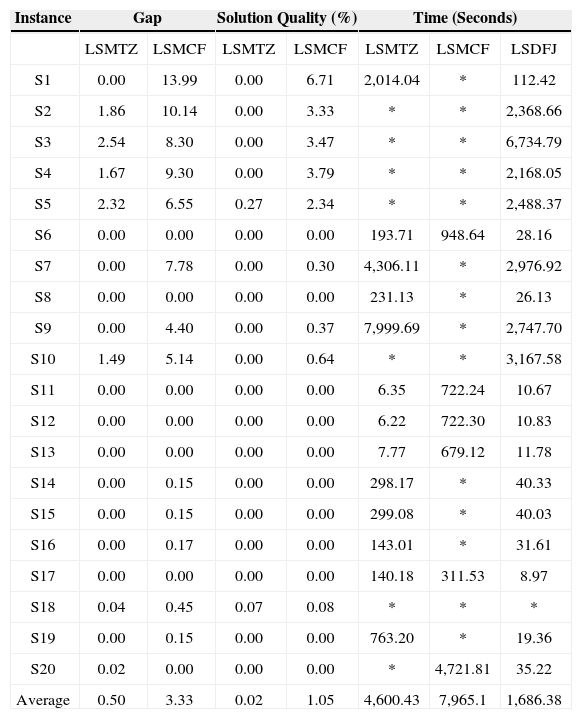
Given that the Strategy 2 provided the optimal solution for 19 of the 20 instances of the LSDFJ model, it is possible to compare the models in terms of best solution quality as well as the gap and cpu times. The solution quality is computed as ((Best solution value) – (optimal solution value))/optimal solution value) * 100), in which the best solution value accounts the best feasible integer solution value found with Strategy 1 for the LSMTZ and for the LSMCF instances. These results were compiled in Table 2. The first column shows the name of each instance, the next two columns show the gap associated to the LSMTZ and LSMCF solutions respectively. The following two columns show the quality of the solutions obtained using Strategy 1 to solve the LSMTZ and the LSMCF instances respectively. The last three columns show the cpu times in seconds to obtain the best solution for all the three model instances. Given that for all but one instance (instance S18), the Strategy 2 provided the optimal solution, the gap is not show for the LSDFJ solutions.
Results for the LSMTZ, LSMCF and LSDFJ models – gap, solution quality and cpu time.
| Instance | Gap | Solution Quality (%) | Time (Seconds) | ||||
|---|---|---|---|---|---|---|---|
| LSMTZ | LSMCF | LSMTZ | LSMCF | LSMTZ | LSMCF | LSDFJ | |
| S1 | 0.00 | 13.99 | 0.00 | 6.71 | 2,014.04 | * | 112.42 |
| S2 | 1.86 | 10.14 | 0.00 | 3.33 | * | * | 2,368.66 |
| S3 | 2.54 | 8.30 | 0.00 | 3.47 | * | * | 6,734.79 |
| S4 | 1.67 | 9.30 | 0.00 | 3.79 | * | * | 2,168.05 |
| S5 | 2.32 | 6.55 | 0.27 | 2.34 | * | * | 2,488.37 |
| S6 | 0.00 | 0.00 | 0.00 | 0.00 | 193.71 | 948.64 | 28.16 |
| S7 | 0.00 | 7.78 | 0.00 | 0.30 | 4,306.11 | * | 2,976.92 |
| S8 | 0.00 | 0.00 | 0.00 | 0.00 | 231.13 | * | 26.13 |
| S9 | 0.00 | 4.40 | 0.00 | 0.37 | 7,999.69 | * | 2,747.70 |
| S10 | 1.49 | 5.14 | 0.00 | 0.64 | * | * | 3,167.58 |
| S11 | 0.00 | 0.00 | 0.00 | 0.00 | 6.35 | 722.24 | 10.67 |
| S12 | 0.00 | 0.00 | 0.00 | 0.00 | 6.22 | 722.30 | 10.83 |
| S13 | 0.00 | 0.00 | 0.00 | 0.00 | 7.77 | 679.12 | 11.78 |
| S14 | 0.00 | 0.15 | 0.00 | 0.00 | 298.17 | * | 40.33 |
| S15 | 0.00 | 0.15 | 0.00 | 0.00 | 299.08 | * | 40.03 |
| S16 | 0.00 | 0.17 | 0.00 | 0.00 | 143.01 | * | 31.61 |
| S17 | 0.00 | 0.00 | 0.00 | 0.00 | 140.18 | 311.53 | 8.97 |
| S18 | 0.04 | 0.45 | 0.07 | 0.08 | * | * | * |
| S19 | 0.00 | 0.15 | 0.00 | 0.00 | 763.20 | * | 19.36 |
| S20 | 0.02 | 0.00 | 0.00 | 0.00 | * | 4,721.81 | 35.22 |
| Average | 0.50 | 3.33 | 0.02 | 1.05 | 4,600.43 | 7,965.1 | 1,686.38 |
The results shown in Table 2 suggest a superiority of the LSDFJ model when compared to the LSMTZ and LSMCF models. The Strategy 2 proved the optimality for 19 instances of the LSDFJ model while the Strategy 1 proved the optimality for 13 instances of the LSMTZ model and 6 instances of the LSMCF model. However, the gap for the instances S18 and S20 of the LSMTZ model are smaller than 0.3% and the solution quality smaller than 0.27% suggesting that these solutions can be considered optimal. The same happens with the instances S14, S15, S16, S18 and S19 of the LSMCF model. The Strategy 2 used to solved the instance S18 of the LSDFJ model halted after three hours without a feasible solution, although the lower bound is 2,371.33.
If we consider the convergence of the solution process used to solve the models instances, the LSMTZ model is better. The Figure 1 shows the solution values for the S3 instance obtained halting the strategies applied to solve it after 10, 20, 30, 40, 50 and 60 minutes of cpu time. The vertical axis shows the solution value, and the horizontal axis shows the cpu time. The LSMTZ solution, for example, provided the optimal solution in 40 minutes but the associated gap is still 4.82%. The LSMCF solution values are far from the optimal value and the gap is still 17.58% after 1 hour. The LSDFJ solution values are close to the optimal value. However, it is important to remember that these solutions are not necessarily feasible or provided a dual bound. For example, when the run was interrupted after 30 minutes, the current relaxation was not solved to optimality. A guaranty of feasibility can obtained at the end of the Strategy 2, when no more subsequences elimination constraints are violated.

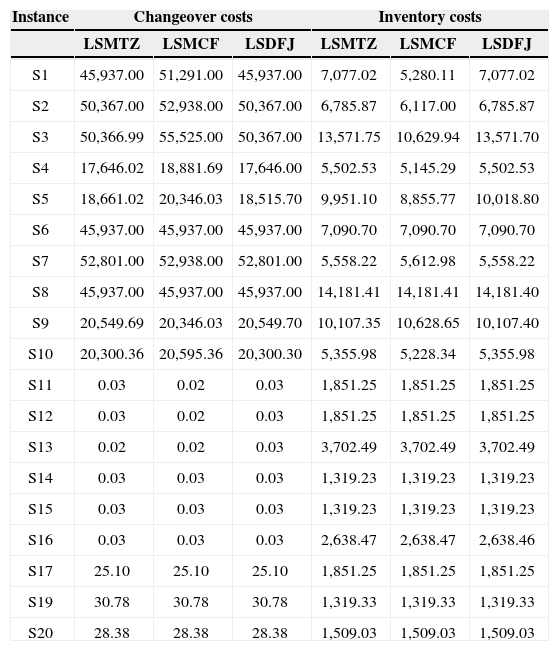
To analyze the effect of the changeover costs on the solution process of the three models, it is shown in Table 3 the solution values in terms of the changeover costs (columns 2 to 4) and the inventory costs (columns 5 to 7). There are backorder costs only for the instances S6-S10. As they are very similar to each other they were not presented in the table. Because of the high changeover costs in the instances S6 to S10 there are backorder costs, even in the optimal solutions.
Solution value in terms of changeover and inventory costs
| Instance | Changeover costs | Inventory costs | ||||
|---|---|---|---|---|---|---|
| LSMTZ | LSMCF | LSDFJ | LSMTZ | LSMCF | LSDFJ | |
| S1 | 45,937.00 | 51,291.00 | 45,937.00 | 7,077.02 | 5,280.11 | 7,077.02 |
| S2 | 50,367.00 | 52,938.00 | 50,367.00 | 6,785.87 | 6,117.00 | 6,785.87 |
| S3 | 50,366.99 | 55,525.00 | 50,367.00 | 13,571.75 | 10,629.94 | 13,571.70 |
| S4 | 17,646.02 | 18,881.69 | 17,646.00 | 5,502.53 | 5,145.29 | 5,502.53 |
| S5 | 18,661.02 | 20,346.03 | 18,515.70 | 9,951.10 | 8,855.77 | 10,018.80 |
| S6 | 45,937.00 | 45,937.00 | 45,937.00 | 7,090.70 | 7,090.70 | 7,090.70 |
| S7 | 52,801.00 | 52,938.00 | 52,801.00 | 5,558.22 | 5,612.98 | 5,558.22 |
| S8 | 45,937.00 | 45,937.00 | 45,937.00 | 14,181.41 | 14,181.41 | 14,181.40 |
| S9 | 20,549.69 | 20,346.03 | 20,549.70 | 10,107.35 | 10,628.65 | 10,107.40 |
| S10 | 20,300.36 | 20,595.36 | 20,300.30 | 5,355.98 | 5,228.34 | 5,355.98 |
| S11 | 0.03 | 0.02 | 0.03 | 1,851.25 | 1,851.25 | 1,851.25 |
| S12 | 0.03 | 0.02 | 0.03 | 1,851.25 | 1,851.25 | 1,851.25 |
| S13 | 0.02 | 0.02 | 0.03 | 3,702.49 | 3,702.49 | 3,702.49 |
| S14 | 0.03 | 0.03 | 0.03 | 1,319.23 | 1,319.23 | 1,319.23 |
| S15 | 0.03 | 0.03 | 0.03 | 1,319.23 | 1,319.23 | 1,319.23 |
| S16 | 0.03 | 0.03 | 0.03 | 2,638.47 | 2,638.47 | 2,638.46 |
| S17 | 25.10 | 25.10 | 25.10 | 1,851.25 | 1,851.25 | 1,851.25 |
| S19 | 30.78 | 30.78 | 30.78 | 1,319.33 | 1,319.33 | 1,319.33 |
| S20 | 28.38 | 28.38 | 28.38 | 1,509.03 | 1,509.03 | 1,509.03 |
The decrease in changeover times and absence of backorder costs in the optimal solution shows that there is capacity available to attend the demand. Moreover, from the results compiled in tables 2 and 3], we note that when changeover costs are smaller (instances S11 to S20) the strategies used to solve the models instances are more efficient and the computational times are significantly reduced.
5ConclusionsIn this paper we studied three formulations for the single stage, single machine lot scheduling problem in the context of soft drink production. The models differ by the set of constraints used to eliminate disconnected subsequences. The models LSMTZ and LSDFJ are from the literature and are based on the classical subtour elimination constraints used in the ATSP models. The LSMCF model is a new contribution and uses the multicommodity flow constraints to model the lots sequence. The LSMCF model has a higher number of constraints to eliminate subtours than the LSMTZ model, but both have a polynomial number of constraints while the LSDFJ model has an exponential number of constraints.
The computational results obtained when the branch and cut tree of the Cplex was limited to 500 nodes shows that the LSMCF model is better than the LSMTZ model in terms of solution quality and worse in terms of cpu time. The difficulty of the LSMCF model is that the time spent to solve the associated linear relaxation is 10 times longer than the time necessary to solve the LSMTZ linear relaxation.
The results obtained allowing 3 hours of cpu time to solve the models instances show that the LSMTZ model provides better solutions than the LSMCF model. This is explained considering that with this time limit it is possible to examine a higher number of nodes in the branch and cut tree of the LSMTZ instances. The results obtained using the LSDFJ model are even better. It was possible to prove optimality to all but one of the 20 instances tested when solving the LSDFJ model instances by the cutting plane method. A disadvantage of this strategy is that there is guarantee of feasibility only at the end of the procedure. Considering these results, the LSMTZ model can be considered the best one. It provided competitive solutions in a reasonable computational time. For scenarios in which the changeover costs are small the strategies used to solve the three models instances are efficient and the computational times are significantly reduced when compared to scenarios with high changeover costs.
This research was partly supported by the Brazilian research agencies CNPq (306194/2012-0) and Fapesp (2010/19006-0, 2013/07375-0, 2010/10133-0).