


Las pérdidas económicas debidas a desastres naturales se han incrementado en las últimas décadas como resultado del desarrollo socioeconómico y probablemente del cambio climático. Las proyecciones indican que esta tendencia al alza continuará, lo cual resalta la necesidad de adoptar estrategias de adaptación. Esto a su vez pone de manifiesto la necesidad de establecer mejores estrategias de adaptación adecuadas para hacer frente a los embates inciertos del cambio climático. El presente estudio muestra cómo puede aplicarse una cascada de modelaciones de riesgo y desastres, y un análisis de costo-beneficio, para obtener un primer indicador de estrategias de adaptación eficientes desde el punto de vista económico. Este enfoque se aplica a un análisis de riesgos de inundación y a la conveniencia de contar con protección contra inundaciones en el estado de Tabasco, México, el cual padece graves inundaciones casi anualmente. Los resultados muestran que el daño anual esperado por inundaciones costeras se incrementará de los actuales USD 530 millones a USD 4120 millones en 2080 como resultado del desarrollo socioeconómico y el cambio climático. En cuanto al daño estimado por inundaciones fluviales, se espera que se incremente de los actuales USD 1790 millones a USD 10 600 millones en 2080 si no se establecen medidas de adaptación. Con base en el análisis de riesgo y costo-beneficio de la construcción de infraestructura contra inundaciones, establecimos en al menos 100 años los estándares óptimos de protección desde el punto de vista económico para ambos tipos de inundación. Nuestras principales conclusiones son robustas con relación a la incertidumbre sobre los efectos del cambio climático en riesgos de inundación, los daños indirectos causados por éstas, la extensión de los terrenos inundables y la tasa de descuento social adoptada. Analizamos la forma en que nuestro enfoque multidisciplinario puede ayudar a los encargados de la toma de decisiones respecto al manejo de riesgos de inundación, y la manera en que investigaciones venideras pueden ampliar nuestro método a análisis locales específicos, que son necesarios para desarrollar planes de adaptación a nivel local.
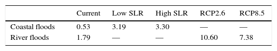
Economic losses as a result of natural hazards have been rising over the past few decades due to socio-economic development and perhaps climate change. This upwards trend is projected to continue, highlighting the need for adequate adaptation strategies. This raises the question of how to determine which adaptation strategies are preferred to cope with uncertain climate change impacts. This study shows how a multi-disciplinary cascade of hazard modelling, risk modelling, and a cost-benefit analysis can be applied to provide a first indicator of economically efficient adaptation strategies. We apply this approach to an analysis of flood risk and the desirability of flood protection in the state of Tabasco in Mexico, which faces severe flooding on an almost yearly basis. The results show that expected annual damage caused by coastal flooding is expected to increase from 0.53 billion USD today up to 4.12 billion USD in 2080 due to socio-economic development and climate change. For river floods, expected annual damages are estimated to increase from 1.79 billion USD up to 10.6 billion USD in 2080 if no adaptation measures are taken. Based on the estimated risk and cost-benefit analysis of installing flood protection infrastructure, we determined the economically optimal protection standards for both river and coastal floods as at least 100 years, if we take into account climate change. Our main conclusions are robust to key uncertainties about climate change impacts on flood risks, indirect damage caused by floods, the width of the protected floodplains, and the adopted social discount rate. We discuss how our multi-disciplinary approach can assist policy-makers in decisions about flood risk management, and how future research can extend our method to more refined local analyses which are needed to guide local adaptation planning.
Economic losses from natural disasters have been increasing during the past few decades in many areas around the world (IPCC, 2012). This upwards trend in losses has been mainly attributed to socio-economic developments, such as economic and population growth in disaster-prone areas, which have increased the exposure of properties that can be damaged by natural hazards over time (Bouwer, 2011). Natural disaster damages are the outcome of a complex interplay of these changes in exposure with changes in vulnerability, caused by socio-economic development and decisions, and changes in hazard, which can be influenced by climate change or human interventions in the hydrological system. These interactions make it complicated to draw clear-cut conclusions on trends in the causes of natural disaster losses. It cannot be ruled out that climate change has contributed to past natural disaster losses (Estrada et al., 2015). Moreover, future natural disaster losses are expected to increase in many regions around the world (Hirabayashi et al., 2013). Future risks are projected to increase due to a combination of continued population and economic growth and climate change, which can cause increases in the frequency and/or intensity of extreme weather events, such as more severe droughts, storms, and floods (IPCC, 2014).
The projected increase in risks from natural disasters can be limited by implementing adaptation measures, such as installing protection infrastructure and adjusting buildings so they can better withstand the disaster. A key question is thus how to identify adaptation measures that are suitable for the local scale and which generate an adequate economic return. An interdisciplinary approach of hazard assessment, risk assessment, and economic cost-benefit analysis (CBA) of adaptation measures can provide insights for identifying economically efficient adaptation strategies to manage natural disaster risk, as will be illustrated in this study. In short, natural hazard modelling involves estimating potential hazard characteristics in terms of physical variables, such as potential flood extents and inundation depths in an area (e.g. Chen et al., 2016). As a next step, risk modelling aims to estimate the societal impacts, usually in terms of property damages, that are associated with specific hazard characteristics; for instance, the potential damage that a flood can cause in a certain geographical area (Grossi and Kunreuther, 2005). The low-probability nature of natural disasters generally means that few historical data exist on disaster impacts, which explains why most natural disaster risk assessments rely on models to estimate how hypothetical hazard characteristics translate into monetary damages. This can be carried out in a modelling framework, often using a Geographical Information Systems (GIS) environment that combines hazard-modelling output with information about exposed land use or property values and assumptions about their vulnerability, i.e. their susceptibility to damage. Common outputs of risk models include the potential direct property damage and/or indirect business interruption damage that a particular hazard can cause (such as a flood with a certain probability), or the expected annual damage (EAD) of a hazard (e.g. Meyer et al., 2013). When such risk indicators are presented at a high spatial resolution they can be used for indicating where risk management measures, for example flood protection infrastructure, should be prioritised (Zerger, 2002). Moreover, risk modelling can deliver key inputs for CBA of disaster risk reduction strategies by estimating the potential benefits of such measures, in terms of the reductions in EAD they deliver, as shown by Michel-Kerjan et al. (2013) in a developing country context, and by Aerts et al. (2014) for global megacities. A CBA can be used for evaluating whether the benefits of a risk management measure outweigh the costs over its lifetime, with the aim to identify economically desirable natural disaster risk reduction measures (Mechler, 2016). Accounting for the potential impacts of climate change on natural disaster risk in the CBA allows for the examination of economically efficient strategies to adapt to changing risks. Such an analysis is evidently complicated by uncertainty, such as the uncertain climate change impacts on natural disaster risks. Here a multi-disciplinary approach will be illustrated, that applies the aforementioned methods for estimating local flood risk levels and the economic efficiency of flood protection strategies to the rivers and coastline of the Mexican state of Tabasco. In particular, in this study we will examine how the economic desirability of flood protection depends on the uncertainty in climate change scenarios and other key assumptions. This analysis delivers insights for flood risk management by showing whether installing flood protection is economically desirable, and by providing a first indication of the optimal flood safety standard, i.e. the flood return period against which the infrastructure should provide protection. Tabasco, located in southern Mexico, is one of the country's wettest areas and is regularly subjected to floods from rivers and storm surge. The state has been flooded yearly between 2007 and 2012, with severe consequences for the region (Section 2). Furthermore, climate change is expected to influence the hydrological cycle, leading to more intense precipitation and sea-level rise (SLR), which could lead to increased flood risk. An illustration of the severe flood conditions that the region faces are the extreme storms and rainfall events that occurred in 2007, which led to the flooding of 60% of the state, including its capital city Villahermosa, and affected approximately 1.5 million people. Our study is motivated by a report written in the aftermath of the storm, on request of the Governor of the state, which recommended conducting a detailed flood risk assessment to aid the adaption and mitigation of flood disasters (EHS-GA, 2008).
The remainder of this paper is structured as follows. Section 2 describes the flooding problem in Tabasco. Section 3 outlines the methodology used for assessing flood risk and the CBA of flood protection strategies. Section 4 presents the results and Section 5 concludes.
2Flooding in the state of Tabasco, MexicoTabasco is located in south-eastern Mexico on the Isthmus of Tehuantepec, which is the strip of land where the distance between the Gulf of Mexico and the Pacific Ocean is smallest (Fig. 1). The state is bounded by the states Campeche in the east, Chiapas in the south, and Veracruz in the west, and by the 184 km-long coastline along the Gulf of Mexico in the north. It also forms a part of the Mexican border with Guatemala in the southeast of the state. Its total surface area is 25 267 km2, representing 1.3% of the total Mexican territory, and it is divided into 17 municipalities. In total, Tabasco has 2 238 603 inhabitants (2010), representing about 5% of the total Mexican population. Of these inhabitants, approximately 55% live in urban areas and 45% in rural areas (CONAGUA, 2010). The capital of the state is Villahermosa, which is home to about 550 000 people.

The amount of precipitation received by Tabasco is the highest of all the states of Mexico, with an average of 2095 mm/year for the period 1971-2000 (Gama et al., 2011). This is predominantly concentrated in the rainy season between June and September, as well as in October and November. Furthermore, the region is regularly subjected to tropical storms and hurricanes from both the Gulf of Mexico and the Pacific Ocean. With the exception of some higher areas in the South, its topography is generally flat and low and is largely covered with lakes, lagoons and wetlands (Encyclopaedia Britannica, 2016), with poor drainage from deltaic and alluvial soils annually exposing the territory to floods (Gama et al., 2011). The hydro-geo-logic conditions are characteristic of a semi-closed aquifer, and rapid saturation of the upper soil layers makes infiltration of the water impossible, causing the majority of the precipitation to be discharged as surface runoff (Perevochtchikova and Lezama de la Torre, 2010). The state is drained by two of Mexico's largest rivers, namely the Grijalva and Usumacinta Rivers, which originate in Chiapas. This system is one of the biggest watersheds in North America and by far the biggest in Mexico, with a catchment area of 83 553 km2. Together, the two rivers account for 30% of all the fresh water flows of the country (Gama et al., 2011). The eastern part of the river system, where the Usumacinta River is located, is not controlled by hydraulic constructions, while in the western part of the system four hydro-electric dams have been built in the Upper Grijalva River. The system discharges in the Lower Grijalva River system and therefore has a significant effect on the coastal plain of Tabasco (Rivera-Trejo et al., 2010).
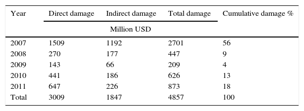
Due to its climatic and hydro-geologic conditions Tabasco is one of the most flood-prone states in Mexico. In the period 2007-2011 the state was flooded on a yearly basis, resulting in a total damage of approximately five billion USD (Table I). The most extensive flooding in the recent past took place in 2007, at the end of October and early November, and affected over 62% of the state and more than 1.2 million people. Although fortunately no loss of human lives was reported, it was the worst flood experienced by the state in 50 years and made a large economic impact with more than three billion USD damage (Perevochtchikova and Lezama de la Torre, 2010).
Direct and indirect damage in Tabasco resulting from hydro-meteorological effects in the period 2007-2011 as reported by the United Nations Economic Commission for Latin America and the Caribbean (CEPAL, 2011).a
| Year | Direct damage | Indirect damage | Total damage | Cumulative damage % |
|---|---|---|---|---|
| Million USD | ||||
| 2007 | 1509 | 1192 | 2701 | 56 |
| 2008 | 270 | 177 | 447 | 9 |
| 2009 | 143 | 66 | 209 | 4 |
| 2010 | 441 | 186 | 626 | 13 |
| 2011 | 647 | 226 | 873 | 18 |
| Total | 3009 | 1847 | 4857 | 100 |
Heavy rains preceded the floods, with maximum daily values of 200-300 mm, which some have argued were the result of the combination of a cold front from the USA and tropical storm Noel (Rivera-Trejo et al., 2010). The maximum accumulated precipitation was more than 1400 mm, and in Ocotepec the precipitation even exceeded 400 mm in one day on October 28. The average precipitation in Tabasco for the month of October is 317.5 mm, which means that the daily rainfall during this event was more than the monthly average for this region. Furthermore, the region had already experienced several other rainfall events during the month of October, causing wet preconditions in the basin and adding to the problems.
Another important factor in the 2007 flood event was the operation of the dam system in the upper Grijalva River catchment. As a result of dam management, the accumulated precipitation of two earlier precipitation events was released into the river system in a controlled manner, containing the water levels below the maximum ordinary water levels until October 20. However, during the last weeks of October, complications at the Peñitas dam started to occur as the accumulated water of the second precipitation event (23-27 October) was not released in an adequate manner. The extra input from the final precipitation event of that month caused the dam to be fully saturated on October 29, causing the water levels to reach 91.32 m, which is higher than the top of the spillway gate at 91.13 m. Although these levels are lower than the maximum ordinary water level, opening the gates of the dam was necessary to remain within the safe margins. This led to an increased discharge below the dam of 2055 m3/s and increased levels at the Rio Carrizal, directly impacting the water levels of the river at Villahermosa and causing flooding there (Perevochtchikova and Lezama de la Torre, 2010).
In subsequent years, Tabasco also experienced floods leading to large damages (Table I). From September to October 2008, the combination of tropical storms, the remainder of a tropical depression, and a cold front produced heavy rains in a large part of the Grijalva-Usumacinta basin. Although the water levels in the Grijalva River basin were elevated above the critical level for more than a month, the precipitation of this event was mostly concentrated in the Usumacinta catchment rather than the Grijalva catchment. Although several communities reported floods, no major damages were reported in Villahermosa and the impact of the floods was less than in 2007. Proper dam management and the first works of the Programa Integral Hídrico de Tabasco (PHIT; Integral Water Program of Tabasco) also contributed to this lower level of damages. Total damages were estimated at 447 million USD (Table I).
As in previous years, in 2010 a combination of different storm events caused a significant amount of precipitation in the state of Tabasco. The precipitation during this event was concentrated in the eastern part of Tabasco, mostly in the catchment area of the Rio de la Sierra, leading to significant discharges near the city of Villahermosa. Most floods were concentrated in the upper and middle part of the Grijalva-Usu-macinta basin and although discharges where high near Villahermosa, the work of the PHIT and proper dam management helped to minimise impacts. Total damages in 2010 were estimated at 626 million USD (Table I).
Additionally, in 2011 the region had to deal with tropical storms and low-pressure areas. During the period of 15-21 September 2011, tropical air masses and low-pressure areas from both the Pacific and the Gulf of Mexico caused extensive rainfall in both Chiapas and Tabasco. This was enhanced as tropical storm Hillary entered the region on September 22. Between October 12 and October 19, several tropical storms and low-pressure areas caused rains in Tabasco and the surrounding states. These high volumes of rainfall (at some places even accumulated above 1000 mm) combined with the wet antecedent conditions led to high discharges in the river system and, ultimately, to floods. Total damages are estimated at 873 million USD (Table I).
Table I summarises the damages for the years 2007-2011 reported by the United Nations CEPAL (2011). The damages are shown separately for direct damage, i.e. the destruction of physical capital, and indirect damage, i.e. production losses due to the interruption of economic activities, both inside and outside the affected area (Koks et al., 2015).
3Methodology3.1Flood riskThe damages reported in Table I indicate the importance of providing adequate flood protection measures. However, as extreme floods are infrequent and reported damages differ considerably for each event, a method is required to translate flood risk into yearly monetary terms. A common approach is to express flood risk in terms of the EAD. Flood risk is defined as a function of the hazard (the characteristics of the flood, such as extent and depth) the exposure (the assets exposed to the hazard) × the vulnerability (the susceptibility of assets to floods) (Kron, 2005). Here, we follow this common flood risk assessment approach by combining: (1) flood hazard maps for different flood return periods, showing spatially explicit flood extents and inundation depths; (2) land use maps containing spatially explicit information on land use classes and maximum damage for each land use class; and (3) depth-damage curves for each land use class, which show the relation between inundation depth and percentage of maximum damage. The damage for each return period is computed by overlaying the flood hazard maps with the land use maps, and applying the depth-damage relation for each cell of the combined maps. Finally, the total EAD is calculated as an approximation of the integral of the exceedance probability curve of the damages for each return period. This approach is shown schematically in Figure 2, and described in more detail by de Moel et al. (2014). The EAD only describes direct damages, which are the costs to repair damaged properties, and does not describe indirect damages, such as business interruptions, which can significantly contribute to the total risk (Koks et al., 2015). Here, we assume that the indirect damage is 60% of the magnitude of direct damage (i.e. the destruction of physical capital), which is the average factor between direct and indirect damage for the flood events in Tabasco presented in Table I. We provide a sensitivity analysis for this uncertain parameter in the supplementary material (S1). As explained in more detail in the following section, we apply the framework in Figure 2 to estimate the EAD of river and coastal flooding under the current climate conditions, as well as for different future scenarios of climate change and socio-economic development.

As river and coastal flooding are caused by different processes, to model them requires different approaches. Inundation maps for river flooding are created with the GLObal Flood Risk with IMAGE Scenarios (GLOFRIS) modelling cascade (Ward et al., 2013; Winsemius et al., 2013). The inundation routine is described in detail in Winsemius et al. (2013) and the framework for simulating inundation for different return periods is described in Ward et al. (2013). The GLOFRIS model cascade has been applied in several flood risk analysis studies at different scales (Hallegatte et al., 2016; Muis et al., 2015; Sadoff et al., 2015; Ward et al., 2014), and provides inundation maps for different return periods at a resolution of 30 arc seconds (~ 1 km at the equator). In this study, eight different return periods are included: 5, 10, 25, 50, 100, 250, 500, and 1000 years. The GLOFRIS model is used here to simulate current inundation maps for the rivers in Tabasco, as well as future inundation maps under different climate change scenarios. The simulations used in this study are taken from the GLOFRIS model runs and setup described in Winsemius et al. (2016). To simulate historical conditions, the hydrological component of GLOFRIS was forced with climatological forcing data (precipitation and temperature) from the EU-WATCH project (Weedon et al., 2011) for the period 1960-1999. These data are derived from the ERA-40 re-analysis product (Uppala et al., 2005). For future climate, the model is forced with bias-corrected forcing data from the HadGEM2-ES Global Circulation Model (GCM), taken from Hempel et al. (2013). For this study, we used simulations for two Representative Concentration Pathways (RCPs), namely RCP2.6 and RCP8.5. These pathways describe a lower and upper scenario for global warming (IPCC, 2014). We use the data for 2060-2099 to represent the year 2080. It should be noted that although we provide the flood inundation maps for the state of Tabasco only, these maps account for water that may have entered the rivers from neighbouring Mexican states, and thus the entire upstream catchment area is also simulated. Figure 3 shows two examples of inundation maps for different return periods of river flooding. Note that these maps do not show the extent of one flood, but rather that the chance of flooding in these areas is one in 10 (left) and one in 1000 (right), respectively.

Inundation maps for coastal flooding in Tabasco are created by extrapolating storm surge heights reported by the Dynamic Interactive Vulnerability Assessment (DIVA) model (Hinkel and Klein, 2009). The DIVA model is a global model approach commonly applied to assess coastal vulnerability to different surge conditions that can be caused by storms with different return periods. This model provides storm surge heights for three different return periods: 10, 100, and 1000 years for current climate conditions. However, considering rising sea levels it is important to include scenarios for a future climate. While no exact estimates of SLR exist for the state of Tabasco, based on projections for Mexico (Zavala-Hidalgo et al., 2010) we estimate that for Tabasco, current SLR is 3.4 mm/year, projected to increase to as much as 8.0 mm/year. Here two different SLR scenarios are considered: low SLR, where sea levels rise by 3.4 mm/year to 2080, and high SLR, where sea level rises by 3.4mm/year to 2050 and 8.0 mm/year from 2050 to 2080. Inundation maps are created for current sea levels and the low-SLR and high-SLR scenarios by extrapolating the storm surge height inland, correcting for hydrological connectivity to the ocean and subtracting the elevation. The land elevation maps used for creating these coastal flood inundation depths are based on LiDAR data, resampled to a horizontal resolution of 25x25 metres to enable data handling for a large region. As a result some vertical resolution was lost, but this approach is still more accurate than, for instance, the Shuttle Radar Topography Mission (SRTM) data (http://www2.jpl. nasa.gov/srtm/), which is usually used for coastal inundation maps for such a large area. Figure 4 presents two examples of inundation maps for coastal flooding.
3.1.2Land use maps
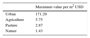
A detailed land use dataset for Tabasco was obtained through the Centro de Ciencias de la Atmósfera (Center for Atmospheric Sciences) of the Universidad Nacional Autónoma de México (UNAM). While the land use dataset describes 63 different land use classes, no detailed information was available on maximum damage per class, which is a required input for the flood damage estimations. Therefore, we aggregated the comprehensive dataset in four overarching categories with similar damage characteristics: Urban, Cultivation, Pastures, and Nature. To provide an estimate of damage, maximum damage values were obtained from the DamageScanner model (de Moel and Aerts, 2011; de Moel et al., 2014), converted into USD (2013), and corrected for the Mexican GDP (2013). These maximum damage values for Mexican land use categories are presented in Table II. For consistency with the flood hazard maps, we resampled the dataset to 30 arc seconds for calculating the EAD for river floods, and to 25×25 metres for calculating the EAD for coastal floods.
Additionally, to account for socio-economic growth, which increases the property values at risk over time, we corrected the maximum damage values for each year with the average annual projected GDP growth. We calculated the average annual GDP growth projection for different Socio-Economic Pathways (SSP) linked to the RCP2.6 and RCP8.5 pathways. Although in theory all SSPs can link to all RCPs, the SSP1-RCP2.6 SSP5-RCP8.5 combinations are often used in flood risk assessments because the greenhouse gas emission scenarios (RCPs) that underlie climate change projections are plausible combinations with these economic development pathways (SSPs) (Winsemius et al., 2016). The average annual GDP growth rate in both SSP1 and SSP5 is 3%, which we used to increase the maximum damage over time for the period 2010-2080.
3.1.3Depth-damage curvesThe relation between the inundation depth and the percentage of maximum damage is given by depth-damage curves (de Moel and Aerts, 2011; de Moel et al., 2014), which show for each land use class what percentage of the total value is damaged at a certain inundation depth. These curves are used to estimate the potential damage in Tabasco for each flood return period, using the aforementioned flood inundation depth and land use values as input. Depth-damage curves are used for flood risk assessments in many countries (de Moel et al., 2014), but currently there are, to our knowledge, no detailed depth-damage curves available for Mexico. Therefore, depth-damage curves from the DamageScanner model (Klijn et al., 2007) are used which are appli cable to estimating flood damages on the basis of the land use classes for Tabasco. For each aggregated land use class, the associated depth-damage curve is applied to calculate the damage as a percentage of the maximum value. According to the depth-damage curves, maximum damage is assumed to occur at a water depth of 5 metres.
3.2Cost-benefit analysis of flood adaptation strategiesUsing the EAD as input, we apply a CBA to determine whether flood protection by dike infrastructure is economically attractive, i.e. if the societal benefits of the project exceed the costs. To be economically attractive, the present value (PV) of the reduced expected annual damage (EADr), i.e. the reduction in flood risk of a strategy, should be higher than the PV of the investment and maintenance costs of building dike structures. Moreover, we estimate the economically optimal level of flood protection by the highest Net Present Value (NPV). The function for calculating the NPV is shown in equation 1.
Alternatively, results are presented as the benefit/ cost (B/C) ratio: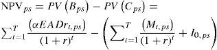
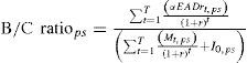
We calculate the NPV for different protection standards ps. The protection standards, which correspond to the flood return periods, for riverine protection are 5, 10, 25, 50, 100, 250, 500, and 1000 years. For coastal protection, the protection standards are 10, 100, and 1000 years. Benefits for each protection standard ps are represented by the sum of the EADr, for each time-step t, over the total dike lifespan of 100 years T. Benefits are time-dependent because flood risk changes due to climate change and socio-economic developments. The factor α represents the multiplier for indirect damages and is set to 1.6, in line with the average ratio in Table I (see supplementary material S1 for a sensitivity analysis).
Costs are calculated as the sum of maintenance costs Mt for the total dike length for each time-step t over the dike lifespan T, plus the initial investment costs I0 of the dike at t=0. Note that for river floods, the required dike height for each flood return period is calculated using the water volume for a certain return period, which implies that the dike should be high enough to keep the water volume for the given return period in the protected river channel. Furthermore, dike length and dike height are determined for each cell separately for both river and coastal dikes. For river dikes the dike length is two times the river length, as both riverbanks need to be protected. As there is often a floodplain between the river and the dike, to allow room for the river and to reduce the required dike height, it is assumed that the floodplain width is two times the current river width. In supplementary material S1 we show the sensitivity of the results to this parameter. Figure 5 shows the location of the envisaged dikes. The investment costs I0 applied here are 2.87 million USD/km length/metre height, and the maintenance costs Mt applied here are 0.08 million USD/km length. The investment costs were estimated as follows: the estimated costs for constructing dikes in the US (Bos, 2008) were converted to an estimate applicable to rural areas (i.e. to 1/3 of the normal cost), and by correcting it for construction costs differences between the US and Mexico, using an international construction price index, to 2010 values (Consultants Compass International, 2009). Maintenance costs were estimated by correcting estimates of dike maintenance costs in low- and middle-income countries (Mai et al., 2008) for differences in investment costs found for Mexico and those countries. The lifespan of the dike infrastructure is set at 100 years (Aerts and Botzen, 2011).
, and the modelled river one in 100-yr flood extent under current climate (blue). Right: Location of envisaged coastal flood protection infrastructure (red), and the modelled one in 100-yr coastal flood extent under current climate (blue).")
Left: Location of the envisaged river flood protection infrastructure (red), and the modelled river one in 100-yr flood extent under current climate (blue). Right: Location of envisaged coastal flood protection infrastructure (red), and the modelled one in 100-yr coastal flood extent under current climate (blue).
Future benefits and costs were discounted using a social discount rate r to reflect the opportunity costs of public capital. This discount rate is calculated following Ramsey's formula of the long-term discount rate, where r = ρ + θg. Here, ρ presents a rate of pure time preference, which we assume to be 1%, following Tol (2008). The average growth rate g is 3%, as calculated in Section 3.1.2, and the consumption elasticity of marginal utility θ is assumed to be 1. By applying Ramsey's formula, we obtain a baseline social discount rate of 4%. Supplementary material S1 shows the sensitivity of the results to using a higher social discount rate.
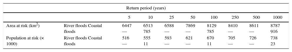
4Results4.1Flood riskAs shown by the flood extents in Figure 5, the modelled flood extent for river flooding is considerably larger than that of coastal flooding. Table III presents the modelled extent in km2 of different return periods for the state of Tabasco. While hurricanes are common in the Gulf of Mexico, they do not produce major storm surges along the coast of Tabasco (EHS-GA, 2008), and the modelled extent for coastal floods is thus relatively small (916 km2) compared with the areas that can be inundated by river flooding (8787 km2). Although hurricanes contribute to storm surges, their main impact in Tabasco is through heavy rainfall and consequent river flooding. This is aggravated due to deforestation in the upper catchment areas, a shallow topographical gradient, and poor flood management (EHS-GA, 2008). Table III shows that river floods can inundate a sizeable area of the state of Tabasco, between 6447 and 8787 km2. Table III furthermore shows the number of people under direct risk of flooding, by overlaying the inundation maps with a GRUMPv1 population density map (http://sedac. ciesin.columbia.edu/data/collection/grump-v1). These figures reflect the number of people located within the modelled flood zone. For river floods, the number of people at risk rises to 738 000 for a one in 1000-yr flood. In contrast, 23 000 people live in areas that can be inundated by the one in 1000-yr coastal flood. In reality, the number of people that are affected by either coastal or river floods can be far greater, as a consequence of damaged infrastructure and impeded access to livelihood needs. As an example, the 2007 Tabasco floods were reported to directly and indirectly affect 1 million people (EHS-GA, 2008). Note that the resampled elevation maps used to extrapolate coastal floods can only account for 1-metre differences. Since the surge heights for the one in 10-yr flood and 1 in 100-yr flood are within one metre of each other, the modelled area and population at risk are similar for both.
The area and population at risk of river flooding under current climate conditions.
| Return period (years) | |||||||||
|---|---|---|---|---|---|---|---|---|---|
| 5 | 10 | 25 | 50 | 100 | 250 | 500 | 1000 | ||
| Area at risk (km2) | River floods Coastal floods | 6447 — | 6513 785 | 6588 — | 7869 — | 8129 785 | 8410 — | 8611 — | 8787 916 |
| Population at risk (× 1000) | River floods Coastal floods | 516 — | 555 11 | 593 — | 621 — | 670 11 | 705 — | 726 — | 738 23 |
The difference in flood extents (and depths) of river and coastal floods also causes them to have significantly different impacts in terms of EAD. Table IV shows the EAD results for both coastal and river floods under different scenarios. For current climate, the model results show an EAD of 0.53 billion USD for coastal floods, and an EAD of 1.79 billion USD for river floods. While these values seem high, they are close to the reported damages in the period 2007-2011, when Tabasco was flooded (by river floods) on a yearly basis with a total damage of roughly five billion USD, as shown in Table I. This is equal to an average yearly damage of approximately one billion USD over this period, which is of the same order of magnitude as our model predictions.
Table IV shows that the EAD of river floods for Tabasco is approximately four times higher than the EAD for coastal floods, under the assumption of current climate conditions. In the low-SLR scenario, the EAD of coastal floods will rise to be six times higher in 2080 than under the assumption of a static sea level. The high-SLR scenario shows an only slightly higher EAD.
For river floods, the RCP2.6 scenario also results in a six times-higher EAD in the year 2080 compared with the results under a static climate assumption. Interestingly, the RCP8.5 scenario results in a lower EAD than the RCP2.6 scenario. While it is expected that global precipitation will increase with increased global mean temperature (IPCC, 2014), these changes are expected to exhibit substantial spatial variation; some regions will experience increases, while other regions will experience decreases or no significant changes at all. Although there is no specific data available for Tabasco, several models show that Mexico may on average experience drying (IDB, 2014). The two considered climate scenarios, which capture the range of extremes of a much wetter (RCP2.6) or slightly wetter climate (RCP8.5), provide a useful range for evaluating whether the CBA estimates of desirability of investments in flood protection are robust to this important source of uncertainty.
It is important to note that while the EAD is based on the simulated damages per return period, the value itself does not indicate that these damages will actually occur from year to year, due to the variability of flood disasters in practice. The EAD is instead specifically useful in CBA for determining economically efficient adaptation strategies, as it translates the uncertainty of low-probability flood events into yearly monetary terms (Eq. 1).
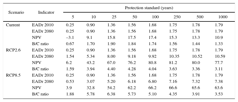
4.2CBA for riverine protection standardsTable V shows the CBA results for riverine protection standards in Tabasco. The current scenario shows the results for no change in climate conditions. This means that the EADr in 2010 for each protection standard is the same as the EADr in 2080. The results show that raising protection standards to withstand a flood with a return period of 10 years already reduces flood risk by half, and raising it to 25 years reduces it by an additional 25%. However, for the 5-yr protection standard, investment costs outweigh the benefits, as shown by the B/C ratio below 1. Even so, all other protection standards have B/C ratios above 1 and positive NPV values, which indicates that investing in dike structures is economically attractive. Furthermore, the results in Table V show that raising protection standards to 50 years yields the highest NPV, which indicates that this standard is the most economically desirable. In this case the B/C ratio is 1.84, meaning that every investment of one dollar will yield on average 1.84 dollars in benefits.
Results of CBA for different river flood protection standards, for different scenarios of climate conditions. The EADr and NPV are shown in billion USD.
| Scenario | Indicator | Protection standard (years) | |||||||
|---|---|---|---|---|---|---|---|---|---|
| 5 | 10 | 25 | 50 | 100 | 250 | 500 | 1000 | ||
| Current | EADr 2010 | 0.25 | 0.90 | 1.36 | 1.56 | 1.68 | 1.75 | 1.78 | 1.79 |
| EADr 2080 | 0.25 | 0.90 | 1.36 | 1.56 | 1.68 | 1.75 | 1.78 | 1.79 | |
| NPV | –3.1 | 9.1 | 15.8 | 17.5 | 17.4 | 15.3 | 13.3 | 10.9 | |
| B/C ratio | 0.67 | 1.70 | 1.90 | 1.84 | 1.74 | 1.56 | 1.44 | 1.33 | |
| RCP2.6 | EADr 2010 | 0.25 | 0.90 | 1.36 | 1.56 | 1.68 | 1.75 | 1.78 | 1.79 |
| EADr 2080 | 1.54 | 5.34 | 8.00 | 9.18 | 9.92 | 10.35 | 10.52 | 10.59 | |
| NPV | 6.2 | 43.2 | 67.0 | 76.2 | 80.8 | 81.2 | 80.0 | 77.7 | |
| B/C ratio | 1.59 | 3.94 | 4.40 | 4.28 | 4.04 | 3.63 | 3.36 | 3.11 | |
| RCP8.5 | EADr 2010 | 0.25 | 0.90 | 1.36 | 1.56 | 1.68 | 1.75 | 1.78 | 1.79 |
| EADr 2080 | 0.53 | 3.07 | 5.20 | 6.18 | 6.80 | 7.16 | 7.32 | 7.38 | |
| NPV | 3.9 | 32.8 | 54.2 | 62.2 | 66.2 | 66.6 | 65.6 | 63.6 | |
| B/C ratio | 1.88 | 5.78 | 6.38 | 5.73 | 5.10 | 4.35 | 3.91 | 3.53 | |
Because the assumption of static flooding conditions is unlikely considering climate change, the CBA results are also presented for climate change under RCP2.6 and RCP8.5 scenarios in Table V. The slightly wetter climate projected under scenario RCP8.5, in comparison to current climate conditions, leads to a lower EAD reduction in 2080 than the RCP2.6 scenario. As a result, the NPV for each protection standard are lower for the RCP8.5 scenario than they are under the RCP2.6 scenario. Nevertheless, Table V shows that increasing riverine protection standards is economically desirable for all protection standards under future climate conditions. Moreover, NPV values are roughly up to seven and six times higher under the RCP2.6 and RCP8.5 scenarios respectively, than under the assumption of no climate change. The results for the RCP2.6 and RCP8.5 scenarios show that the NPV is highest for the 250-yr protection standard, with each dollar invested yielding on average 3.63 and 4.35 dollars for the RCP2.6 and RCP8.5 scenarios, respectively. Moreover, the results for the climate change scenarios again show a significant reduction in the EAD for the protection standards of 10 and 25 years, indicating that there is much to gain from relatively small investments.
It is important to note that while both climate change scenarios return the same optimum protection level of 250 years, the actual height to build the flood protection infrastructure differs for each scenario. A 250-yr protection standard under the RCP2.6 scenario indicates higher dike heights than under the RCP8.5 scenario.
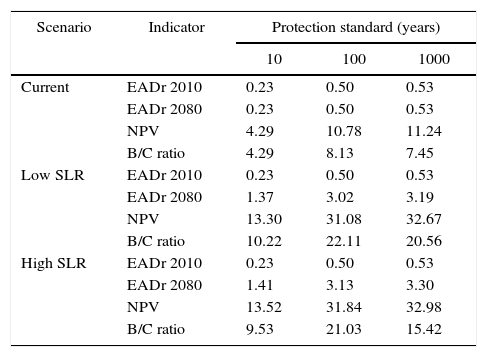
4.3CBA for coastal protection standardsTable VI presents the CBA results for different protection standards for coastal flooding, under different assumptions of climate change. Since the EAD is significantly smaller than for river floods, so too is the EAD that can be reduced by increasing coastal protection standards. However, as shown by Figure 5, the total length of the dikes is also significantly lower, and therefore so are investment costs. The results for the current climate conditions show that a 10-yr coastal protection standard reduces the EAD by about 1/3, while a 100-yr protection standard reduces the EAD by a little over 90%. Raising protection standards from 100 to 1000 years does not significantly reduce EAD. As a result of the relatively low investment costs, B/C ratios are in general higher than for riverine protection, under the similar assumption of static climate conditions. For coastal protection standards, each dollar invested would yield 4.29, 8.13, and 7.45 for the 10-, 100-, and 1000-yr standards, respectively. The NPV is highest for raising protection standards to 1000-yrs, although it is close to the NPV of protecting against the one in 100-yr flood.
Results of CBA for different coastal protection standards under different scenarios. The EADr and NPV are shown in billion USD.
| Scenario | Indicator | Protection standard (years) | ||
|---|---|---|---|---|
| 10 | 100 | 1000 | ||
| Current | EADr 2010 | 0.23 | 0.50 | 0.53 |
| EADr 2080 | 0.23 | 0.50 | 0.53 | |
| NPV | 4.29 | 10.78 | 11.24 | |
| B/C ratio | 4.29 | 8.13 | 7.45 | |
| Low SLR | EADr 2010 | 0.23 | 0.50 | 0.53 |
| EADr 2080 | 1.37 | 3.02 | 3.19 | |
| NPV | 13.30 | 31.08 | 32.67 | |
| B/C ratio | 10.22 | 22.11 | 20.56 | |
| High SLR | EADr 2010 | 0.23 | 0.50 | 0.53 |
| EADr 2080 | 1.41 | 3.13 | 3.30 | |
| NPV | 13.52 | 31.84 | 32.98 | |
| B/C ratio | 9.53 | 21.03 | 15.42 | |
While it is already economically attractive to raise coastal protection standards in Tabasco under current climate conditions, it becomes increasingly attractive if SLR is included. Table VI also presents the CBA results for the low-SLR and high-SLR scenarios. The differences between the SLR scenarios are small, and the NPV of flood protection is slightly higher under the high-SLR scenario compared with the low-SLR scenario. Under both climate change scenarios, it would be economically rational to raise protection standards. Raising protection standards to 1000 years yields the highest NPV for both scenarios, with B/C ratios of 20.56 dollars for each invested dollar in the low-SLR scenario, and 15.42 dollars for each invested dollar in the high-SLR scenario. These values are higher than the riverine protection standards, and, considering the high percentage of EADr, there are substantial benefits of implementing coastal protection standards. Note that for coastal protection, the 10-, 100- and 1000-yr protection standards were assessed. Although it was found that a 1000-yr protection standard yields a higher NPV than the 100-yr protection standard, the optimum value is likely to lie somewhere in-between. Consequently, it is considered economically optimal to have a protection standard of at least 100 years.
Similarly to river floods, a 1000-yr protection standard for the low-SLR scenario implies a lower dike structure compared to the same protection standard for the high-SLR scenario. Considering the approximately similar NPV and B/C values for both scenarios, the safe policy strategy could be to follow the high-SLR scenario in the design of flood protection infrastructure.
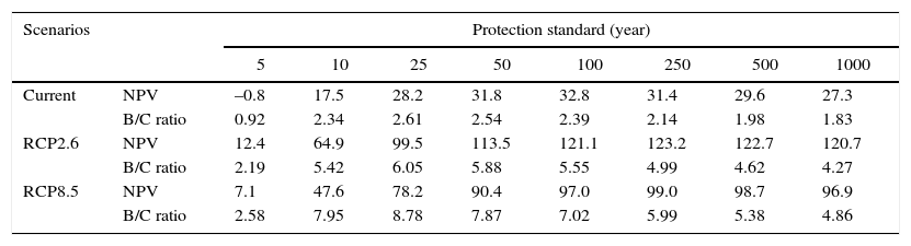
4.4Sensitivity of main results to key assumptionsAn important source of uncertainty is the indirect damage, i.e. business interruption, caused by floods. The results in Section 4.3 are based on the assumption that indirect damage is 60% of direct damage (α = 1.6), the average factor in Table I. To test the sensitivity of the results, we set the α to both half the size of the initial assumption of indirect damage respective to direct damage (30%) and double the size (120%), therefore to factors of 1.3 and 2.2, respectively. As can be expected, NPV values become lower if α is set to 1.3, and NPV values become higher if α is set to 2.2 (Tables SI-SIV in the supplementary material). When α is set to 1.3, if no climate change is assumed, the optimal protection standard for the large-scale protection of rivers envisaged in Figure 5 remains a 50-yr protection standard. However when climate change is taken into account, we find that the optimal protection standard for rivers is 100 years instead of 250 years. For an α of 2.2, the current climate optimum changes to a 100-yr protection standard, and for future climate the 250-yr protection standard remains optimal. The 1000-yr protection standard is optimal for the coast under all assumptions, although as previously noted, it is more likely to be between the 100-yr and 1000-yr coastal protection assessed here.
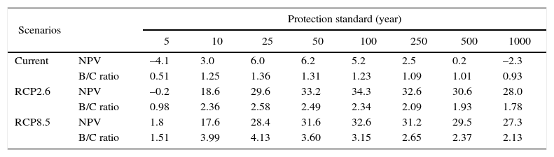
Furthermore, different assumptions about the discount rate used for translating future monetary costs and benefits to current values in the CBA indicators may influence these conclusions. We assumed that the rate of pure time preference ρ is 1%, leading to a baseline value for the social discount rate r of 4%. However, a higher bound rate of pure time preference of 3% has been assumed in other studies (e.g., see Tol, 2008). Therefore, the social discount rate was set to 6% to test the sensitivity of our results to this higher value. As a result, all NPV and B/C ratios become lower (Tables SV-SVI in the supplementary material). With a social discount rate of 6%, we find that a 50-yr protection standard is optimal under the assumption of current climate conditions. Under future climate conditions, the economic optimum remains a 250-yr protection standard. The 5-yr protection standard now has a negative NPV under the RCP2.6 scenario, and is therefore economically undesirable. The conclusions for coastal protection remain the same, although with lower NPV and B/C ratios.
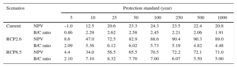
Finally, we assumed for riverine protection standards that there is a floodplain that is twice the width of the river channel. This is a common strategy to allow space for the river and decrease the required height for dikes. However, it is preferable to allow even more room for the river if space allows, reducing the needed dike height. As Tabasco is a mostly rural area, it is probably possible to allow more room for the river, and therefore we tested the sensitivity by setting the floodplain width to three times the river channel width. Table SVII in the supplementary material shows that for future climate, the 250-yr protection standard would remain economically optimal.
5Discussion and conclusionsThis study has illustrated how a multi-disciplinary approach of hazard modelling, natural disaster risk assessment, and economic cost-benefit analysis (CBA) of risk management options, can guide investments by policy-makers in adaptation measures, that are robust under a variety of future climate conditions. In particular, our analyses focusing on river and coastal flood risk in the Mexican state of Tabasco showed that installing flood protection infrastructure appears to be economically desirable. Tabasco is exposed to almost yearly flood events that cause substantial damage, and the results of CBA indicate that the costs involved in preventing these flood disasters pay off in the long term in terms of prevented flood damages.
Notably, we find that a 100- or 250-yr protection standard for dikes on the main rivers of Tabasco is economically optimal, for different assumptions, if climate change is taken into account. This means that dikes should be designed to be strong and high enough to withstand a flood event that occurs on average once in 100 or once in 250 years. The optimality of the 100-yr protection standard is robust to different future climate conditions, which imply either a slightly or much wetter climate, as well as key uncertainties about indirect damages (i.e. business interruption) of floods, discounting of future values in the CBA, and the planned width of the river channel. Moreover, our coastal analyses showed that coastal protection with a safety standard that protects against at least a one in 100-yr storm surge, or even stronger storms, is economically optimal under a variety of sensitivity analyses. Although the results presented here show that a 1000-yr coastal protection standard is more economically desirable than a 100-yr standard, care should be taken in interpreting this result since we were not able to examine the optimality of intermediate standards, such as 250-yr or 500-yr standards. Nevertheless, it is clear from our findings that having a coastal safety standard that protects against the one in 100-yr storm and beyond could greatly reduce risk. The approach in this paper was conducted on an aggregated geographical level, which provides insights into whether policy-makers should consider planning for flood protection in Tabasco, and what safety standard for the river basin and coastline should be considered in this planning process.
Future research should aim at creating improved local models or obtaining better local information to determine what kind of flood protection infrastructure is the most suitable for specific areas in Tabasco, since a single solution can rarely be applied to an entire basin. The current flood risk analysis could be improved by developing hydrological models of the local rivers in Tabasco that also account for local dam management practices. Such increasingly refined hydrological models can be used to simulate flooding conditions using geographically detailed elevation maps, which can produce more refined flood inundation maps than those presented here. Additionally, flood risk may be exacerbated by land subsidence in Tabasco, for which currently no data are available. Since land subsidence can have a major influence on coastal flood risk (Haer et al., 2013), this needs to be examined in future research. Furthermore, the framework was also presented for one General Circulation Model (CGM); HadGEM2-ES. As different GCMs can result in different climate projections (Sperna-Weiland et al., 2012), future research should integrate more GCMs to reduce this uncertainty. Moreover, while we examined river and coastal flooding separately, future research could examine flood risk under compound events. This joint modelling of coastal and river floods is relevant for capturing situations when high precipitation and consequent river discharge coincide with a storm surge along the coast, or when river discharge to the ocean is hampered by a risen sea-level (Aparicio et al., 2009). New time series of surge and tide levels at the global scale (Muis et al., 2016) enable developing research in this area.
Damage assessment can be improved with local information on potential damage for a larger variety of land use classes. Moreover, depth-damage curves, which are calibrated using Mexican data of experienced flood losses in relation to observed flood hazard conditions, could further improve the analysis. This requires the systematic collection of data about local damages, hazards, and exposure conditions, which can be performed using surveys following flood events. Our more aggregated approach presented here can be adapted for such local analyses, because the basic setup of the modelling approaches presented can be applied on a local scale, as is shown, for example, for a city-scale study in Aerts et al. (2014).
Despite the aggregated nature of the methods presented here, the model estimates of potential flood damages are close to damages observed during past flood events, and the great benefits of flood protection provide confidence in the economic efficiency of these measures. Nevertheless, it should be realised that large engineering structures could have negative side-effects, such as the levee effect and technical lock-in. Adaptation strategies therefore need to extend beyond flood protection infrastructure. For example, potential flood damages can be reduced by limiting urban expansion in natural floodplains, and buildings can be improved to enable them to better withstand impacts from floods, rain, and wind. Improved early warning and forecasting systems and evacuation planning can help to minimise casualties during flood events. The desirability and implementation of these alternative flood risk management measures can also be guided by studies of local flood risk analyses and CBA of investing in these measures, for which we hope our study provides a useful starting point.
This research was partly funded by the Zurich Flood Resilience Program. PJW received additional funding from the Netherlands Organisation for Scientific Research (VIDI grant: 016.161.324).
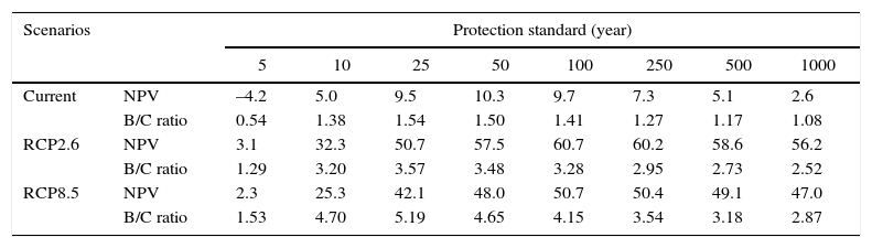
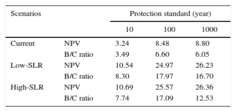
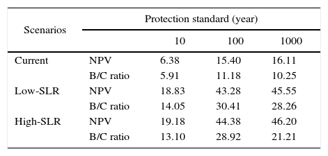
In this study, we assume that the multiplier for indirect damages α is 1.6, i.e. indirect damage is 60% the size of direct damage. Table SI shows the CBA results for an α of 1.3 (indirect damage = 30% the size of direct damage) and Table SII shows the results for an α of 2.2 (indirect damage = 120% the size of direct damage) for river floods. Lowering α consequently lowers the NPV and B/C ratios. Under static current climate conditions, the 50-yr return period would remain the optimal investment. When taking into account future climate conditions, the optimum shifts to a 100-yr protection standard when α = 1.3. For increasing α to 2.2, we find higher NPV and B/C ratios. Moreover, under the current climate, the 100-yr protection standards is the new optimal investment, and under the future climate, the 250-yr protection standard remains optimal. The conclusions for coastal protection, shown in Tables SIII and SIV, remain the same as for an α of 1.6.
NPV and B/C ratios for α = 1.3 for different riverine protection standards, assuming current climate conditions. EAD and NPV are shown in billion USD.
| Scenarios | Protection standard (year) | ||||||||
|---|---|---|---|---|---|---|---|---|---|
| 5 | 10 | 25 | 50 | 100 | 250 | 500 | 1000 | ||
| Current | NPV | –4.2 | 5.0 | 9.5 | 10.3 | 9.7 | 7.3 | 5.1 | 2.6 |
| B/C ratio | 0.54 | 1.38 | 1.54 | 1.50 | 1.41 | 1.27 | 1.17 | 1.08 | |
| RCP2.6 | NPV | 3.1 | 32.3 | 50.7 | 57.5 | 60.7 | 60.2 | 58.6 | 56.2 |
| B/C ratio | 1.29 | 3.20 | 3.57 | 3.48 | 3.28 | 2.95 | 2.73 | 2.52 | |
| RCP8.5 | NPV | 2.3 | 25.3 | 42.1 | 48.0 | 50.7 | 50.4 | 49.1 | 47.0 |
| B/C ratio | 1.53 | 4.70 | 5.19 | 4.65 | 4.15 | 3.54 | 3.18 | 2.87 | |
NPV and B/C ratios for α = 2.2 for different riverine protection standards, assuming current climate conditions. EAD and NPV are shown in billion USD.
| Scenarios | Protection standard (year) | ||||||||
|---|---|---|---|---|---|---|---|---|---|
| 5 | 10 | 25 | 50 | 100 | 250 | 500 | 1000 | ||
| Current | NPV | –0.8 | 17.5 | 28.2 | 31.8 | 32.8 | 31.4 | 29.6 | 27.3 |
| B/C ratio | 0.92 | 2.34 | 2.61 | 2.54 | 2.39 | 2.14 | 1.98 | 1.83 | |
| RCP2.6 | NPV | 12.4 | 64.9 | 99.5 | 113.5 | 121.1 | 123.2 | 122.7 | 120.7 |
| B/C ratio | 2.19 | 5.42 | 6.05 | 5.88 | 5.55 | 4.99 | 4.62 | 4.27 | |
| RCP8.5 | NPV | 7.1 | 47.6 | 78.2 | 90.4 | 97.0 | 99.0 | 98.7 | 96.9 |
| B/C ratio | 2.58 | 7.95 | 8.78 | 7.87 | 7.02 | 5.99 | 5.38 | 4.86 | |
NPV and B/C ratios for α = 1.3 for different coastal protection standards, assuming current climate conditions. EAD and NPV are shown in billion USD.
| Scenarios | Protection standard (year) | |||
|---|---|---|---|---|
| 10 | 100 | 1000 | ||
| Current | NPV | 3.24 | 8.48 | 8.80 |
| B/C ratio | 3.49 | 6.60 | 6.05 | |
| Low-SLR | NPV | 10.54 | 24.97 | 26.23 |
| B/C ratio | 8.30 | 17.97 | 16.70 | |
| High-SLR | NPV | 10.69 | 25.57 | 26.36 |
| B/C ratio | 7.74 | 17.09 | 12.53 | |
NPV and B/C ratios for α = 2.2 for different coastal protection standards, assuming current climate conditions. EAD and NPV are shown in billion USD.
| Scenarios | Protection standard (year) | |||
|---|---|---|---|---|
| 10 | 100 | 1000 | ||
| Current | NPV | 6.38 | 15.40 | 16.11 |
| B/C ratio | 5.91 | 11.18 | 10.25 | |
| Low-SLR | NPV | 18.83 | 43.28 | 45.55 |
| B/C ratio | 14.05 | 30.41 | 28.26 | |
| High-SLR | NPV | 19.18 | 44.38 | 46.20 |
| B/C ratio | 13.10 | 28.92 | 21.21 | |
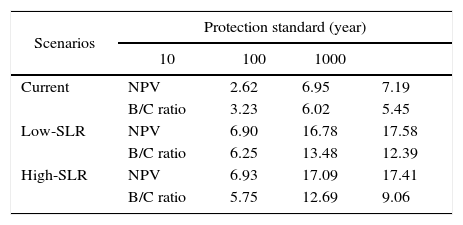
For the social discount rate r, we assumed that the rate of pure time preference ρ is 1%, following Tol (2008), leading to a social discount rate of 4% based on the Ramsey's formula. However, Tol (2008) also indicates that some studies use a rate of pure time preference of 3%. Therefore, we changed the social discount rate to 6% here. The results are shown in Table SV for river floods and Table SVI for coastal floods. All NPV and B/C ratios are lower. If it is assumed that the climate does not change, optimal river protection standards remain at 50 year at an r of 6%. Furthermore, the 5-yr protection standard under the RCP2.6 scenario is no longer economically desirable. Both RCP2.6 and RCP8.5 scenarios now result in a highest NPV for a protection standard of 100 years. All conclusions for the coastal protection standards remain the same, but with lower NPV and B/C ratios, as shown in Table SVI.
NPV and B/C ratios for r = 6% for different riverine protection standards, assuming current climate conditions. EAD and NPV are shown in billion USD.
| Scenarios | Protection standard (year) | ||||||||
|---|---|---|---|---|---|---|---|---|---|
| 5 | 10 | 25 | 50 | 100 | 250 | 500 | 1000 | ||
| Current | NPV | –4.1 | 3.0 | 6.0 | 6.2 | 5.2 | 2.5 | 0.2 | –2.3 |
| B/C ratio | 0.51 | 1.25 | 1.36 | 1.31 | 1.23 | 1.09 | 1.01 | 0.93 | |
| RCP2.6 | NPV | –0.2 | 18.6 | 29.6 | 33.2 | 34.3 | 32.6 | 30.6 | 28.0 |
| B/C ratio | 0.98 | 2.36 | 2.58 | 2.49 | 2.34 | 2.09 | 1.93 | 1.78 | |
| RCP8.5 | NPV | 1.8 | 17.6 | 28.4 | 31.6 | 32.6 | 31.2 | 29.5 | 27.3 |
| B/C ratio | 1.51 | 3.99 | 4.13 | 3.60 | 3.15 | 2.65 | 2.37 | 2.13 | |
NPV and B/C ratios for r = 6% for different coastal protection standards, assuming current climate conditions. EAD and NPV are shown in billion USD.
| Scenarios | Protection standard (year) | |||
|---|---|---|---|---|
| 10 | 100 | 1000 | ||
| Current | NPV | 2.62 | 6.95 | 7.19 |
| B/C ratio | 3.23 | 6.02 | 5.45 | |
| Low-SLR | NPV | 6.90 | 16.78 | 17.58 |
| B/C ratio | 6.25 | 13.48 | 12.39 | |
| High-SLR | NPV | 6.93 | 17.09 | 17.41 |
| B/C ratio | 5.75 | 12.69 | 9.06 | |
NPV and B/C ratios for a flood plain two third of the river channel width, for different riverine protection standards, assuming current climate conditions. EAD and NPV are shown in billion USD.
| Scenarios | Protection standard (year) | ||||||||
|---|---|---|---|---|---|---|---|---|---|
| 5 | 10 | 25 | 50 | 100 | 250 | 500 | 1000 | ||
| Current | NPV | –1.0 | 12.5 | 20.6 | 23.3 | 24.3 | 23.5 | 22.4 | 20.8 |
| B/C ratio | 0.86 | 2.29 | 2.62 | 2.58 | 2.45 | 2.21 | 2.06 | 1.91 | |
| RCP2.6 | NPV | 8.6 | 47.0 | 72.5 | 82.9 | 88.6 | 90.4 | 90.3 | 89.0 |
| B/C ratio | 2.09 | 5.36 | 6.12 | 6.02 | 5.73 | 5.19 | 4.82 | 4.48 | |
| RCP8.5 | NPV | 4.4 | 34.0 | 56.5 | 65.5 | 70.5 | 72.2 | 72.1 | 71.0 |
| B/C ratio | 2.10 | 7.10 | 8.32 | 7.70 | 7.00 | 6.07 | 5.50 | 5.00 | |
The height of the dikes for river protection is calculated based on the total flood volume remaining within the floodplain w, which is twice the channel width. As shown in Figure S1, this leads to a water height h. If possible, e.g. if the dikes are not located in urban areas, more tolerance of flood plain width is preferable to allow more room for the river, and to reduces the required dike-height. As the Tabasco rivers flow mainly through rural areas, we test the sensitivity by increasing the floodplain to three times the channel width. Since Tabasco is relatively flat, this means that dike heights are two third the height that would be required if the dikes were located directly on the river banks, as illustrated in Figure S1. Table SVII shows the results where we allow for a flood plain of triple the channel width. The economic optimum under an assumption of current climate is now a 100-yr protection standard. Under future climate conditions, the economic optimum remains a 250-yr protection standard.
