A Lagrangian PFEM approach for non-Newtonian viscoplastic materials

Abstract

This paper presents the application of a stabilized mixed Particle Finite Element Method (PFEM) to the solution of viscoplastic non-Newtonian flows. The application of the proposed model to the deformation of granular non-cohesive material is analysed. A variable yield threshold modified Bingham model is presented, using a Mohr Coulomb resistance criterion.

Since the granular material is expected to undergo severe deformation, a Lagrangian approach is preferred to a fixed mesh one. PFEM is the adopted technique.

The detail of the discretization procedure is presented and the Algebraic Sub-Grid Scale (ASGS) stabilization technique is introduced to allow for the use of equal order interpolations for velocity and pressure in a consistent way. The matrix form of the problem is given.

Finally, the differences between the regularized Bingham and the variable yield models are discussed in some examples.

1

Introduction

In the present work, the simulation of the structural response of a slope made of dry granular non cohesive material (rockfill-like) has been treated using a continuous approach. This is an acceptable choice under the assumption that the rockfill size is small with respect to the overall size of the structure.

Nevertheless it should be mentioned that in recent years, the great advance in computer performance and in parallel computing has allowed the simulation of the mechanical behaviour of every single particle of a granular slope. The family of the so called Discrete (or distinct) Element Methods (DEM) has been reaching a widespread popularity in the computational mechanics community. The basic idea is that every particle is a discrete element interacting with the others considering its mechanical and material properties. The problem is that commonly spherical or ellipsoidal particles are used and therefore ah hoc calibration of contacts forces should be performed so to reproduce correctly the effects of the non-spherical real shape and roughness of the particle. Multi scale approaches are often needed to correctly reproduce the macroscopic behaviour.

The adoption of a continuous approach leads to the choice of a suitable constitutive law. Many plastic or rigid-plastic constitutive models are commonly used in geomechanics to describe the structural response of an incoherent non-cohesive material, like roskfill. It is usually accepted that a rockfill slope has the capability to support a certain amount of shear stress with negligible elastic strain, before starting large deformation. When the yield stress is reached, the material starts to flow until arriving to a stable configuration. It should be noted that the behaviour of the yielded material is more similar to a fluid than to the process of deformation of a solid. In the literature there exists a wide category of fluids which exhibits a rigid behaviour till reaching a yield threshold. These are the so-called non-Newtonian viscoplastic fluids.

These aspects, together with the natural way of managing large deformations in fluids, lead us to concentrate on variable viscosity models. Consequently, a non-Newtonian constitutive law has been adopted for the rockfill body. This implies that the rockfill stiffness is controlled by very high values of the viscosity. Only when the yield threshold is exceeded, the viscosity dramatically decreases and the material starts flowing. When the material stops its motion, the viscosity recovers its initial values for which the stress level does not exceed the yield limit.

The model developed in this work has its origin in the traditional Bingham plastics using the regularization proposed by Papanastasiou to overcome numerical problems induced by the bilinear stress-strain curve [1]. Nevertheless in order to include a Mohr-Coulomb failure criteria (without cohesion), the possibility of considering a variable yield level is also introduced.

The two constitutive models with constant and variable yield, are presented at the beginning of the present work after a brief overview on non-Newtonian models.

The equations governing the structural problem are studied in their weak form arriving to the algebraic solution system which is solved with a fully implicit scheme. A stabilized, equal-order, mixed velocity-pressure element technology is chosen so to guarantee a locking free behavior [2–4].

Since the structural domain is expected to undergo severe deformation as the failure progresses, the kinematic model has to adapt dynamically to such deformations. The Particle Finite Element Method (PFEM) provides the necessary flexibility with a powerful remeshing mechanism [5,6]. Its features are described in the second part of this paper.

In the last part of the paper some examples are inserted to validate the Bingham model and to appreciate its differences with respect to the proposed variable viscosity approach. Finally the dambreak of granular slopes with different frictional angles is simulated to verify that the model correctly reproduces the expected mechanical properties.

2

Governing equations

The problem of incompressible isothermal flow is defined by the Navier-Stokes equations.

Calling Ω⊂ℝd (where d is the space dimension) the material domain in a time interval (0, T), the Navier-Stokes equations are

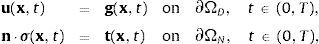
where σ is the Cauchy stress tensor, u is the velocity, ρ is the density and b is the volumetric force. The problem is fully defined with the following boundary conditions:

where Ω_D and Ω_N are Dirichlet and Neumann boundary respectively.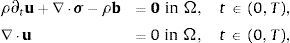

The presented model has been developed in a Lagrangian framework, hence, the convective term is not present in Eq. (1).

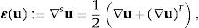
The stress tensor (σ) of Eq. (1) can be decomposed in its volumetric and deviatoric parts as follow

where p is the pressure, τ is the devatoric stress which can also be expressed as a function of the dynamic viscosity μ times the strain tensor ¿, which is, by definition,

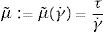
Fluids for which the relations between τ and ¿(u) is not constant, are called non-Newtonian. In this case viscosity cannot be considered as a property of the material as it is strictly dependent on the deformation process. This classification is very general and includes a wide range of different constitutive relations. Let us consider a 1D problem and let us define an apparent viscosityμ˜ like the ratio between the shear stress τ and the shear rate γ˙

Among the possible families of non Newtonian fluids, in this work we will take into consideration the viscoplastic ones. These are characterized by the existence of a threshold stress, the yield stress, which must be exceeded for the fluid to deform. For lower values of stress the visco-plastic fluids are completely rigid, or show some sort of elasticity. Once the yield stress is reached and exceeded, they can exhibit a Newtonian-like behavior with a constant apparent viscosity (Bingham plastics fluids) or showing a shear thinning behavior (yield-pseudoplastic fluids).

A deep analysis of non-Newtonian fluids behavior falls outside the scope of this work. For a comprehensive review of the topic see [7–9].

2.1

Constant yield: the Bingham model

Bingham fluids were first described by Eugene C. Bingham in 1919. While analyzing the constitutive behaviour of paints, he discovered that such fluids exhibit a negligible deformation till reaching a threshold: the yield stress. When this stress limit is exceeded, they behave like a Newtonian fluid. According to Papanastasiou [1] a wide range of materials have been identified to have a yield threshold. Bird [10] was the first to give a lists of several Bingham plastics, most of these products came from food or chemical industry. Among them we can list, for instance, slurries, pastes, or food substances like margarine, ketchup, mayonnaise and others.

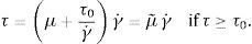
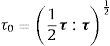
The 1D constitutive relation for a Bingham plastic can be defined as follows. Calling τ₀ the yield stress

where γ˙ is the rate of strain, μ is the dynamic viscosity and τ the shear stress.

Eq. (6b) can be rewritten as

Special care should be taken in Eq. (7) when the level of stress is lower than the yield stress. In this case, according to Eq. (5), the apparent viscosity approaches infinity, i.e. μ˜→∞ as γ˙→0. Since this behavior might induce numerical difficulties, regularized models are usually preferred. Different procedures are proposed in the literature to deal with the discontinuity problem. The nonlinear problem can be rewritten in the form of a variational inequality model, following the original work by Duvaut and Lions [11]. It can be demonstrated [12] that the solution of the constrained variational inequality is equivalent to a minimization problem of an equivalent variational equality form. Alternatively a regularization of the constitutive law can be employed [1]. This second approach has been used in this work. The main reason for regularizing the discontinuity of the exact viscoplastic behaviour is to allow its direct implementation in standard numerical solvers.

Following the ideas presented in [1], Eq. (7) is regularized using Papanastasou model, as follow

where m is a regularization parameter that controls the approximation to the bilinear model as shown in Fig. 1.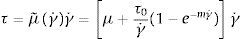

Fig. 1.

Newtonian and Bingham fluid compared with the regularized model for increasing values of the m parameter.

The problems connected with the singular point of the bi-linear model are here avoided. Since the shear strain rate μ˜=μ+τ0   m as γ˙→0.

In order to introduce the constitutive model for 3D problems, the following equivalent strain rateγ˙ and yield stress τ₀ are defined as the second invariants of the rate of strain tensor (¿) and of the deviatoric part of the stress tensor (τ), respectively

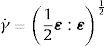
Eq. (8), for 3D problems, becomes

where μ˜B is the apparent viscosity for the 3D reguralized Bingham model.

2.2

Variable yield visco-rigid model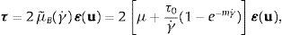

The Bingham model presented in the previous section was conceived for materials with a fixed yield stress.

For granular materials, the definition of the yield stress depends on:

• -

  The characteristics of the rockfill (its internal friction angle).

• -

  The presence of water inside the grains. It acts decreasing the effective stress leading to a significant loss of resistance.

The model proposed in the present work has its origin in a classical Bingham constitutive relation but the yield stress τ₀ is not constant any more. τ₀ is pressure sensitive and it is defined using a Mohr-Coulomb failure criteria without cohesion

where p is the pressure and ϕ is the internal friction angle.

In this case, Eq. (8), in 3D, becomes

where μ˜V(γ˙) is the apparent viscosity of the variable yield regularized model.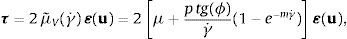

The idea of a pressure dependent yield stress has already been exploited for instance in [13,14], where a frictional fluid rehological model is used for the simulation of landslides.

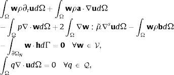
3

Weak form

Using the Galerkin formulation the weak form of the general problem becomes

where, for a fixed t ∈ (0, T), u is assumed to belong to the velocity space V∈[H1(Ω)]d of vector functions whose components and their 1st derivatives are square-integrable, and p belongs to the pressure space Q∈L2 of square-integrable functions. w and q are velocity and pressure weight functions belonging to velocity and pressure spaces respectively.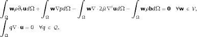

Performing the integration by parts of the pressure and the viscous terms and inserting the boundary conditions (Eqs. (2)), gives

Let Vh be a finite element space to approximate V, and Qh a finite element approximation to Q. The problem is now finding uh∈Vh and ph∈Qh such that

4

The monolithic solution strategy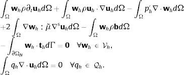

In the following sections the procedure used for obtaining the algebraic stabilized system of equations, the time integration scheme and the solution strategy are briefly described.

In order to obtain the final solution system, the weak form represented by Eqs. (16) have to be stabilized and linearized in time. Finally a quasi-Newton residual based strategy is adopted to solve the non linear problem.

4.1

Stabilized formulation

The choice of adopting equal order linear elements for velocity and pressure, despite of the simplicity, entails the necessity of using a stabilization technique. An ASGS stabilization technique is employed for that purpose. The derivation of the stabilization scheme is analogous to what has been presented in [4,15]. Therefore, in what follows, only the final stabilized form and the stabilization terms is reported.

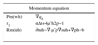
The stabilized form of the balance equations becomes

where Psm, Rsm, Psc and Rsc are defined in Table 1.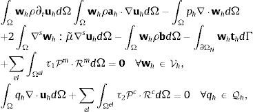

Table 1.

Stabilizing elemental terms in ASGS for the non-Newtonian element.

Momentum equation
Pm(wh)	∇qh
τ1	αΔt+4μ˜h2ρ−1
Rm(uh)	∂tuh−∇·μ˜ρ∇suh+∇ph−b

Continuity equation
Pc(wh)	∇ · wh
τ2	μ˜ρ
Rc(uh)	∇ · uh

In a Lagrangian framework the convective term is not present. Therefore only pressure stabilization is required.

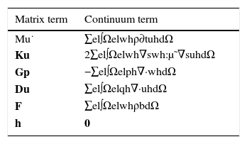
4.2

Discretization procedure

The matrix form of the stabilized system of Eqs. (17) can be written as:

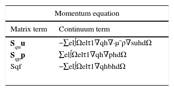
where the operators are explicitly written in Table 2 and the stabilization operators can be found in Table 3.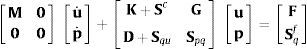

Table 2.

Matrices and vectors of system (18) without stabilization terms.

Matrix term	Continuum term
Mu˙	∑el∫Ωelwhρ∂tuhdΩ
Ku	2∑el∫Ωelwh∇swh:μ˜∇suhdΩ
Gp	−∑el∫Ωelph∇·whdΩ
Du	∑el∫Ωelqh∇·uhdΩ
F	∑el∫ΩelwhρbdΩ
h	0

Table 3.

Stabilization matrices and vectors of system (18).

Momentum equation
Matrix term	Continuum term
Squu	−∑el∫Ωelτ1∇qh∇·μ˜ρ∇suhdΩ
Sqpp	∑el∫Ωelτ1∇qh∇phdΩ
Sqf	−∑el∫Ωelτ1∇qhbhdΩ

Continuity equation
S^cu	∑el∫Ωelτ2∇·wh∇·uhdΩ

4.3

Bossak time integration scheme

A Bossak time integration scheme is used to discretize in time the momentum equations.

Eq. (18) can be written in compact form as

The resulting residual of the momentum equations linearized in time is

where v^T = [u, p] and v˙T=[u˙,p˙] are the vectors of unknowns. The super indices n and n + 1 indicate the current (known) and next (unknown) time steps respectively. α_B and δ are the parameters of the scheme.

4.3.1

Predictor multi corrector residual based strategy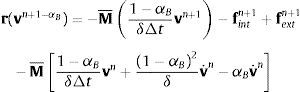

A predictor multi corrector strategy is adopted. The linearization of the non-linear terms is performed using a quasi Newton method.

The viscous terms is the non linear part of the balance equations. When calculating the LHS, this is linearized as follows

being k the iteration counter.

5

Kinematic framework: the Particle Finite Element Method (PFEM)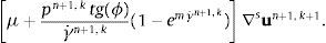

Since the structural domain is expected to undergo severe deformations, the kinematic model has to adapt dynamically to such deformations leading to the preferable choice of a Lagrangian approach. Among many possible Lagrangian methods, the Particle Finite Element Method (PFEM) has been chosen and implemented for its flexibility and reliability [5,6].

The PFEM is a numerical method that uses a finite element mesh to discretize the physical domain and to integrate the differential governing equations [5,16]. In PFEM the domain is modeled using an Updated Lagrangian Formulation. That is all the variables are assumed to be known in the current configuration at time t and they are brought in the next (or updated) configuration at time t + dt. The finite element method (FEM) is used to solve the continuum equations in a mesh built up from the underlying nodes (the particles). This is useful to model the separation of solid particles from the bed surface and to follow their subsequent motion as individual particles with a known density, an initial acceleration and a velocity subject to gravity forces [6,17].

It is important to underline that in PFEM each particle is treated as a material point characterized by the density of the solid domain to which it belongs to. The global mass is obtained by integrating density at the different material points over the domain. The quality of the numerical solution depends on the discretization chosen as in the standard FEM. Adaptive mesh refinement techniques can be used to improve the solution in zones where large gradients of the fluid or the structure variables occur [15].

Since its first development especially focused on the simulation of free surface flows and breaking waves [5,16], PFEM has been successfully used in a wide range of fields. Just to mention some of them, it is used in FSI and coupled problems [18–23], multi-fluid problems [24–26], contact problems [27,28], geomechanics [28,29] and fire engineering [30]. Moreover PFEM has also been successfully used in the implementation of Bingham plastics model for the simulation of landslides [31] and cement slump tests [32] and rockfill dam failure induced by overtopping [33–35].

The basic ingredients of PFEM can be summarized in:

• •

  An Updated Lagrangian kinematical description of motion;

• •

  A fast remeshing algorithm;

• •

  A boundary recognition method(alpha-shape);

• •

  FEM for the solution of the governing equations;

5.1

Updated Lagrangian kinematical description of motion

The PFEM was conceived as a Lagrangian method to treat CFD problems including free surface flows and breaking waves [6,16]. This approach is in contrast with the classical Eulerian way to treat CFD problems.

Lagrangian algorithms are traditionally used in structural mechanics where each node of the computational mesh follows the associated material particle evolution. This is a good way to trace easily the interface between fluid and structure and to consider materials with history-dependent constitutive relations. Its weakness is the inability to follow large distortions of the domain without the necessity of a continuum remeshing. This also implies a difficult parallelization of the code.

Eulerian algorithms, on the other hand, are largely used in fluid dynamics because of the ease way to follow large movements. In this case the computational mesh is fixed and the continuum moves with respect to the grid. Being a fixed mesh approach, an interface tracking technique should be employed in Eulerian methods to follow the evolution of the free surface.

A third popular technique is a generalization of the two kinematical description of motion above described. It is known as the Arbitrary Lagrangian- Eulerian (ALE) description. In this case, the mesh is arbitrarily moved with a velocity u_M and the domain of the mesh is called the reference domain[36].

For uMT≡(0,0,0) an Eulerian configuration is recovered and the reference domain corresponds to the spatial one. Alternatively, if the mesh velocity coincides with the particle velocity (u_M ≡ u), then the convective term disappears and the Lagrangian formulation is recovered. In this case the reference domain coincides with the material one. The absence of the convective term in a Lagrangian framework, leads also to the elimination of the problems connected with convection dominating processes, simplifying the stabilization procedure.

According to [36], three possible Lagrangian formulations are possible

• •

  The total Lagrangian, where variables are described in the initial configuration Ω₀, at time t₀;

• •

  The updated Lagrangian, where variables are described in the current configuration Ωⁿ, at time tⁿ;

• •

  The end of step Lagrangian, where variables are described in the configuration Ωⁿ⁺¹ at time tⁿ⁺¹.

The total Lagrangian formulation is not the best choice for a problem with large domain deformations. Therefore, PFEM uses an updated Lagrangian description of motion.

5.2

Remeshing algorithm

The need of an efficient remeshing algorithm together with the the difficulty of parallelizing this procedure are the biggest drawback of a Lagrangian approach.

The mesh moves in accordance to the material points and large deformations occur. The code developed in this work uses external libraries to remesh the domain. They are the Triangle and TetGen for the 2D and the 3D cases respectively [37].

The mesh generation scheme is based on the Voronoi diagrams¹ and the Delaunay tessellation².

5.3

Boundary recognition method: alpha - shape method

Once the continuum domain is partitioned using the TetGen library, a criteria is needed to define the free surfaces and the boundaries on the material domain. In the case of PFEM, alpha shape[38] is the adopted technology.

Each node i of the domain has its own dimension h_i determined as the average distance of node i from its neighbors. In the same way, an elemental dimension h_el can be defined for each element as the average of the h_i of its nodes. Finally depending on the precision wanted, an α custom parameter greater but close to one (the alpha shape parameter) is defined.

If the radius of the sphere that circumscribes the element (r) is bigger than α · h_el, then the element is eliminated. That is

has to be respected to keep the element in the domain.

5.4

FEM

A finite element mesh and the connectivities of the nodes are provided by the previous described steps for the actual time step tⁿ⁺¹. The finite element method is then used to write the weak form of the governing equations.

5.5

PFEM algorithm

Considering known the solution at time step n, the basic steps of PFEM algorithm are summarized in the box that follows.

6

Numerical examples

6.1

Bingham vs variable viscosity model. Pushed slope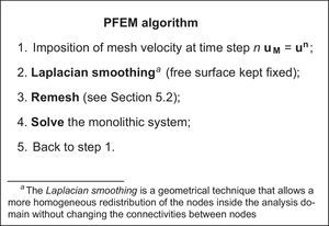

The difference between the Bingham and the proposed variable yield model can be observed in this example.

A square domain in 2D and a cubic one in 3D are pushed towards a wall.

The geometry of the models and the mesh used in both cases is shown in Fig. 2. The wall on the left side moves with constant velocity u₀ = 0.1 m/s. The material parameters are summarized in Table 4.

Fig. 2.

Pushed slope example. Geometry, mesh and boundary conditions of 2D and 3D models.

Table 4.

Pushed slope example. Material properties.

Dry density	ρ	1000 kg/m^3
Fluidified viscosity	μ	10^−6 Pa s
Smoothing coefficient	m	3000 s

For the Bingham model the yield stress is τ₀ = 1000 Pa, whereas in the variable yield model the internal friction angle is ϕ = 30.

In the sequences of the pushing process shown in Figs. 3 and 4 the different behavior of the two models is evident.

Fig. 3.

2D pushed slope. γ˙ in the initial pushing phase. Difference between the Bingham and the variable viscosity models.

Fig. 4.

2D pushed slope. γ˙ in the squeezing phase. Difference between the Bingham and the variable viscosity models.

For Bingham plastics, those points that do not exceed the constant yield threshold, behave like a rigid body, whereas in the variable yield model the yield stress of the exterior points is lower and it is exceeded also for lower pressure levels. Two different phases can be identified in the present example:

• -

  The settlement phase. It is the initial part of the example. The granular material is left free to fall and to reach its stable configuration. It goes from the beginning of the example to the moment in which the material touches the right fixed wall.

• -

  The squeezing phase. It begins when the material touches the right wall and starts to be squeezed between the two opposite walls that are getting closer.

In Fig. 3 the 2D comparison between the Bingham model and the variable yield model during the settlement phase is shown. The contour fill of the equivalent strain rate is plotted in different time instances (the blue color indicates γ˙=0).

The Bingham model shows a sliding surface where the tangential stress reaches the yield stress (1000 Pa), independently on the pressure value, whereas all the rest of the domain shows an almost rigid behavior. Conversely, in the variable yield model, if a node has a tangential stress which exceed its pressure times the friction angle tangent (p tgϕ), it shows a drop in the viscosity and it starts flowing. The main differences can be observed on the “free surface”. In the case of Bingham model any node close to the free surface has the same resistance (yield stress) than any interna node, while in the variable yield model the resistance of a superficial node is almost zero (being the pressure close to zero). The variable yield material reaches a stable configuration that respects the internal friction angle ϕ = 30°.

In Fig. 4 the behavior of the two models in the squeezing phase is compared. The sequence shows how the equivalent strain rate γ˙ is almost zero up to the creation of the failure lines and the subsequent collapse of the material. In the variable yield model, on the contrary, the “free surface” has zero pressure, which implies zero resistance and as soon as the material reaches the height of the walls, it starts falling.

The same considerations can be done in 3D, looking at the comparison between the two models in the settlement and the squeezing phase shown in Figs. 5 and 6, respectively. The Bingham model in 3D shows less resistance in the squeezing phase due to the 3-dimensional effects. It is finally interesting to observe that the material which is falling down in the case of the Bingham model conserves the velocity imposed by the wall although this is very low, whereas this does not happen in the variable yield model.

Fig. 5.

3D pushed slope. Difference between the Bingham and the variable viscosity models in the initial pushing phase.

Fig. 6.

3D pushed slope. Difference between the Bingham and the variable viscosity models in the squeezing phase.

6.2

Settlement of a vertical rockfill slope

The variable viscosity model is finally used to reproduce the settlement of a granular vertical slope with a given internal friction angle. The objective of this example is to verify the correct representation of the internal friction angle and the independence of the stable configuration from the mesh size.

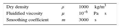
For this purpose a rectangular domain is constrained by a vertical wall in the left side and is left free on the right side as shown in Fig. 7. The material parameters are summarized in Table 5.

Fig. 7.

Settlement of a vertical slope. Geometry of the model.

Table 5.

Settlement example. Material properties.

Dry density	ρ	1000 kg/m^3
Fluidified viscosity	μ	10^−6 Pa s
Smoothing coefficient	m	3000 s

6.2.1

Variable mesh size

The internal friction angle is taken ϕ = 30°. Three different mesh sizes are taken into account for the simulation:

• •

  Mesh A is 0.1 cm. The model has 444 nodes.

• •

  Mesh B is 0.05 cm. The model has 1580 nodes.

• •

  Mesh C is 0.01 cm. The model has 35466 nodes.

They are shown in Fig. 8.

Fig. 8.

Different mesh sizes taken into account in the present example.

The evolution of the settlement is shown in Fig. 9 for the above mentioned meshes. As expected the more accurate and realistic settlement process is obtained with the finer mesh but no relevant differences appear using the coarser ones. This is respected for any internal friction angle ϕ lower or equal to 45° as will be discussed in Section 6.2.2.

Fig. 9.

Settlements for a granular slope with internal friction angle ϕ = 30° for the three different mesh sizes indicated in Fig. 8.

The same example is run in 3D using the meshes A and B of Fig. 8 leading to analogous conclusions. The internal friction angle is well represented independently from the mesh chosen. A sequence of the 3D results for a slope with internal friction angle ϕ = 30° is shown in Fig. 10.

Fig. 10.

Settlements for a 3D granular slope with internal friction angle ϕ = 30° in the case of considering mesh A and B of Fig. 8.

6.2.2

Variable internal friction angle

Different values of the internal friction angle are taken into account in order to verify the correct behavior of the structural model. Mesh B is used for the discretization.

The different mechanical behavior controlled by the values of ϕ is correctly reproduced by the variable yield model presented in this work if the internal friction angle is lower or equal to 45°, as can be observed in Fig. 11 where the stable configuration of rockfill slope of 30°, 40°, 45°and 47° is simulated. The case with ϕ = 45° represents a practical limit of the model. Beyond that limit a dependency on the mesh appears as some level of locking can be observed. The conclusion is that the model is not able to correctly simulate materials that have internal friction angles higher than 45°.

Fig. 11.

Stable results for different internal friction angles ϕ. The mesh used in the calculation is mesh B of Fig. 8.

6.3

Friction angle test

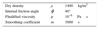
The last example simulate a test for computing the internal friction angle ϕ. A cone filled with granular material with a bottom outlet is lifted up with a velocity of 0.025 m/s. The geometry and the mesh used can be seen in Fig. 12.

Fig. 12.

Friction angle test example. Geometry and mesh used for the calculation.

The mechanical characteristics of the material used are summarized in Table 6.

Table 6.

Friction angle test example. Material properties.

Dry density	ρ	1490 kg/m^3
Internal friction angle	ϕ	40°
Fluidified viscosity	μ	10^−6 Pa s
Smoothing coefficient	m	3000 s

As expected, the final slope of the fallen material matches well with the 40° angle as shown in the last picture of Fig. 13.

Fig. 13.

Friction angle test example. Variable yield model with ϕ = 40°.

Finally in Fig. 14 the same example has been repeated in the case of a Bingham plastic with a yield threshold τ₀ = 500 Pa.

Fig. 14.

Friction angle test example. Bingham model with yield stress τ₀ = 500 Pa.

The different behaviour between the two models is evident: the material of the variable yield model “flows” down in a nearly continuous way and at the end of the simulation no material is present in the cone (the cone is 41.6° steep). Whereas the Bingham material resembles a toothpaste and at the end of the simulation part of the material remains inside the cone. The tangential stresses, in fact, are lower than the yield threshold.

7

Conclusions

In this paper a model to describe the behavior of a rockfill slope is presented. A non-Newtonian constitutive law is chosen and a regularized Bingham plastic model is developed. This choice derives from the observation that the elastic behavior in rockfill slopes is negligible and when the yield stress is reached the material starts to flow more like a fluid than to deform like a structure. Among the familiy of the non-Newtonian fluids, Bingham plastics have been chosen for their capability of supporting a certain amount of shear stress before reaching large strains.

The good behavior of the Bingham model is verified through some benchmarks, but does not seem to be adequate for the simulation of the behavior of a granular slope. For this purpose a variable yield threshold is introduced in order to mimic a Mohr Coulomb failure criterion.

The differences between the regularized Bingham and the variable yield models are discussed in some examples.

The main advantage of the constitutive law proposed is its simplicity compared with any other plastic model.

The variable yield model does not present serious limitations on the mesh sizes. Finally the variable yield model seems to be adequate to simulate materials with internal friction angles lower than 45°.

Acknowledgements

The research was supported by the Research Executive Agency through the T-MAPPP project (FP7 PEOPLE 2013 ITN-G.A.n607453). and by the European Research Council through the ERC Advanced Grant project SAFECON (AdG-267521).