Heterogeneous treatment effects in development policy evaluation: The case of the Mexican Estrategia 100×100

Abstract

A recent evaluation of the Mexican interinstitutional coordination program Estrategia 100×100, published by Coneval in 2013, did not find many satisfactory results with respect to its target population. However, in Coneval's evaluation all statistical quantities of interest were computed at the group level only, thereby overlooking individual within-group heterogeneity. In this paper we estimate the heterogeneity of these treatment effects as a function of the level of investment per capita received through the program's actions. We provide evidence that the program was in fact effective whenever it was accompanied by the required investment.

Resumen

Una evaluación reciente del programa mexicano de coordinación interinstitucional Estrategia 100×100, publicada por el Coneval en 2013, no encontró todos los resultados esperados en su población objetivo. En dicha evaluación, sin embargo, las estimaciones se llevaron a cabo sólo a nivel grupal, omitiendo analizar la posible heterogeneidad intragrupo del impacto del programa. En este artículo analizamos esta heterogeneidad como una función de la inversión per cápita erogada. Las pruebas realizadas indican que el programa obtuvo de hecho los resultados esperados cuando se acompañó de la inversión requerida.

Introduction

There is a growing body of work in the literature concerning poverty and inequality that recognizes that complex social problems, such as the reduction of regional inequalities, have multiple causes and therefore require the design and implementation of integral public policies that involve the participation of several governmental, social and private institutions which need to share information, objectives, goals and resources (Grindle, 2010; Ordaz Ocampo, 2012; Brown and Tandon, 1992; Lustig, 2001). According to Brown and Kalegoankar (2000) and Gray (1989), it is almost impossible to efficiently counteract poverty and regional inequalities by improving coverage, efficiency and sustainability of basic public delivery services without encouraging the participation of multiple actors.

It is widely recognised that integral public policies that require the coordination of several government and private institutions are key elements in both poverty and regional inequality reduction strategies. Collaboration, cooperation and coordination among different levels of government, the private sector and the civil society are aimed at overcoming obstacles such as scarcity of government resources, different government capacities and priorities, and competing demands among the different sectors involved when governments try to address regional inequalities and poverty issues.

However, this interinstitutional coordination among the different actors involved has proven to be more complex in practice than it might seem. Efforts made in the past have shown that political will by itself is not enough for coordination strategies to work. Policy designers have to develop mechanisms and rules that suit the interests of multiple diverse institutions (Grindle, 2010) through differentiated social policies according to each local and regional reality.

For this reason, the Mexican government has been implementing integral policies since the seventies in order to address poverty and regional inequalities based on interministerial coordination. For instance, the last administration implemented the umbrella program Estrategia 100×100 (E100×100) that sought to increase social and economic development in the 125 municipalities with the lowest Human Development Index (HDI) by way of 300 different actions carried out through the coordination of several government ministries and institutions. Likewise, the current federal administration has just launched the Cruzada Nacional Contra el Hambre [National Crusade Against Hunger] that has targeted the population that lives in extreme poverty with food deficiencies.

Despite advances in the role of social policy in economic development —the creation of the Consejo Nacional de Evaluación de la Política de Desarrollo Social (Coneval) [National Council for the Evaluation of Social Development Policy], for instance—, the interinstitutional coordination strategy launched by the Mexican government in recent years seems to not have had very satisfactory results in the vulnerable population they have targeted. A recent impact evaluation of E100×100 published by Coneval (2013) only found a positive impact in the reduction of the percentage of population without health insurance and the percentage of households without concrete flooring.

These results posed severe doubts concerning both the effectiveness of the E100×100 program and the cooperative efforts of governments at different levels for alleviating poverty and reducing regional inequalities. However, this evaluation was based on an Intent to Treat Model (itm) which means that the original assignment of the municipalities to E100×100 was used to carry out the analysis instead of the effective reception of the treatment, mainly due to the difficulty of measuring the actual interinstitutional coordination. Hence, as Outhwaite and Turner (2008) suggested, under the itm, finding a non-statistically significant difference between the treatment and the control group cannot be interpreted as if receiving or not the treatment produces equivalent results. It could have been that the treatment spilled out to some of the control units—as argued by Coneval in their evaluation. In Coneval's evaluation, all statistical quantities of interest were computed only at the group level, overlooking individual within-group level variations or heterogeneity which, according to the data provided by Secretaría de Desarrollo Social (Sedesol) [Ministry of Social Development], exists in terms of the investment per capita received through the program's specific actions across treated municipalities. It is important to mention that the investment data was available only for municipalities that were part of E100×100, so the possibility of using investment as the treatment variable was not possible.

The hypothesis of this paper is that E100×100's intervention is best captured not only by the treatment status of the municipalities, but also through the different levels of investment per capita among the treated municipalities. Therefore, the results varied widely, depending upon whether E100×100's intervention included the financial resources dearly needed in the treated municipalities, diluting any treatment effect estimated using only the assignment to the program as treatment variable. In this paper, we put to empirical test this hypothesis assessing the heterogeneity in previously estimated treatment effects as a function of the level of investment per capita. Unfortunately, whether the observed variability in investment per capita speaks of the degree of coordination actually achieved by the officials involved is a whole different matter which we cannot assert with the available data.

There are, however, two reasons why we see the investment per capita as part of E100×100's intervention, irrespective of the terms in which this might have happened. Firstly, all the investment we have taken into account in our analysis ran through the E100×100. That is, we have only used the investment for which the coordination effort can be credited. Secondly, even though the investment was prominently federal (87%), this does not mean it required no involvement of the E100×100. All federal social programs that worked within the framework of E100×100, and through which the investments were made, had as part of their target population all of the 125 municipalities on which the E100×100 was focused. This left in sight no other obvious culprit for the observed differences in investment per capita but the inner workings of E100×100, especially among paired municipalities.

A word of caution is warranted though. Admittedly, exactly how correlated is this investment data with an actual measure of E100×100's effectiveness is a pending task in the literature, and our results should be read accordingly. Ultimately, the readers can make their own conclusions based on the heterogeneity analysis presented here.

This analysis was performed following the practical approach proposed by Xie, Brand, and Jann (2012)¹ based on observational data using Propensity Score Matching (PSM). Hence, the empirical strategy consisted of firstly, the replication of the Propensity Score (PS) estimates carried out in Coneval's evaluation using the same set of observed pre-treatment covariates for each municipality with the same sample consisting of the 2 456 municipalities throughout the country. Secondly, a multiple matching based on the PS estimated was used to transform the data into treatment-control comparisons replicating the estimation of Average Treatment Effects (ATT). Thirdly, the observed difference in pairs between treated municipalities and the group mean of the multiple matched controls (the matched difference for the ATT) was used to estimate the heterogeneous treatment effects as a function of the relevant investment per capita data by fitting a linear parametric model to evaluate trends across the municipalities.

The paper is organised as follows: Section 2 succinctly describes the coordination efforts implemented by the Mexican government up till the E100×100 umbrella program was launched. Section 3 reviews the impact evaluation published by Coneval. Section 4 describes the data and the methodology employed to assess the heterogeneity of the treatment effects of E100×100 as a function of the different levels of investment per capita received through the program's specific actions. Section 5 presents the key results and section 6 discusses and concludes these findings.

Previous coordination efforts up to theE100×100 program

Since the seventies, the Mexican government has been trying to alleviate complex social problems with the implementation and design of integral strategies based on interinstitutional coordination. In this sense, the idea of the necessity of integral public policies in Mexico is not new. However, as Ordaz Ocampo (2102) argues, the existence of power asymmetries has led to results that were less favourable than expected.

Probably the first attempt of this kind of programs occurred in 1973 with the implementation of the Programa de Inversión de Desarrollo Rural (PIDER) [Public Investment Program for Rural Development]. Its main objective was the promotion of integral rural development through the participation of the three levels of government. However, the integral approach and its transversal nature surpassed the public administration's capacity and ultimately generated actions that were not a product of this desired coordination among different government institutions (Herrera, 2007).

By 1977, the Coordinación General del Plan Nacional de Zonas Deprimidas y Grupos Marginados (coplamar) [General Coordination for the National Plan of Depressed Zones and Marginal Groups], was created with the explicit objective of reducing levels of exclusion of farmers, migrants and indigenous people, among others. According to Ordaz Ocampo (2012), both pider and coplamar were undermined by the lack of public officials skilled in decisionmaking and with broad authority to determine the appropriate actions for local circumstances.

In 1994, the Congress declared as Zonas de Atención Prioritaria (zap) [Priority Attention Areas], the most vulnerable geographic areas on which development policies should focus their attention. This was part of the efforts for improving the design of public policies aimed at enhancing the integral development of the municipalities with the highest levels of social exclusion and poverty.

In 2000, the new administration launched the Estrategia Microregiones program [Micro-regions Strategy]. This program was meant to improve the wellbeing of the most disadvantaged part of the population who had been excluded from the provision of basic infrastructure and services due to their geographical dispersion and isolation, the low capacities of local governments. This involved the participation of multiple government officials, the private sector and the community, but in practice, the support came almost entirely from the highest Federal level mainly due to the change of the political party in power and the coexistence of different ideological views (itesm, 2007).

With the same spirit of tackling regional inequalities and poverty, in 2006 the Mexican government launched yet another interinstitutional coordination program called Estrategia 100×100 (E100×100), having as its main objective the increase of social and economic development in the 125 municipalities with the lowest HDI and highest levels of social exclusion.

The E100×100 umbrella program had two specific objectives: 1) To increase the income of the population who lived in these most disadvantageous 125 municipalities through actions oriented to increase productivity and employment opportunities and 2) To increase their quality of life through improvements in both the access and quality to health and education services as well as the housing and infrastructure conditions.

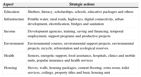
Through over 300 specific interventions carried out by several Government Ministries, the program was aimed at improving the wellbeing of the most vulnerable part of the population focusing on education, health, income, housing, infrastructure and environment. These interventions were grouped in what was then called “strategic actions” as shown in Table 1.

Table 1.

Aspects and actions of the E100×100 program.

Aspect	Strategic actions
Education	Shelters, literacy, scholarships, schools, educative packages and others
Infrastructure	Potable water, rural roads, highways, digital connectivity, urban development, electrification, bridges and sanitation
Income	Development agencies, training, saving and financing, temporal employment, support programs and productive projects
Environment	Environmental courses, environmental support projects, environmental projects, recycle, reforestation and ecological reserves
Health	Seniors, energetic support, food assistance, hospitals, clinics and mobile units, popular insurance and health services
Housing	Stoves, walls, housing packages, cement flooring, extra room, toilet services, ceilings, property titles and basic housing unit

Source: Estrategia 100×100. Available at: <http://www.estrategia100×100.gob.mx>.

The E100×100 program was a coordination scheme meant to link and complement the different actions carried out by several government branches through approximately 70 different development programs, all of them aimed at confronting regional inequalities and reducing poverty through the coordination of 14 Ministries and agencies of the Federal Government, 7 State Governments and 125 Municipality Governments over the 6 different aspects that were meant to improve the wellbeing of the population. Each of these 6 aspects of the E100×100 had an inter-ministry thematic working group within the Comisión Intersecretarial de Desarrollo Social (CIDS) [Interministry Commission for Social Development], which was in charge of establishing the conceptual and operational basis for the coordination both at the central and state level. The Technical Secretary presiding over these thematic working groups was the Secretaría de Desarrollo Social (Sedesol) [Minister of Social Development] with the goal of ensuring coordination and communication among them. Coordinating each thematic group was the responsibility of the head of the respective Ministry who was responsible for monitoring all investment plans and defining both the specific performance indicators and the targets to be achieved.

In summation, the E100×100 was not a program of the Federal Government in the sense of having its own budget, but it was a scheme for the coordination of joint actions by different federal programs to promote the economic and social development. The E100×100 did not “plan” as much as it “manage”.

According to data provided by Sedesol for the period of 2007-2011, approximately 39 544 million pesos (some 2 950 million usd of the time) were spent as part of the actions carried out by E100×100 from which 87% represented federal investment, 10% was state investment and only 3% represented municipal investment. From the grand total, the Sedesol contributed with the largest investment representing 45.6% of the total, followed by the Comisión Nacional para el Desarrollo de los Pueblos Indigenas (cdi) [National Commission for the Development of Indigenous Populations] with 17.3%, while the Ministries of Education and Health only contributed 3.4% and 2.5% respectively.

Previous impact evaluation of E100×100

In order to identify the effects of E100×100 regarding one of its objectives—the improvement of living conditions—, in 2012 Coneval carried out an intention-to-treat evaluation of the program by making use of public information of the 2,456 municipalities in the country, mainly from the Censo de Población y Vivienda [Population and Housing Census] from 2000 and 2010 and the Conteo de Población y Vivienda [Population and Housing Count] from 2005, drawing on this last one for baseline covariates.²

The causal treatment effects of the E100×100 program —under the assumption of treatment homogeneity— were estimated for several performance indicators including components of the hdi³, the Índice de Desarrollo Social (irs)⁴ [Social Gap Index], and the Índice de Marginación (im)⁵ [Marginalization Index]. The identification strategy to estimate the treatment effects was selection on observable factors, making use of PSM and Regression Discontinuity Design. Additionally, psm was combined with Differences in Differences in order to control for unobservable characteristics that remained constant over time but that could have influenced selection into treatment and potential outcomes.⁶

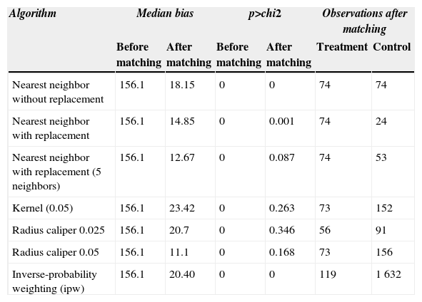
Table 2 reproduces the main diagnostics of the different PSM algorithms employed in Coneval's evaluation.⁷

Table 2.

Diagnostic tests before and after matching.

Algorithm	Median bias		p>chi2		Observations after matching
	Before matching	After matching	Before matching	After matching	Treatment	Control
Nearest neighbor without replacement	156.1	18.15	0	0	74	74
Nearest neighbor with replacement	156.1	14.85	0	0.001	74	24
Nearest neighbor with replacement (5 neighbors)	156.1	12.67	0	0.087	74	53
Kernel (0.05)	156.1	23.42	0	0.263	73	152
Radius caliper 0.025	156.1	20.7	0	0.346	56	91
Radius caliper 0.05	156.1	11.1	0	0.168	73	156
Inverse-probability weighting (ipw)	156.1	20.40	0	0	119	1 632

Note: p-values correspond to the likelihood-ratio test of the joint insignificance of all the regressors before and after matching.

Source: Coneval (2013) and own calculations.

Several points are worth mention. It is important to notice that in Coneval's evaluation no good matching was possible for the 125 treated municipalities. With the best matching algorithm, radius caliper of 0.05 according to Coneval's evaluation, 52 treatment municipalities were discarded, that is, the treatment effect for these municipalities could not have been estimated because it was not possible to find them a good match, i.e., the closest control municipality for each of them had a propensity score “farther away” than 0.05. Note that even though the inverse-probability weighting estimator (ipw) made use of most of the data, Table 2 shows that the p-values of the likelihood-ratio test of the joint insignificance of all the regressors, before and after matching, were both zero, and that it exhibited the second larger value for the median of the standardized bias.

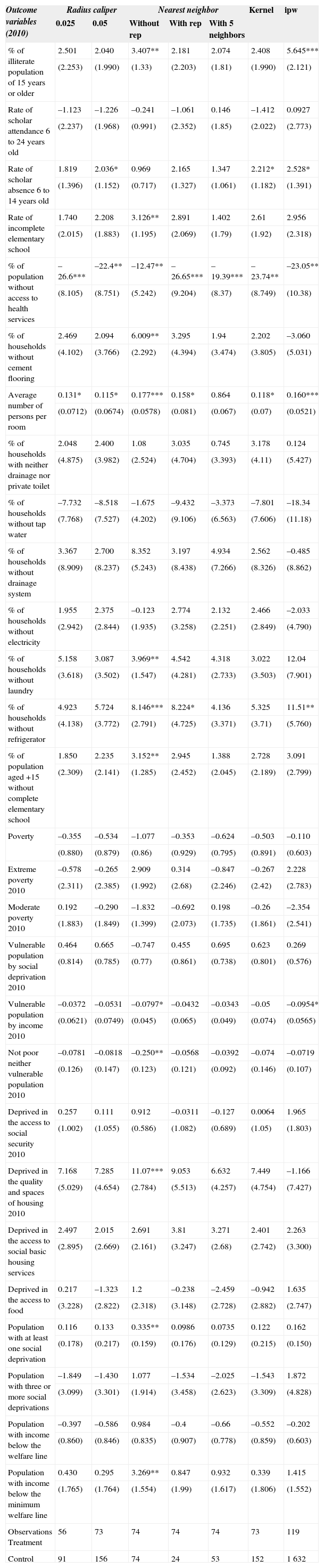
For completeness, Tables 3 and 4 reproduce, in levels and differences respectively and for every PSM algorithm, the estimated effect of the E100×100 program on the outcome variables analyzed in Coneval's evaluation.

Table 3.

ATT in levels of 2010.

Outcome variables (2010)	Radius caliper		Nearest neighbor			Kernel	ipw
	0.025	0.05	Without rep	With rep	With 5 neighbors
% of illiterate population of 15 years or older	2.501	2.040	3.407**	2.181	2.074	2.408	5.645***
	(2.253)	(1.990)	(1.33)	(2.203)	(1.81)	(1.990)	(2.121)
Rate of scholar attendance 6 to 24 years old	–1.123	–1.226	–0.241	–1.061	0.146	–1.412	0.0927
	(2.237)	(1.968)	(0.991)	(2.352)	(1.85)	(2.022)	(2.773)
Rate of scholar absence 6 to 14 years old	1.819	2.036*	0.969	2.165	1.347	2.212*	2.528*
	(1.396)	(1.152)	(0.717)	(1.327)	(1.061)	(1.182)	(1.391)
Rate of incomplete elementary school	1.740	2.208	3.126**	2.891	1.402	2.61	2.956
	(2.015)	(1.883)	(1.195)	(2.069)	(1.79)	(1.92)	(2.318)
% of population without access to health services	–26.6***	–22.4**	–12.47**	–26.65***	–19.39***	–23.74**	–23.05**
	(8.105)	(8.751)	(5.242)	(9.204)	(8.37)	(8.749)	(10.38)
% of households without cement flooring	2.469	2.094	6.009**	3.295	1.94	2.202	–3.060
	(4.102)	(3.766)	(2.292)	(4.394)	(3.474)	(3.805)	(5.031)
Average number of persons per room	0.131*	0.115*	0.177***	0.158*	0.864	0.118*	0.160***
	(0.0712)	(0.0674)	(0.0578)	(0.081)	(0.067)	(0.07)	(0.0521)
% of households with neither drainage nor private toilet	2.048	2.400	1.08	3.035	0.745	3.178	0.124
	(4.875)	(3.982)	(2.524)	(4.704)	(3.393)	(4.11)	(5.427)
% of households without tap water	–7.732	–8.518	–1.675	–9.432	–3.373	–7.801	–18.34
	(7.768)	(7.527)	(4.202)	(9.106)	(6.563)	(7.606)	(11.18)
% of households without drainage system	3.367	2.700	8.352	3.197	4.934	2.562	–0.485
	(8.909)	(8.237)	(5.243)	(8.438)	(7.266)	(8.326)	(8.862)
% of households without electricity	1.955	2.375	–0.123	2.774	2.132	2.466	–2.033
	(2.942)	(2.844)	(1.935)	(3.258)	(2.251)	(2.849)	(4.790)
% of households without laundry	5.158	3.087	3.969**	4.542	4.318	3.022	12.04
	(3.618)	(3.502)	(1.547)	(4.281)	(2.733)	(3.503)	(7.901)
% of households without refrigerator	4.923	5.724	8.146***	8.224*	4.136	5.325	11.51**
	(4.138)	(3.772)	(2.791)	(4.725)	(3.371)	(3.71)	(5.760)
% of population aged +15 without complete elementary school	1.850	2.235	3.152**	2.945	1.388	2.728	3.091
	(2.309)	(2.141)	(1.285)	(2.452)	(2.045)	(2.189)	(2.799)
Poverty	–0.355	–0.534	–1.077	–0.353	–0.624	–0.503	–0.110
	(0.880)	(0.879)	(0.86)	(0.929)	(0.795)	(0.891)	(0.603)
Extreme poverty 2010	–0.578	–0.265	2.909	0.314	–0.847	–0.267	2.228
	(2.311)	(2.385)	(1.992)	(2.68)	(2.246)	(2.42)	(2.783)
Moderate poverty 2010	0.192	–0.290	–1.832	–0.692	0.198	–0.26	–2.354
	(1.883)	(1.849)	(1.399)	(2.073)	(1.735)	(1.861)	(2.541)
Vulnerable population by social deprivation 2010	0.464	0.665	–0.747	0.455	0.695	0.623	0.269
	(0.814)	(0.785)	(0.77)	(0.861)	(0.738)	(0.801)	(0.576)
Vulnerable population by income 2010	–0.0372	–0.0531	–0.0797*	–0.0432	–0.0343	–0.05	–0.0954*
	(0.0621)	(0.0749)	(0.045)	(0.065)	(0.049)	(0.074)	(0.0565)
Not poor neither vulnerable population 2010	–0.0781	–0.0818	–0.250**	–0.0568	–0.0392	–0.074	–0.0719
	(0.126)	(0.147)	(0.123)	(0.121)	(0.092)	(0.146)	(0.107)
Deprived in the access to social security 2010	0.257	0.111	0.912	–0.0311	–0.127	0.0064	1.965
	(1.002)	(1.055)	(0.586)	(1.082)	(0.689)	(1.05)	(1.803)
Deprived in the quality and spaces of housing 2010	7.168	7.285	11.07***	9.053	6.632	7.449	–1.166
	(5.029)	(4.654)	(2.784)	(5.513)	(4.257)	(4.754)	(7.427)
Deprived in the access to social basic housing services	2.497	2.015	2.691	3.81	3.271	2.401	2.263
	(2.895)	(2.669)	(2.161)	(3.247)	(2.68)	(2.742)	(3.300)
Deprived in the access to food	0.217	–1.323	1.2	–0.238	–2.459	–0.942	1.635
	(3.228)	(2.822)	(2.318)	(3.148)	(2.728)	(2.882)	(2.747)
Population with at least one social deprivation	0.116	0.133	0.335**	0.0986	0.0735	0.122	0.162
	(0.178)	(0.217)	(0.159)	(0.176)	(0.129)	(0.215)	(0.150)
Population with three or more social deprivations	–1.849	–1.430	1.077	–1.534	–2.025	–1.543	1.872
	(3.099)	(3.301)	(1.914)	(3.458)	(2.623)	(3.309)	(4.828)
Population with income below the welfare line	–0.397	–0.586	0.984	–0.4	–0.66	–0.552	–0.202
	(0.860)	(0.846)	(0.835)	(0.907)	(0.778)	(0.859)	(0.603)
Population with income below the minimum welfare line	0.430	0.295	3.269**	0.847	0.932	0.339	1.415
	(1.765)	(1.764)	(1.554)	(1.99)	(1.617)	(1.806)	(1.552)
Observations Treatment	56	73	74	74	74	73	119
Control	91	156	74	24	53	152	1 632

Source: Coneval (2013) and own calculations.

Table 4.

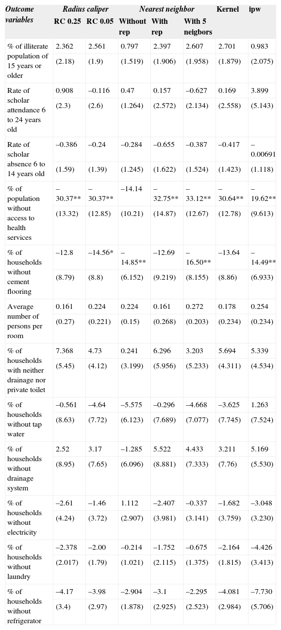
att in Differences in Differences.

Outcome variables	Radius caliper		Nearest neighbor			Kernel	ipw
	RC 0.25	RC 0.05	Without rep	With rep	With 5 neigbors
% of illiterate population of 15 years or older	2.362	2.561	0.797	2.397	2.607	2.701	0.983
	(2.18)	(1.9)	(1.519)	(1.906)	(1.958)	(1.879)	(2.075)
Rate of scholar attendance 6 to 24 years old	0.908	–0.116	0.47	0.157	–0.627	0.169	3.899
	(2.3)	(2.6)	(1.264)	(2.572)	(2.134)	(2.558)	(5.143)
Rate of scholar absence 6 to 14 years old	–0.386	–0.24	–0.284	–0.655	–0.387	–0.417	–0.00691
	(1.59)	(1.39)	(1.245)	(1.622)	(1.524)	(1.423)	(1.118)
% of population without access to health services	–30.37**	–30.37**	–14.14	–32.75**	–33.12**	–30.64**	–19.62**
	(13.32)	(12.85)	(10.21)	(14.87)	(12.67)	(12.78)	(9.613)
% of households without cement flooring	–12.8	–14.56*	–14.85**	–12.69	–16.50**	–13.64	–14.49**
	(8.79)	(8.8)	(6.152)	(9.219)	(8.155)	(8.86)	(6.933)
Average number of persons per room	0.161	0.224	0.224	0.161	0.272	0.178	0.254
	(0.27)	(0.221)	(0.15)	(0.268)	(0.203)	(0.234)	(0.234)
% of households with neither drainage nor private toilet	7.368	4.73	0.241	6.296	3.203	5.694	5.339
	(5.45)	(4.12)	(3.199)	(5.956)	(5.233)	(4.311)	(4.534)
% of households without tap water	–0.561	–4.64	–5.575	–0.296	–4.668	–3.625	1.263
	(8.63)	(7.72)	(6.123)	(7.689)	(7.077)	(7.745)	(7.524)
% of households without drainage system	2.52	3.17	–1.285	5.522	4.433	3.211	5.169
	(8.95)	(7.65)	(6.096)	(8.881)	(7.333)	(7.76)	(5.530)
% of households without electricity	–2.61	–1.46	1.112	–2.407	–0.337	–1.682	–3.048
	(4.24)	(3.72)	(2.907)	(3.981)	(3.141)	(3.759)	(3.230)
% of households without laundry	–2.378	–2.00	–0.214	–1.752	–0.675	–2.164	–4.426
	(2.017)	(1.79)	(1.021)	(2.115)	(1.375)	(1.815)	(3.413)
% of households without refrigerator	–4.17	–3.98	–2.904	–3.1	–2.295	–4.081	–7.730
	(3.4)	(2.97)	(1.878)	(2.925)	(2.523)	(2.984)	(5.706)

Note: The differences taken correspond to the years 2010-2005-(2005-2000). Standard errors in parentheses: *** p < 0.01, ** p < 0.05, * p < 0.1. Source: Coneval (2013) and own calculations.

From the 29 outcome variables analyzed in this evaluation, according to the matching algorithm favored by Coneval, statistically significant results were found only in the reduction of the percentage of population without access to health services and in the reduction of the percentage of households without cement flooring. However, this last result was not robust for all the different samples and specifications employed. The improvement in conditions regarding the lack of access to health services was 30.4%. A figure that represents a reduction in the performance indicator of 47.3% with respect to the control group (Coneval, 2013).

However, it is important to recall that this evaluation was based on the ITM so if the results did not show significant differences between the treatment and the control municipalities in the relevant outcome variables over which the impact was measured, this should not be interpreted as if the E100×100 program did not have the desired impact on their beneficiaries. As mentioned before, under the itm, it was not possible to determine whether some of the treated municipalities ended up being untreated or if some of the control municipalities actually received the treatment due to spillover effects. In other words, all we know is that municipalities in the sample ended up being treated alike —i.e. missing or receiving the treatment— and therefore responding alike (Outhwaite and Turner, 2008) on the average.

Accordingly, the conclusions of the evaluation performed by Coneval state that it could have been the case that the actions of the different federal social programs coordinated by the E100×100 umbrella program did not focus only on the 125 most vulnerable municipalities, but covered all municipalities with high irs, the control group among them. In summary, there was no evidence to state that there was a singular prioritization of these 125 municipalities in contrast with other poor municipalities of the country. It merits attention the fact that the only outcomes in which the evaluation found the expected results were associated to two highly centralized subprograms: Seguro Popular [Popular Insurance] and Piso Firme [Concrete Flooring], presumably two subprograms that didn’t require much coordination.

In Coneval's evaluation, all statistical quantities of interest were computed only at the group level —under the assumption of treatment homogeneity—, overlooking within-group heterogeneity which existed in terms of the investment per capita received through the program's specific actions across different municipalities. Heterogeneous treatment effects are seldom studied empirically in the evaluation of development programs, regardless of their important implications for social policy. On the one hand, if policy makers understand patterns of treatment effect heterogeneity, they can more effectively concentrate their efforts where they are more sorely needed. On the other hand, the study of treatment effect heterogeneity can also yield important insights about how scarce social resources are distributed in an unequal society (Xie, Brand, and Jann, 2012; Manski, 2007).

In this paper we followed Xie, Brand, and Jann (2012) in their approach to studying treatment effect heterogeneity that builds on the same framework for estimating the causal effects. That is, under the ignorability or selection on observables assumption. The ignorability assumption allows the researcher to explore empirical patterns of treatment effect heterogeneity as a function of other variables such as the propensity score itself and in our case of investment per capita disaggregated by specific action of the program, which in turn it was taken as differences in the actual treatment received by the municipalities. This strategy was followed in view of the lack of any additional information regarding the actual coordination achieved by program.

Data

For the replication of the results estimated in Coneval's evaluation, we used the same data on socioeconomic conditions, social gaps, levels of marginalization and poverty from the 2 456 municipalities of the country contained in the Censo de Población y Vivienda of 2000 and 2010, the Conteo de Población y Vivienda of 2005, the municipal hdi, the irs and the im.

The 125 treated municipalities of the E100×100 program comprised the 100 municipalities with the lowest HDI in the year of 2000 and the 25 municipalities, identified by Coneval, both with a high level of social exclusion and more than 60 per cent of their population living under food poverty. Whereas the pool of control municipalities consisted of the rest of the municipalities of the country. That is, 2 331 municipalities comprised the pool from which the comparison group were matched.

Additionally, for the estimation of the heterogeneity in treatment effects, this paper used information provided by the Sedesol regarding the level of investment by Strategic Actions for each of the 125 treated municipalities from 2007 to 2011. It is important to recall that this investment data was not available for the 2 331 non-treated municipalities of the sample. Note also that the investment data we used in our estimates was produced as a byproduct of the E100×100 and no similar data exists for any other municipality apart from the 125 that comprised its target population. By no means this is to say that none of the other municipalities excluded from the E100×100 received any investment, or that they were not part of the target population of other, or even the same, social programs. The social programs themselves did not constitute the E100×100 for it was a coordination scheme.

This is why it was impossible to use the investment variable as the treatment. Instead, the investment per capita by Strategic Action in each of the 125 treated municipalities was taken as differences in the intervention that actually took place.

According to the yearly investment data provided by Sedesol, the global investment per capita by Aspect at the municipal level has been unequal among treated municipalities for the period 2007-2011. For instance, the municipality of Mezquital in the northern State of Durango received 8.7 more resources per capita than San Simón Zahuatlán in the south state of Oaxaca for the period of 2007-2011. On average the former municipality received 3.1 more resources than the rest of the municipalities that were part of E100×100. In this paper we exploited this variability to get a feeling of the effect that different versions of E100×100's intervention had on the outcome variables employed in Coneval's analysis.

Regarding the quality of the investment data, it is important to keep in mind that we used it as it was provided by Sedesol: with minimum disaggregation of the specific institution financially responsible for the spending or the specific kind of service delivered. These were aggregate figures and should not be interpreted as an exhaustive account of the money spent in the municipalities that comprised the E100×100 target population in that period. However, it was not our intention to use the investment data to estimate the true cost of observing a desired effect on the most vulnerable territories in the country. Rather, in this paper we used the variability in the data as an indicator of the particular intervention that took place in each of the 125 municipalities. As long as whatever quality issues in the data apply to all municipalities, and we had no reason to believe this was not the case, we were on safe ground assuming the data fit our purposes.

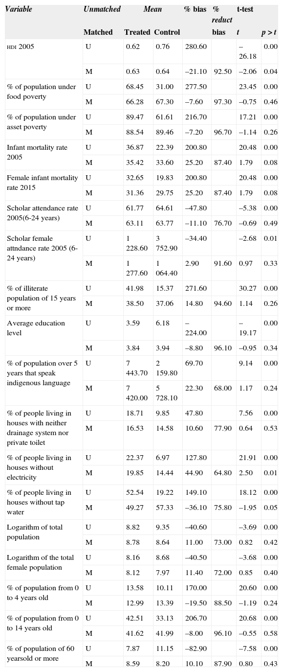
Homogeneous treatment effects estimates, a replication of the propensity score and matching estimates

As mentioned before, as a first step to estimate the heterogeneity in treatment effects, we had replicated the matching procedure championed in Coneval's evaluation: radius matching with a maximum distance of 0.05 for controls. Table 5 shows mean-comparison tests of several variables as balance diagnostics for comparing the distribution of baseline covariates between treatment groups.

Table 5.

Mean-comparison tests between treatment groups (Radius caliper 0.05).

Variable	Unmatched	Mean		% bias	% reduct	t-test
	Matched	Treated	Control		bias	t	p > t
hdi 2005	U	0.62	0.76	280.60		–26.18	0.00
	M	0.63	0.64	–21.10	92.50	–2.06	0.04
% of population under food poverty	U	68.45	31.00	277.50		23.45	0.00
	M	66.28	67.30	–7.60	97.30	–0.75	0.46
% of population under asset poverty	U	89.47	61.61	216.70		17.21	0.00
	M	88.54	89.46	–7.20	96.70	–1.14	0.26
Infant mortality rate 2005	U	36.87	22.39	200.80		20.48	0.00
	M	35.42	33.60	25.20	87.40	1.79	0.08
Female infant mortality rate 2015	U	32.65	19.83	200.80		20.48	0.00
	M	31.36	29.75	25.20	87.40	1.79	0.08
Scholar attendance rate 2005(6-24 years)	U	61.77	64.61	–47.80		–5.38	0.00
	M	63.11	63.77	–11.10	76.70	–0.69	0.49
Scholar female attndance rate 2005 (6-24 years)	U	1 228.60	3 752.90	–34.40		–2.68	0.01
	M	1 277.60	1 064.40	2.90	91.60	0.97	0.33
% of illiterate population of 15 years or more	U	41.98	15.37	271.60		30.27	0.00
	M	38.50	37.06	14.80	94.60	1.14	0.26
Average education level	U	3.59	6.18	–224.00		–19.17	0.00
	M	3.84	3.94	–8.80	96.10	–0.95	0.34
% of population over 5 years that speak indigenous language	U	7 443.70	2 159.80	69.70		9.14	0.00
	M	7 420.00	5 728.10	22.30	68.00	1.17	0.24
% of people living in houses with neither drainage system nor private toilet	U	18.71	9.85	47.80		7.56	0.00
	M	16.53	14.58	10.60	77.90	0.64	0.53
% of people living in houses without electricity	U	22.37	6.97	127.80		21.91	0.00
	M	19.85	14.44	44.90	64.80	2.50	0.01
% of people living in houses without tap water	U	52.54	19.22	149.10		18.12	0.00
	M	49.27	57.33	–36.10	75.80	–1.95	0.05
Logarithm of total population	U	8.82	9.35	–40.60		–3.69	0.00
	M	8.78	8.64	11.00	73.00	0.82	0.42
Logarithm of the total female population	U	8.16	8.68	–40.50		–3.68	0.00
	M	8.12	7.97	11.40	72.00	0.85	0.40
% of population from 0 to 4 years old	U	13.58	10.11	170.00		20.60	0.00
	M	12.99	13.39	–19.50	88.50	–1.19	0.24
% of population from 0 to 14 years old	U	42.51	33.13	206.70		20.68	0.00
	M	41.62	41.99	–8.00	96.10	–0.55	0.58
% of population of 60 yearsold or more	U	7.87	11.15	–82.90		–7.58	0.00
	M	8.59	8.20	10.10	87.90	0.80	0.43

Source: Own elaboration.

It's important to note that all variables exhibited major reductions in the standardized bias. Also in none of them was possible to reject the hypothesis of the equality of the means between treated and control after matching with a p-value smaller than 0.01, and only in two cases with p-value smaller than 0.05. Moreover, there was added value in using exactly the same matching as the one in Coneval's evaluation, for it allowed us to reexamine Coneval's conclusions in its own terms, providing evidence of heterogeneous treatment effects of the E100×100 program, something that remained a conjecture in the original evaluation.

Remember that these matching results were based on the ITM which means that the original assignment of the municipalities to E100×100 was used to carry out the analysis instead of the effective reception of the treatment, that in this case would’ve correspond to the actual degree of coordination achieved by the different institutions part of the E100×100.

Also of importance is the fact that the treated municipalities that were unmatched using the radius matching algorithm of 0.05 are the ones which have the worst conditions among all the treated ones. This explains why it was not possible to find a good match for them since they were the most disadvantaged municipalities among the rest that were part of the E100×100 program. Hence, let's keep in mind that what follows, as Coneval's conclusions, is based only on the 73 treated municipalities for which a good match was found.

At this point we used the level of investment per capita received through the program's specific actions as a sign of the mixed nature of E100×100's intervention to uncover any underlying systematic heterogeneity in the effects of the E100×100 program.

As the annual investment data show, municipalities in the E100×100 program differed greatly in the particular “treatment” they received as the amount of investment per capita varies across municipalities. Provided the amount of investment per capita reflects differences in the intervention orchestrated by E100×100, it was to be expected that municipalities whose treatment included the required financial resources would observe the expected effects.

Heterogeneous treatment effects estimates

The hypothesis of our paper is that, provided the different levels of investment per capita by specific action among the 125 treated municipalities reflects actual differences in E100×100's intervention, municipalities differ not only in their treatment status but also in the particular treatment they received. Thus, a systematic heterogeneity in the treatment effects estimated by Coneval was expected to be shaped depending on whether the intervention was accompanied by the resources dearly needed in the treated municipalities.

In order to estimate the heterogeneous treatment effects as a function of the investment per capita, for every outcome variable, the observed difference in a pair between a treated municipality and the group mean of the multiple matched controls municipalities was estimated. That is, following Xie, Brand, and Jann (2012), the data was transformed so that the differences in pairs between matched treated and control municipalities constituted the “observed” data subject to further modeling. In other words, the “raw” data for the next step were observational differences of matched comparisons for each outcome variable in this third step.

These differences were used to run a parametric model (Ordinary Least Squares) to assess the statistical significance of a linear trend of the treatment effect heterogeneity as a function of the associated actions’ investment per capita level.⁸ Of course, more flexible modeling devices could be used to fit the data such as locally weighted regression. We also followed this approach, which we don’t show here for reasons of space, and the results suggest the linear trend as a good approximation.

Models with a significant linear trend were analyzed to answer whether or not, when E100×100's intervention included a minimum of financial resources, the impact estimated for those particular municipalities were the desired ones.

Whenever a statistical significance linear trend was found in the analysis of every action associated to the outcome variable subject of study, the differences between the treated municipalities and the group mean of the multiple matched controls were plotted along the level of investment per capita —in the x-axis. This allowed us to analyze the relation between the observed differences of matched comparisons —for each of the 29 outcome variables— and the investment per capita by specific action in the treated municipalities (the heterogeneous treatment effects).

Additionally as Xie, Brand, and Jann (2012) suggest, the treatment effects may vary systematically by the propensity score for treatment due to heterogeneity population composition. Hence, the observed matched differences were also plotted against the propensity score in order to study the heterogeneity in treatment effects as a function of the probability of receiving treatment. The propensity score itself was an index of social exclusion in this case. This was done in order to find evidence on which treated municipalities benefited more from E100×100 and therefore provided evidence that could be used by policy makers in order to assign resources more effectively.

Results

For reasons of space, and to avoid flooding the reader with numbers, this section presents only part of the results of the regression analysis of the matched differences against investment per capita disaggregated by specific actions. Only those actions that were expected to have a direct impact on the outcome variable in question were reported in this section. We’ve also omitted the results for the outcome variables for which no statistically significant —robust errors were taken into account whenever they were bigger than the usual errors— relations were found.⁹

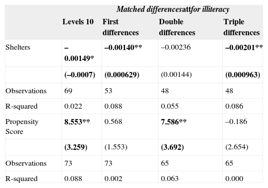
Table 6 shows the main results of the analysis of treatment heterogeneity for the percentage of illiterate population of 15 years and older in the municipality.

Table 6.

Heterogeneity analysis for illiteracy.

	Matched differencesattfor illiteracy
	Levels 10	First differences	Double differences	Triple differences
Shelters	–0.00149*	–0.00140**	–0.00236	–0.00201**
	(–0.0007)	(0.000629)	(0.00144)	(0.000963)
Observations	69	53	48	48
R-squared	0.022	0.088	0.055	0.086
Propensity Score	8.553**	0.568	7.586**	–0.186
	(3.259)	(1.553)	(3.692)	(2.654)
Observations	73	73	65	65
R-squared	0.088	0.002	0.063	0.000

Note: The ols regressions were run with robust standard errors and standard errors being the larger errors the ones who are reported in parentheses: *** p < 0.01, ** p < 0.05, * p < 0.1. First difference: illiteracy 2010- illiteracy 2005; Double differences: illiteracy 2010-(illiteracy 2005-illiteracy 2000); Triple differences: illiteracy 2010-illiteracy 2005-(illiteracy 2005-2000).

Source: Own elaboration.

From these results it can be seen that the coefficient of investment per capita for the action of Shelters¹⁰ is statistically significant and negative for three of the estimated differences: the simple difference taken in 2010 on the matched municipalities; first differences, that is the difference in difference 2010-2005 and the difference in difference that discounts the difference in the observed trend 2005-2000. All of this suggests that there was a positive impact on the reduction of the expected illiteracy as the level of investment per capita for Shelters actions increased.

This is illustrated in Figure 1 where the difference between a treated municipality and the group mean of the multiple matched controls is plotted against the investment per capita in Shelters. The figure also depicts the lowess or fully nonparametric estimation for the same variables and it seems that for this specific case linearity is a reasonable functional form.

Figure 1.

Heterogeneity analysis for Illiteracy: Shelters.

These results, we argue, were informative enough to assert that in those treated municipalities where the intervention was accompanied by investment in Shelters, the impact on the reduction of illiteracy was larger than in those municipalities in which the intervention didn’t secure a minimum of financial resources. It is in this heterogeneity that the estimated impact in Coneval's evaluation got lost.

Table 6 also presents the results of the analysis where the heterogeneous treatment effects of the program were estimated as a function of the PS to treatment. The coefficient of the PS was statistically significant and positive for the simple difference in levels and the double difference 2010-(2005-2000).

Thus, as it can be seen in figure 2, the expected impact of E100×100 on the reduction of illiteracy was largest for the municipalities that had a lower PS—and therefore less likely to be assigned into the program— and attenuates as poorer municipalities —the ones with greater propensity scores and therefore more vulnerable— were considered.

Figure 2.

Heterogeneity analysis for Illiteracy: ps.

This implies that the municipalities that have a greater PS —the ones who are most likely to be part of the program— are the ones who are benefiting less from it. Together, these results provided compelling quantitative evidence that the E100×100 program has proven most helpful in less vulnerable territories, leaving behind those in greater need.

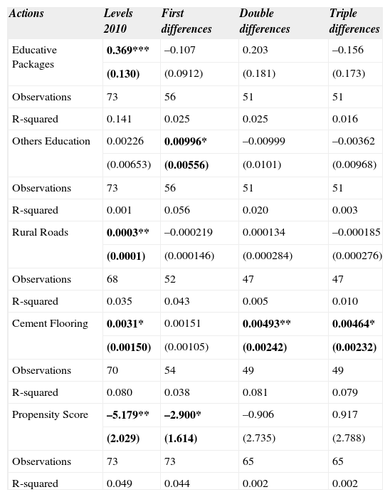
Table 7 shows the results for the Rate of Scholar Attendance from 6 to 24 years old. The results indicated a statistically significant trend on the improvement of the rate of scholar attendance as the level of investment per capita increased for the strategic actions Educative Packages and Rural Roads for the simple difference in 2010, other actions in Education¹¹ for the difference in difference, and Cement Flooring¹² for the simple difference, double and triple difference. Again, this table shows that the improvement in the rate of scholar attendance was greater for those municipalities with greater investment. In other words, what these figures show is that there was a progressively increasing positive effect on the rate of scholar attendance as the level of investment per capita in the actions mentioned above increased.

Table 7.

Matched differences att for scholar attendance.

Actions	Levels 2010	First differences	Double differences	Triple differences
Educative Packages	0.369***	–0.107	0.203	–0.156
	(0.130)	(0.0912)	(0.181)	(0.173)
Observations	73	56	51	51
R-squared	0.141	0.025	0.025	0.016
Others Education	0.00226	0.00996*	–0.00999	–0.00362
	(0.00653)	(0.00556)	(0.0101)	(0.00968)
Observations	73	56	51	51
R-squared	0.001	0.056	0.020	0.003
Rural Roads	0.0003**	–0.000219	0.000134	–0.000185
	(0.0001)	(0.000146)	(0.000284)	(0.000276)
Observations	68	52	47	47
R-squared	0.035	0.043	0.005	0.010
Cement Flooring	0.0031*	0.00151	0.00493**	0.00464*
	(0.00150)	(0.00105)	(0.00242)	(0.00232)
Observations	70	54	49	49
R-squared	0.080	0.038	0.081	0.079
Propensity Score	–5.179**	–2.900*	–0.906	0.917
	(2.029)	(1.614)	(2.735)	(2.788)
Observations	73	73	65	65
R-squared	0.049	0.044	0.002	0.002

Note: The ols regressions were run with robust standard errors and standard errors being the larger errors the ones who are reported in parentheses: *** p < 0.01, ** p < 0.05, * p < 0.1. First difference: (2010-2005); Double differences: 2010-(2005-2000); Triple differences: (2010-2005)-(2005-2000).

Source: Own elaboration.

The results for the heterogeneous treatment effects of the program as a function of the PS to treatment suggested that the improvement in the rate of scholar attendance was larger for those municipalities who were less likely to be part of it.

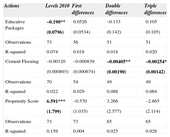
Table 3 presents the results for the Rate of Scholar Absence from 6 to 14 years old. The results were statistically significant and negative for the investment per capita in Educative Packages for the simple difference in 2010 and Cement Flooring for the simple difference of 2010, double and triple differences. This indicated that as the level of investment per capita in each of these actions increased, the estimated impact on the reduction on the rate of scholar absence increased as well. Thus, the expected effect of E100×100 on the Rate of Scholar Absence was larger for those municipalities on which the intervention included financial resources to the municipalities through these specific actions. It is worth mentioning that the specific action Cement Flooring of the Housing Aspect was believed to have an impact on the reduction of the scholar absence as it provided households with better hygienic conditions and therefore reduced the probability of getting sick and skip school.

Table 8

Table 8.

Matched differences att for Rate of Scholar Absence 6 to 14 years old.

Actions	Levels 2010	First differences	Double differences	Triple differences
Educative Packages	–0.190**	0.0526	–0.133	0.105
	(0.0796)	(0.0534)	(0.142)	(0.105)
Observations	73	56	51	51
R-squared	0.074	0.018	0.018	0.020
Cement Flooring	–0.00120	–0.000839	–0.00405**	–0.00254*
	(0.000893)	(0.000674)	(0.00190)	(0.00142)
Observations	70	54	49	49
R-squared	0.022	0.029	0.088	0.064
Propensity Score	6.591***	–0.570	3.266	–2.865
	(1.799)	(1.035)	(2.577)	(2.114)
Observations	73	73	65	65
R-squared	0.159	0.004	0.025	0.028

Note: The ols regressions were run with robust standard errors and standard errors being the larger errors the ones who are reported in parentheses: *** p < 0.01, ** p < 0.05, * p < 0.1. First difference: (2010-2005); Double differences: 2010-(2005-2000); Triple differences: (2010-2005)-(2005-2000).

Source: Own elaboration.

The results of the heterogeneity in the treatment effects of E100×100 as a function of the PS show that the coefficient of the PS was statistically significant and inversely correlated to the estimated effect on the Rate of Scholar Absence. Again, this relationship showed once more a progressively increasing effect, this time on the reduction of the rate of scholar absence, as municipalities with lower PS were included.

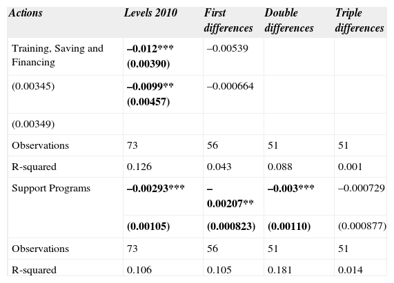
Table 9 illustrates the results for the percentage of households without washing machines. These results indicated that there was a progressively greater effect as the investment per capita in actions of Training, Savings and Financing —in simple and double differences— and Support Programs for Economic Activities —in simple, first and double differences— increased.

Table 9.

Matched differences att for percentage of households with no laundry.

Actions	Levels 2010	First differences	Double differences	Triple differences
Training, Saving and Financing	–0.012*** (0.00390)	–0.00539
(0.00345)	–0.0099** (0.00457)	–0.000664
(0.00349)
Observations	73	56	51	51
R-squared	0.126	0.043	0.088	0.001
Support Programs	–0.00293***	–0.00207**	–0.003***	–0.000729
	(0.00105)	(0.000823)	(0.00110)	(0.000877)
Observations	73	56	51	51
R-squared	0.106	0.105	0.181	0.014

Note: The ols regressions were run with robust standard errors and standard errors being the larger errors the ones who are reported in parentheses: *** p < 0.01, ** p < 0.05, * p < 0.1. First difference: (2010-2005); Double differences: 2010-(2005-2000); Triple differences: (2010-2005)-(2005-2000).

Source: Own elaboration.

Similar results were also found for the percentage of households without refrigerators for the first, double and triple differences in the case of Support Programs and for the double differences for Training, Savings and Financing.

The last tables show the estimated results on Coneval's Multidimensional Measurement of Poverty, variables only available for the year 2010, this being the reason why no estimations are presented under the difference in difference approach.

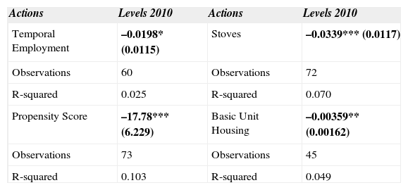
Table 10 shows the results for the percentage of people in poverty due to quality and spaces of the dwelling. This table shows statistically significant and negative coefficients for the investment per capita in the actions of Stoves¹³ Temporal Employment and Basic Unit Housing. That is, a progressively increasing impact was observed as the investment per capita in these actions increased. Again what these figures show is that municipalities with greater levels of investment per capita in these actions experienced a larger reduction in the percentage of people in poverty due to quality and spaces of the dwelling outcome indicator.

Table 10.

Matched differences att for deprived in the quality and spaces of housing.

Actions	Levels 2010	Actions	Levels 2010
Temporal Employment	–0.0198* (0.0115)	Stoves	–0.0339*** (0.0117)
Observations	60	Observations	72
R-squared	0.025	R-squared	0.070
Propensity Score	–17.78*** (6.229)	Basic Unit Housing	–0.00359** (0.00162)
Observations	73	Observations	45
R-squared	0.103	R-squared	0.049

Note: The ols regressions were run with robust standard errors and standard errors being the larger errors the ones who are reported in parentheses: *** p < 0.01, ** p < 0.05, * p < 0.1.

Source: Own elaboration.

The coefficient estimated for the trend in the PS was statistically significant indicating that the municipalities that were more likely to participate in the program were the ones which had the largest improvement in this indicator. A result that contrasted with that of the educational aspect of the program, suggesting the different contexts in which these actions seem to work for the benefit of the targeted population.

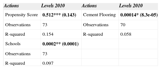
Table 11 presents the results for the percentage of the population not multidimensional poor and not vulnerable. Two specific actions showed a statistically significant trend: Cement Flooring and Schools. As shown in this table, there was a gradually increasing positive effect on this indicator as the level of investment per capita in the actions increased.

Table 11.

Matched att differencesfor not poor neither vulnerable population.

Actions	Levels 2010	Actions	Levels 2010
Propensity Score	0.512*** (0.143)	Cement Flooring	0.00014* (8.3e-05)
Observations	73	Observations	70
R-squared	0.154	R-squared	0.058
Schools	0.0002** (0.0001)
Observations	73
R-squared	0.097

Note: The ols regressions were run with robust standard errors and standard errors being the larger errors the ones who are reported in parentheses: *** p < 0.01, ** p < 0.05, * p < 0.1. Source: Own elaboration.

For the case of the PS, the results suggest that the impacts of the program were largest for those municipalities that had PS close to unity. Meaning that there was a progressively increasing effect of the program as the poorest municipalities were included.

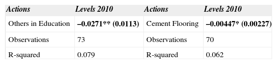
Table 12 shows the results for the outcome variable population with at least three social deprivation indicators. The coefficients for the Cement Flooring and Others in Education actions were statistically significant and negative, which means that the reduction on these outcome variables increased along with investment per capita in these actions.

Table 12.

Matched att differences for population with at least three social deprivation.

Actions	Levels 2010	Actions	Levels 2010
Others in Education	–0.0271** (0.0113)	Cement Flooring	–0.00447* (0.00227)
Observations	73	Observations	70
R-squared	0.079	R-squared	0.062

Note: The ols regressions were run with robust standard errors and standard errors being the larger errors the ones who are reported in parentheses: *** p < 0.01, ** p < 0.05, * p < 0.1.

Source: Own elaboration.

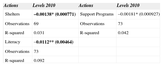
Lastly, in Tables 13 and 14 we see the results for the percentage of population with income below the minimum welfare line indicator and extreme poverty. In Table 13, the investment in three specific actions showed a statistically significant trend: Support Programs for Economic Activities¹⁴, Literacy, and Shelters.

Table 13.

Matched ols differences for population with income below the minimum welfare line.

Actions	Levels 2010	Actions	Levels 2010
Shelters	–0.00138* (0.000771)	Support Programs	–0.00181* (0.000927)
Observations	69	Observations	73
R-squared	0.031	R-squared	0.042
Literacy	–0.0112** (0.00464)
Observations	73
R-squared	0.092

Note: The ols regressions were run with robust standard errors and standard errors being the larger errors the ones who are reported in parentheses: *** p < 0.01, ** p < 0.05, * p < 0.1. Source: Own elaboration.

Table 14.

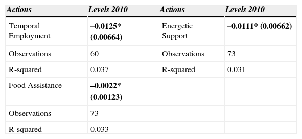
Matched att differences for extreme poverty.

Actions	Levels 2010	Actions	Levels 2010
Temporal Employment	–0.0125* (0.00664)	Energetic Support	–0.0111* (0.00662)
Observations	60	Observations	73
R-squared	0.037	R-squared	0.031
Food Assistance	–0.0022* (0.00123)
Observations	73
R-squared	0.033

Note: The ols regressions were run with robust standard errors and standard Errors being the larger errors the ones who are reported in parentheses: *** p < 0.01, ** p < 0.05, * p < 0.1.

Source: Own elaboration.

In Table 14, the coefficients for the investment per capita in Energetic Support, Food Assistance¹⁵ and Temporal Employment were statistically significant and negative. Indicating again that the municipalities that received the largest amounts of investment on these actions were the ones who exhibited greater reductions of this indicator.

Conclusions

In the pursuit of effectiveness of development policies, the crucial need to coordinate different levels of governments and institutions is not a new topic and its importance is continuously advocated (see Bouckaert, Peters, and Verhoest, 2010; Peters, 2015).

Since the seventies Mexico has ventured in the design of policy strategies oriented at solving the shortcomings left by poor management of interdependencies in development policies. Indeed, the efficiency costs of the lack of coordination and collaboration between players at different levels of government, ministries and program administrators has long been recognized.

Every new administration endorses the need to develop a comprehensive plan to determine and respond to the needs for coordinating processes and procedures among adjacent institutions and between levels of government. However, managing this kind of interrelations has proven an elusive undertaking. Admittedly, this is not an easy task. It is a complex web of interdependencies, simultaneously vertical, across different levels of government, and horizontal, among ministries and programs at the same level of government, and networked (Koliba, Meek, and Zia, 2010). Surprisingly, there is only a handful of studies in Mexico that investigate the tools being used to help bridge the gaps that exist between levels of government as they design and implement public policies (see Collins et al., 2004; Ordaz Ocampo, 2012; Camacho García and Flamand, 2008; Cejudo Ramírez, 2012; Kroeger and Luna, 1992; Yaschine, Ochoa, and Hernández, 2014).

From our part, at the results level, the evidence presented in this paper suggests a positive impact of E100×100 whenever managed to get accompanied by a minimum of investment. Hence, it's possible to give an affirmative answer to the hypothesis that whenever E100×100's intervention included the needed investment per action to the treated municipalities, the expected effects were found. This shows that even though, in the intention-to-treat evaluation carried out by Coneval, it was not possible to find many statistical significant differences, this did not imply that the intervention was not effective. It simply means that the E100×100 couldn’t intervene equally across municipalities. Furthermore, the evidence presented suggests the expected results were observed for those outcome variables whose associated actions successfully secure a minimum of investment.

These findings bring new elements of analysis for the intention-to-treat evaluation done by Coneval indicating that it was less likely that their evaluation did not find the expected effects because the control municipalities ended up being treated. On the contrary, it has been shown that it is more likely that the municipalities in the treatment group actually received different treatments, some more effective than others. In other words, it has been suggested that E100×100's intervention seems to have worked best whenever it managed to get accompanied by a certain level of investment. However, in more cases than not, the E100×100 umbrella program couldn’t go that last mile.

For the actions on which the intervention did not secure a minimum investment, the results were not the expected ones. Again, the important thing to notice is that the evidence provided suggests that the intention-to-treat evaluation did not find many statistical differences because the municipalities in the treatment group actually ended up not being treated differently than the control group in the sense that the intervention did not always include financial resources. Moreover, the evidence presented here poses severe doubts on the hypotheses advanced in the previous evaluation that no significant results were found due to the possibility that some of the municipalities in the control group were also intervened.

What is behind these differences in the treatment received by the municipalities is hard to know without field data. However, it has long been recognized that the interinstitutional coordination is a complex matter and that policy designers face several hurdles to establish common goals and have an efficient communication among the actors involved. Moreover, the task of setting strategic priorities is inherently political and this could also pose several limits to the effectiveness of coordinated strategies (Evans, 1995). It has also been known for a long time now that a key element in the efforts to develop an efficient and sustainable coordination of public service delivery is the existence of a series of formalised measures, mechanisms and steps that ensure the commitment in the activities that need to be carried out by the actors involved in coordination process (Grindle, 2010; North and Shariq, 2004; Ordaz Ocampo, 2012). An element missing in the original design of E100×100.

Hardly anyone would contest the importance of competent and committed individuals with strong values, good judgment and sound knowledge and understanding of the mutual dependence of policy responsibilities behind it all. However, without the management basis for the entire interinstitutional coordination plan, a document that establishes committees and policies placing responsibility and authority where they are needed to accomplish tasks, there is little hope even for otherwise well-intentioned officials to overcome the natural resistance of competition and turf protection (Yaschine, Ochoa, and Hernández, 2014).

Thus, the Mexican government needs to start taking actions in order to develop and implement the formal mechanisms that represent a challenge for the interinstitutional coordination. The mechanisms should focus on the clear recognition of the existing government conditions and capacities to set and implement feasible priorities in a strategic manner. There is a need for clarity in roles, responsibilities and objectives. The need to focus on the specific requirements of the communities in which services are delivered is apparent. The search for diverse methods to ensure accountability and the creation of regulatory frameworks or agreements for collaboration to take place are a must. A strong national leadership and management is required to strengthen both local government and civil society. The encouragement of participation between communities and institutions to provide local solutions to local issues, along with regular meetings and effective communication among the representatives from many different ministries and agencies across government and the investment of time and resources into community consultations and consensus building are needed (Keast, 2011; Stewart, Lohoar, and Higgins, 2011; Grindle, 2010; Gray, 2002; Leigh, 2008; Grindle, 2004; Ordaz Ocampo, 2012; Sabatier, 1986).

As long as the Mexican government continues assigning economic resources to programs like the E100×100 without creating the necessary conditions mentioned above, any further attempts such as the recent Cruzada Nacional Contra el Hambre [National Crusade Against Hunger] launched by the current administration will continue most likely to not show the desired results. Nowadays, Coneval has commissioned a specific assessment of the interinstitutional coordination processes and procedures behind Cruzada Nacional Contra el Hambre, a program that certainly left things to be desired from the start (Yaschine, Ochoa, and Hernández, 2014). The results of which, expected by 2016, will likely point in the same direction.