


This article deals with mathematical models for controlling vehicles behavior in a virtual world, where two behaviors are considered: 1) curve turning and 2) car following situations, in this last is essential to provide a safety distance between the leader and the follower and at the same time keep the follower not delayed with respect to the leader, and in a curve turning the complexity is to provide a safety speed inside the curve and keep the car inside the lane. Using basic information as vehicles position, mathematical models can be developed for explaining the heading angle and the autonomous vehicles speed on curves, i.e. the controlled by the models. A model that predicts the autonomous vehicle speed on curves is developed considering previous data in other curves. Two models that control the acceleration/deceleration behavior of autonomous vehicles in a car following situation are proposed. In the first model, the parameters are calibrated with a proposed algorithm which enables accuracy in order to imitate the human behavior for accelerating and braking, and the second model provides a safety distance between the follower and the leader at sudden stops of the latter and employs the acceleration/deceleration top capabilities to follow the leader car similar to the human behavior.
Este artículo introduce modelos matemáticos para controlar el comportamiento de vehículos en un mundo virtual; estos comportamientos consideran dos situaciones: 1) en toma de curvas, donde la complejidad es resultado de mantener al vehículo a una velocidad segura durante la toma de la curva y dentro del carril y 2) de seguimiento vehicular, donde es esencial mantener una distancia segura entre los vehículos, así como evitar que el vehículo seguidor quede rezagado con respecto al líder. Usando información básica sobre la posición de los vehículos se desarrollan modelos matemáticos que explican el ángulo de dirección y la velocidad en curvas de vehículos autónomos. Se desarrolla un modelo para predecir la velocidad del vehículo autónomo en curvas considerando datos previos en otras curvas. Se proponen dos modelos para controlar el comportamiento para acelerar y desacelerar de los vehículos autónomos en situaciones de seguimiento de coche, el primer modelo se calibra con un algoritmo propuesto y asemeja el comportamiento humano para acelerar y frenar, el segundo proporciona una distancia segura para evitar colisiones cuando el líder frena repentinamente, además emplea la máxima capacidad para acelerar y desacelerar del vehículo autónomo y asemeja el comportamiento humano.
The car following situations had been studied over the years because its importance in understanding and predicting the human behavior to accelerate and brake. A historical review of the models that describe this phenomenon is presented in Brackstone & McDonald (1999), where it can be seen the car following model proposed by Gazis et al. (1961), called GHR, with formula where af is the car following acceleration, is the car following speed, Δv and Δx are the relative speed and distance between the leader and the follower, c, m and l are the model parameters. Ceder & May (1976) found the parameters values for congested and uncongested traffic using a larger set of data and concluding that the data is fitted better using two regimens. Treiterer & Myers (1974) split the GHR model in two phases, when the vehicle accelerates or decelerates. Recently in Ma & Andréasson (2006), the reaction time, i.e. the time required by the driver to respond, is estimated and used in the nonlinear General Motor model. The reaction time is calculated analyzing data in the frequency domain through Fourier transform and spectrum analysis, then with the estimated reaction time the parameters of the model are calibrated, the data used for calibration is taken from the stable following regime. In Ranjitkar et al. (2005) an optimization considering a genetic algorithm is implemented in order to calibrate car following models, some of these are the Chandler, Gipps, and Leutbach models, the results of their work are the mean and standard deviation of the models parameters optimum values.
In relation with the vehicle speed on curves, it becomes important to consider the curve design and the vehicle behavior in order to implement speed predictions. In Zhang et al. (2013) an algorithm based on a recursive least square method with a forgetting factor is employed to calibrate their model, employing as independent variables the vehicle velocity at the entrance of the curve, the road curvature and two regression coefficients, these variables are adjusted for representing a particular user driver behavior. In Wolfermann et al. (2011) a model that describes the vehicle speed at intersections is presented, including vehicle turning to right and left, where it was observed that when a vehicle is turning decelerates until a minimum speed is reached, after this accelerates to the desired speed. The profile is explained by the model in two parts, the inflow and outflow, separated by the point when the minimum speed is reached. The model is presented as a polynomial of third degree where the dependent variable is the turning speed and the independent variable is the time, the coefficients are calibrated for the inflow and outflow cases. Considering the speed that a vehicle will maintain on a curve, in Abbas et al. (2011) an equation for predicting the 85th percentile operating speed on horizontal curves through multiple linear regression analysis is presented, where the inverse square root of the radius curve and the 85th percentile speed at approach tangent result as significant variables to explain that 85th speed.
Two mathematical models are proposed in this article to control the autonomous vehicles in car following situations. The models simulate the behavior of a vehicle that is following another vehicle in the next front called leader vehicle, so that the behavior of the follower is strongly related with the leader. The first model is designed to describe the human acceleration/deceleration behavior and its parameters are calibrated to represent a particular behavior driver, e.g. a moderate or aggressive driver, or employing data of different users, calibrated to represent a general behavior. The second model represents a specific case, the acceleration of the following car is calculated so that its speed is smoothed to reach the leader vehicle's speed according a calculated distance and this last depends on the actual velocity and acceleration of the follower and leader.
The other contribution is the explanation of the autonomous vehicle speed when it enters on a curve until the desired speed is reached, using the time as the independent variable, the speed is obtained with a regression equation employing a least square technique. Subsequently, based on a pattern observed between a coefficient of the reduced degree speed equations and the radius on different curves, the turning speed is predicted for a set of curves. Additionally, the vehicle's desired speed on a curve is explained, i.e. when the vehicle reaches the safety speed that will be maintained during the rest of the curve. In order to explain this behavior, the radius curve size, and the time to reach the safety speed are used as independent variables, the equation is obtained using data from a set of curves and tested in another set obtaining positive results about its prediction capability.
The article is organized as follows: the method section presents the equations employed in the conducted tests as well as the form of the proposed models. The models that control the acceleration/deceleration of the autonomous vehicles and the experimental vehicle –controlled by the user– in a car following situation and the model that describes the turning speed are presented.
The experiments and discussion section presents the comparison results between the first proposed car following model and the general motors (GM) model, in addition to the experiments to test the accuracy of the second proposal model. In addition, the results of the models that control the heading angle and the speed of the autonomous vehicle during a turning maneuver are included, as well as the results obtained with the proposed model to predict the comfortable (or safe) speed in a curve. Finally the conclusions are drawn considering the contributions obtained.
MethodIn this section, the mathematical models to set the acceleration and deceleration of the user controlled vehicle and the autonomous vehicle in free driving conditions are presented, also the proposed models in car following situations.
Leader car acceleration and deceleration modelsFor simulation purposes, in the particular case of car following situations, i.e. when the behavior of a car is related to a car right in front, is required to control the acceleration of both cars using a model for each one, an example from the simulations of a car following situation can be observed in Figure 1.

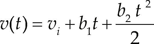
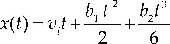
The model selected for setting the acceleration of the leader car is called polynomial model, explained in detail in Akcelik & Biggs (1987), the model is presented in Equations 1 and 2 that calculates the acceleration and speed, respectively.
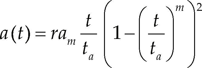
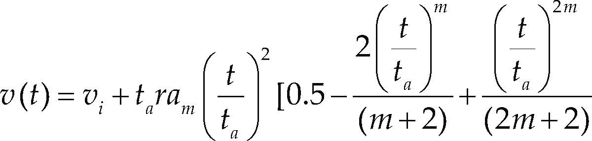
Where r and m are model parameters, am is the maximum acceleration, and ta is the acceleration time, i.e. the time required to reach the final speed. The initial vi and final speed vf are employed to approximate the acceleration time with Equation 3.

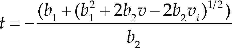
In the case for decelerating the leader car the same model presented in Equation 1 is employed, explained in Akçelik & Besley (2001), with the variant that instead of ta, td the required time to reach a zero final speed, is estimated with Equation 4.
Proposed models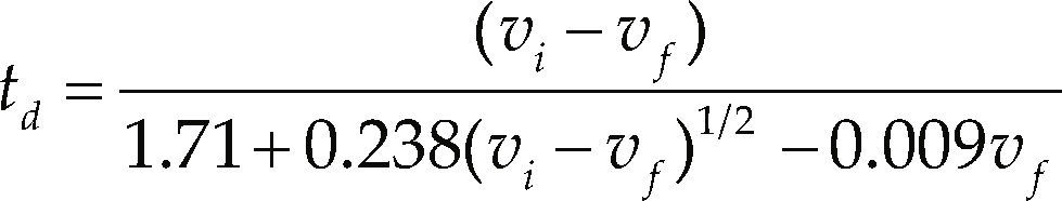
The first proposed model simulates the driver behavior in car following considering two situations: 1) when the leader car speed vl is greater than the following car speed vf, i.e. vl > vf, and 2) in the case where vl < vf. In the first case, the model presented in Equation 5 is proposed for setting the acceleration of the following vehicle
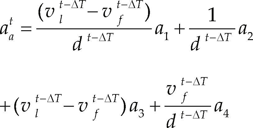
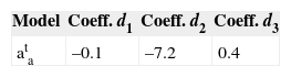
where d is the distance between the leader and the following car, measured from the centers of the cars, the parameters of the model are a1, a2, a3 and a4, and ΔT = 1 is the reaction time, i.e. the time that the driver needs to react. In the second case, the deceleration of the following vehicle is presented in Equation 6,
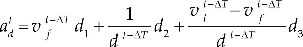
where d1, d2 and d3 are parameters. The models form Equations 5 and 6 are calibrated according to a proposed algorithm called parameter estimator, which consists in finding the best parameter value inside a range, the calibration of the parameters is conducted in the order of appearance in the model, i.e. following the parameters subscript numerical order. In order to calibrate the first parameter the others are set in zero and a parameterized search is performed of the parameter value that reduces the error model. The next parameter is calibrated in the same way but keeping the previous parameter value as it was tuned, and so on, until all the parameters are calibrated. The annex presents the coefficient values obtained for the acceleration and deceleration cases. The algorithm is presented next, where N is the number of parameters, linf = –20 and lsup = 20 are the inferior and superior limits defined in the search field (these limits were found suitable for the experiment cases), the model function to calibrate could be equation 5 or 6, oi is the observed data of size j, the output yn is the parameter value with the minimum error. The case for calibrating equation 6 is presented in algorithm 1.
Algorithm 1.Parameter estimator algorithm (PEA)
After the acceleration or deceleration is calculated, the speed is obtained with the Newton's law of motion, discretized in time and presented in Equation 7, where Δt » 0.2s is the step simulation time.

The second model proposed simulates the acceleration/deceleration human behavior according the form of the double sigmoid, see Figure 2; the proposed model extrapolates the leader vehicle speed using four samples behind with a polynomial of third order to predict the distance between the vehicles to be used in the calculus required by the model.

The acceleration of the following car is rigged by Equation 8, in which the parameters S, R and A will modify the aggressiveness to approach the leader and the distance between them.

R is the ratio between the safety distance dS and the actual distance d between the leader and the following car minus a minimal distance dm, this last should be at least the car size plus one meter in order to avoid collisions, a similar use of Equation 9 in a different context (to control a robotic arm movements) can be found in De Jesús et al, 2014).
A is the maximum acceleration or deceleration that can be applied by the vehicle, defined in Equation 10.

S is the aggressiveness of the acceleration and deceleration changes, being a positive value. If 0 ≤ S < 1 make it smoother, and 1 ≤ S < ∞ make it less smoother, S is selected as presented in Equation 11, allows reacting at sudden changes of the leader velocities.

The safety distance dS is calculated in Equation 12, where the second term allows the following car to react to the next position data rate and gives an extra space to avoid collisions,
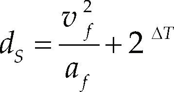
where af and vf are the acceleration and speed of the following vehicle and ΔT is the time step at which the status of the leader vehicle is obtained.
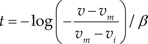
Experimental vehicle acceleration and deceleration modelsThe experimental vehicle is the controlled by the user through the keyboard in the Virtual World, the model that set its behavior for accelerating is explained in detail in Ramsay (2007) as well the procedure for calibrating the parameters. The acceleration model and their integrals are presented in Equations 13, 14 and 15.
with b = α/vm, being α the maximum acceleration, vm the maximum speed, β the rate at which decreases the acceleration respect the speed, and vi is the initial speed. The time can be solved manipulating Equation 14,


To decelerate the experimental vehicle, a linear model is used, the model and their integrals are presented in Equations 17, 18 and 19.
where b1 is the maximum deceleration and b2 is the rate at which the deceleration decreases respect time, b1 is the maximum deceleration that can be applied, b2 is calibrated with Equation 20.where td is the time when v = 0, td can be calculated with Equation 4. From Equation 20 the time can be solved.Vehicle behavior on curves

The behavior of the experimental vehicle when it enters in a curve is explained, where the dependent variables are heading angle and speed, and the independent variables are in the time and the vehicle position coordinates. The variables chosen for describing the heading angle of the vehicle in curves are the coordinates of the vehicle position in a three dimensional coordinate system; however, in the explanatory equation the axis normal to the plane is omitted because in the contemplated cases the vehicle has no movement in that axis.
To set the degree of relationship between the dependent and independent variables of the proposed models the coefficient of determination is needed. A mul- tiple regression using the least squares method is used to explain the heading angle using the coordinates of the vehicle position, the speed is explained using the time with a polynomial regression.
Experiments and discussionThe Virtual World created in order to implement the experiments was developed in the Unity engine; the data employed was obtained from user tests. In the vehicle turning tests cases, it is considered that the vehicle enters the curve an approximated speed of 60km/h, and there is no influence of other vehicles in the front or back. The created curves represent one quarter of the circle circumference since the vehicle reaches the comfortable speed before completing the circle circumference quarter. In order to obtain data in car following situations the leader vehicle accelerates gradually from zero to the maximum acceleration and then smoothly returns to cero, the same for decelerating; in the case of the following vehicle, i.e. the vehicle controlled by the user, it accelerates linearly from the maximum acceleration to zero and the same way for decelerating. The tests to obtain the data are performed as follows: first the vehicles –leader and follower– as initial conditions are stopped, then the leader accelerates and the follower begins to follow it until both enter in a stable regime, after that the leader begins to decelerate and the follower does the same until both vehicles are stopped.
Construction of the curve roadsThe scenarios of the Virtual World which were employed to implement the experiments conducted in this article, were created in the Unity engine as well the vehicles and roads; nerveless González & Arámburo (2013) present a method that allows the construction of the linear and curve roads where a vehicle equipped with a simulated GPS has circulated, i.e. the vehicle position coordinates are obtained.
Car following experimentsThe proposed models in Equations 5 and 6 were tested with different data that the used for calibrating their parameters, all the data were obtained with the leader car using the acceleration and deceleration model of Equation 1, the following car is controlled by the user as the experimental vehicle, using the model for accelerating presented in Equation 13 and for decelerating in Equation 17. The results obtained with the proposed model are compared with the General Motors model, this last detailed in Mathew & Krishna (2007). Table 1 shows the mean absolute error (MAE) obtained with the proposed and the GM models, this last calibrated with the algorithm proposed in this article employing the same data as the used for calibrating the proposed models. As can be observed in Table 1, there is an improvement in the acceleration and deceleration phases with respect to the GM model.
The equation employed to obtain the mean absolute error is presented in Equation 22, where oi is the observed value, mi is the modeled value, and n is the total number of observations.
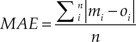
Figure 3 depicts the observed vs predicted acceleration and Figure 4 shows the observed vs predicted deceleration, each graph for the corresponding model presented in Table 1.


The proposed model in Equation 8 was tested for behavioral analysis using a typical configuration of the car with 4 m/s2 (14.4km/h/s) for maximum acceleration and –4.5 m/s2 (–16.2km/h/s) for maximum deceleration, ΔT varies and is the time step at the obtained vehicles position coordinates. In Figure 5, the leader car is 200 meters from the follower, then we observed the variables –acceleration, velocity and distance– of the follower to reach the leader, with ΔT = 1s and applying extrapolation between the intervals of time. Figure 6 presents the case considering ΔT = 0, i.e. the data of the leader is used at the time step at which the simulator is running, in this case, extrapolation results redundant. The leader car departs from 0 to 80km/h and employs the model presented in Equation 1. The units of the plots from here to the end of the subsection are distance in meters, velocity in km/h and acceleration in km/h/s, the horizontal axis shows the time in seconds.


In Figure 7 we can observe the behavior of the following car for a test where the leader starts moving from 0 to 80 km/h and decelerates to a complete stop, the initial distance between the vehicles was 11.14 m, with ΔT = 1s and extrapolating. The test is conducted in the same way without extrapolation with the results in Figure 8, where it can be observed the acceleration abrupt changes.


In Figure 9 we observed the following behavior when the leader car suddenly stops, with ΔT = 1s and extrapolating. The same test was performed with the following car using the GM model with the parameters values suggested by Ozaki (1993), whith α = 1.1, m = –0.2 and l = .2 for accelerating, and α = 1.1, m = 0.9 and l = 1 for decelerating, results are presented in Figure 10, where it can be observed that the following vehicle needs to apply a maximum deceleration of –41.1621km/h/s (which gradually decreases) that exceeds the proposed limit of –16.2km/h/s.


Figure 11 presents the extreme case with ΔT = 5 s and the leader going from 0 to 80km/h; then gradually decelerating until it is at rest. It can be observed that the extrapolation procedure maintains a more realistic behavior than without extrapolating, as in Figure 12.


In the next experiment a second follower car is introduced, both followers are working with the proposed model in Equation 8; in Figure 13 it can be observed the behavior of the first follower with ΔT = 1 s and the leader going from 0 to 80km/h and then gradually decelerating, Figure 14 presents the speed and acceleration of the second follower.


The behavior of the first follower at a sudden stop of the leader going at 80km/h is presented in Figure 15, Figure 16 shows the second follower behavior, the experiment with ΔT = 1 s.
Heading angle model

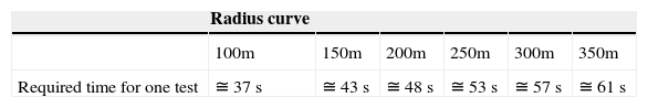
The data employed to calibrate the heading angle model are obtained driving the experimental vehicle on curves with different radius sizes, the experiments were conducted on curves with radius in the size range 100 ≤ r ≤ 200, with r being the radius. The driving results are plotted until the desired speed is reached, Figure 17 shows the case of a curve with a radius of 100 meters and the x coordinate vs heading angle, Figure 18 shows time vs speed.


The coordinate where the curve begins is denoted as (xc, yc), this location is used to conduct all the experiments involving curves, where (xc = 4246.52, yc = 350). The results presented in this article can be replicated in any coordinate system by translating the origin of the curves to (xc, yc).
Figure 17 shows that the vehicle begins with the heading angle θ = 0 and moves from right to left. In Figure 18 the vehicle speed is decreasing as the time increases, the speed became constant at approximately t = 5.5 s, i.e. when the desired speed is reached. With the data obtained from the tests the model that relates the heading angle with the position is obtained, subsequently with the vehicle position the time is explained, finally the model that explains the speed on curves with time as the independent variable is obtained. Three tests for each curve were conducted, Table 2 presents the approximate required time for each curve test.
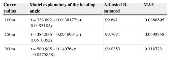
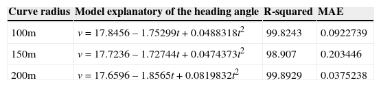
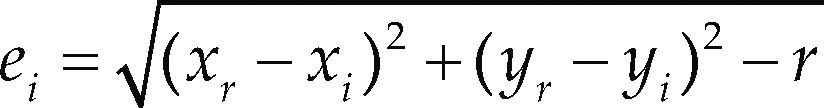
Table 3 presents the models that explains the heading angle of the vehicle in a curve, together with statistical results –adjusted R-squared and MAE. With the objective to test the accuracy of the models presented in Table 3, an autonomous vehicle with a fixed speed of 10 m/s is provided with the corresponding model for each curve case, the trajectory is measured and it is verified that the vehicle stays inside the lane. The case of a curve with a 100 m radius is presented in Figure 19, where the autonomous vehicle trajectory is presented in red and the lane borders in black, the lane width measure is 7.5 m for all the experiments. The trajectory —100 m radius case—, presented in Figure 20, is measured according the Euclidian distance between the origin of the curve (xr, yr) and the points obtained from the vehicle trajectory (xi, yi) minus the radius size, since the width of the lane is 7.5 m and the autonomous vehicle measure 2 m of width and 4 m of length, the permissible distance to avoid leaving the lane is a displacement of 2.75 m from the center of the lane, the equation to obtain the error is Equation 23.
Heading angle explanatory equations.
| Curve radius | Model explanatory of the heading angle | Adjusted R-squared | MAE |
|---|---|---|---|
| 100m | θ = 41388.8 – 19.4245x + 0.529775y + 0.00226879x2 | 99.752 | 1.01345 |
| 150m | θ = 1467.69 – 0.41270x + 1.24124y – 0.00122387y2 | 99.8492 | 0.749063 |
| 200m | θ = 17533.6 – 8.39754x + 0.00100239x2 + 0.000409264y2 | 99.8908 | 0.674053 |


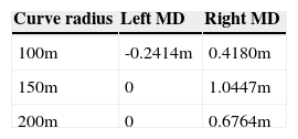
Table 4 contains the left and right maximum displacements (MD) of the autonomous vehicle from the center of the curve, the vehicle circulates according to the model of their respective curve. Figure 21 shows an example of a vehicle taking a curve.

The coordinates of the vehicle position on a curve are used as the independent variable to explain the time, see Table 5. The time is employed as the independent variable for explaining the turning speed of the autonomous vehicles, observe Table 6. Figure 22 presents the x coordinate vs. the modeled angle and the observed angle from tests, Figure 23 shows the time vs. the modeled speed and the speed from tests, in both cases for a radius curve of 100 m as example.


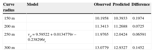
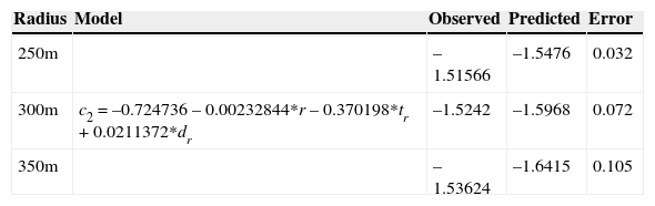
The speed obtained from equations in Table 6 is employed until the desired speed va is reached; this speed can be explained considering two independent variables, the radius of the curve and the time tr to reach the desired speed starting at the beginning of the curve. The model to predict the desired speed was calibrated considering data with curve radius of 100 m and 350 m, obtaining an adjusted R-squeared of 99.6859. In order to find if the model can predict the desired speed, the tests were conducted in a radius range 150 ≤ radius ≤ 300 for four cases, the model is presented in Table 7 with the difference between the average of the observed desired speed in that curve and the one predicted by the model. In order to predict the coefficients of the model that explains the speed from the beginning of the curve until the desired speed is reached, the order of the equations obtained in Table 6 is reduced, resulting in Table 8. It can be observed in this table that the coefficient of the independent variable decreases as the radius increases. The model that explains the coefficient of the independent variable of the curve speed model of Table 8 is presented in Table 9, where it was obtained an adjusted R-squared of 82.5343 and was calibrated in the range 100 ≤ radius ≤ 200 and tested in a range 250 ≤ radius ≤ 350, being the radius, the time tr and the distance dr traveled until the desired speed is reached, the variables used to explain the coefficient c2.
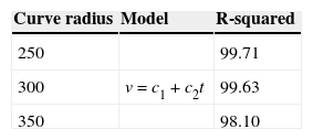
Table 10 contains the equivalent model in Table 8 where the coefficient c1 is determined as the average entrance speed of the tests for each curve case, the second coefficient c2 is obtained with the model in Table 9, then the r-squared obtained for three cases is presented. The observed data is compared with the model that predicts the turning speed using the coefficient obtained in Table 9. Figure 24 shows the time vs the observed and modeled speed for a 250 m radius curve, the same as in Figure 25 for a 300 m radius curve.


The first model presented to control the behavior of the autonomous vehicle in car following situations simulates with accuracy the behavior of the user whose data was used to calibrate the parameters, nerveless it can be calibrated to represent behaviors of different users (e.g. aggressive, passive). A calibration in real time can be performed if data of the desired behavior is available. The proposed model explains two situations of interest in a car following regime, when the following car is accelerating to reach the speed of the leader car and when decelerates if the leader speed is decreasing; in the second case a significant improvement was obtained compared to the GM model.
The second car following model describes the human acceleration behavior using the double sigmoid function to shape the acceleration, and uses the maximum capacity to accelerate and decelerate the following vehicle keeping a safety distance with the leader, that allows the following vehicle to avoid a crash if the leader vehicle brakes suddenly. Another contribution is that extrapolating the speed of the leader –simulating the case when data is not available– the modeled acceleration/deceleration is smoothed but this last decreases as the time delay increases. The case that incorporates a second following car that results in the behavior expected in order to follow the first follower at normal conditions and at a sudden stop of the leader.
The equations that explain the heading angle of the autonomous vehicle in a curve are developed with the information of a vehicle position –simulating GPS data– that already has circulated in that curve, therefore can explain the heading angle that the autonomous vehicle should follow in order to drive in that curve. The experiment results, using the modeled equations, show that the autonomous vehicle circulates in the curves and stays inside the limits of the lane, where a displacement of 1.0447 m was the worst case registered with a tolerance of 2.75 m, i.e. the 37.98% of the available tolerance was used.
The turning speed model, developed to describe the speed of the vehicle since it enters in the curve, explains in the worst case in 98.907% the dependent variable –the speed in the curve. The model implemented to predict the vehicle speed on a curve by estimating the coefficient of the independent variable explains at least in 98.10% the dependent variable. The desired speed on a curve is explained with a model that was tested on different curves than the used to obtain it, resulting in a maximum discrepancy with the expected result of 1.93% and a minimum of 0.55%.
Future workAs future work is pretended to construct a part of the Guadalajara city in a Virtual World, in which autonomous vehicles, controlled with the models presented in this article, will simulate the traffic of the city, so that a vehicle controlled by a person can drive through the virtual city, where the user may experience realistic traffic conditions. In addition the user could improve his traffic skills from an environment with traffic similar to the real one.
AnnexUsing the parameter estimator algorithm (PEA) the coefficients in Tables 11 and 12, that correspond to the models in Equations 5 and 6, are calibrated. According to the PEA in step 1 the search field of the parameter under calibration is defined; Figures 26 and 27 show the coefficient value (CV) which minimizes the error model, this is achieved through step 2, where the model under consideration is evaluated with the coefficient taking values from linf to lsup, in each case the mean absolute error is calculated and the CV that minimize the error is selected, finally step 3 returns to step 1 until all the parameters are calibrated.


Citation for this article:
Chicago citation style
Carrillo-González, José Gerardo, Jesús Arámburo-Lizárraga, Ricardo Ortega-Magaña. Modeling the turning speed and car following behaviors of autonomous vehicles in a virtual world. Ingeniería Investigación y Tecnología, XVI, 03 (2015): 391-405.
ISO 690 citation style
Carrillo-González J.G., Arámburo-Lizárraga J., Ortega-Magaña R. Modeling the turning speed and car following behaviors of autonomous vehicles in a virtual world. Ingeniería Investigación y Tecnología, volume XVI (issue 3), July-September 2015: 391-405.
José Gerardo Carrillo-González An electronic engineer (ITD) with a master degree in sciences (UASLP), has experience in acquisition and data analysis in real time, resolving inverse and direct kinematic issues in robotics. Actually he is in a PhD (UDG) in the area of information technologies, working in the development of mathematical models to control the behaviors of autonomous vehicles in a simulator implemented in a virtual world.
Jesús Arámburo-Lizárraga Received the B.Sc. degree in computer sciences from the Universidad Autónoma de Sinaloa, México, in 2002, and the M.Sc. and Ph.D. degrees from the CINVESTAV Unidad Guadalajara, México, in 2005 and 2009, respectively. Currently, he is Professor at the University of Guadalajara at CUCEA. His research interests include Petri net based fault detection and location of discrete events, distributed systems, and videogames development methods.
Ricardo Ortega-Magaña Computer engineer with a master degree in Electronic and Computer science, with knowledge and experience designing microprocessor and peripherals for embedded systems. Actually he is in developing a multihardware architecture cloud platform to obtain his PhD degree in the Information Technologies field.