Uncertainty spillover and policy reactions

Abstract

Spells of uncertainty are argued to cause rapid drops in economic activity. Wait and see behavior and risk aversion in combination with other frictions can make periods of increased uncertainty an important driver of the business cycle. Emerging economies may endure even stronger and prolonged recessions following a global uncertainty shock, as credit constraints in shallow financial markets limit smoothing. Active policy responses often exacerbate the cycle. The present study uses a novel proxy of uncertainty – inspired on Jurado et al. (2015) – in which I extract a common factor that is not driven by the business cycle from a broad set of forecast indicators. I then estimate an interacted panel VAR on a large set of developed and emerging economies over the period 1990Q1-2014Q3 to test responses to shocks to uncertainty. Emerging markets suffer a larger fall in consumption and investment as uncertainty spreads globally. The main finding is that more developed financial markets are key to dampen the transmission of the shock. Fiscal policy is an alternative, but only if there is sufficient fiscal space to smooth shocks. Monetary policy dampens the effects of uncertainty under a fixed peg better than in a floating exchange rate regime.

Resumen

Se argumenta que los episodios de incertidumbre causan caídas aceleradas de la actividad económica. Los comportamientos de «esperar y ver» y de aversión al riesgo, junto con otras fricciones, pueden originar que los periodos de incremento de la incertidumbre se conviertan en impulsores importantes del ciclo económico. Las economías emergentes pueden padecer las recesiones más fuertes y prolongadas que se producen tras un choque de incertidumbre global, en la medida en que las restricciones al crédito en los mercados financieros superficiales limitan el suavizamiento. Las respuestas de política activas exacerban a menudo el ciclo. El presente estudio utiliza un indicador novedoso de la incertidumbre – inspirado en Jurado et al. (2015) – en el que se extrae un factor común no impulsado por el ciclo económico, de un conjunto amplio de indicadores de pronóstico. A continuación se estima un VAR de panel interactuado para un amplio conjunto de economías desarrolladas y emergentes durante el periodo 1990Q1-2014Q3, con el propósito de probar las respuestas a los choques a la incertidumbre. Los mercados emergentes sufren mayores caídas de consumo e inversión a medida que se expande la incertidumbre a nivel global. El principal hallazgo es que los mercados financieros más desarrollados son esenciales para amortiguar la transmisión del choque. La política fiscal es una alternativa, pero únicamente si existe suficiente espacio fiscal para suavizar los choques. La política monetaria amortigua mejor los efectos de la incertidumbre cuanto existe un tipo de cambio fijo, en comparación a los regímenes de tipo flotante.

1

Introduction

Spells of uncertainty on economic or political events are argued to be responsible for rapid boom-bust patterns in economic activity. “Wait and see” behavior makes agents subject to fixed costs or partial irreversibilities so they keep consumption and investment decisions on hold, only to resume decision taking once the uncertainty is resolved (Bernanke, 1983). Uncertainty also induces risk-averse agents to ask higher risk premia as they fear probabilities of default go up (Arellano, Bai, & Kehoe, 2010; Gilchrist, Sim, & Zakrajšek, 2014). Investors drop projects if they feel that tighter financial constraints make investment temporarily too costly to start up. Recent advances in DSGE modeling techniques show how uncertainty – modeled as a rise in conditional volatility – can be an important driver of the business cycle, especially in combination with other frictions that create some rigidity (see Fernández-Villaverde, Guerron-Quintana, Rubio-Ramirez, & Uribe, 2011).

Emerging economies may endure even stronger and prolonged recessions following a global uncertainty shock, as credit constraints in shallow financial markets trigger stronger responses. Firms are forced to cut back on investment as the financial system withdraws credit lines. Moreover, policy-makers might have trouble to stabilize the cycle if external finance suddenly dries up. This is particularly complicated if erroneous past policy choices put a brake on fiscal policy's intertemporal smoothing if fiscal space is limited. For monetary policy, a trade-off between exchange rate flexibility and the possibility to run an autonomous monetary policy is not obvious for small open economies (Klein & Shambaugh, 2008).

Spells of uncertainty are a latent stochastic process, and must be proxied for by some indicator. The empirical literature has gauged uncertainty from the volatility of financial indicators (Bloom, 2014; Bekaert, Hoerova, & Duca, 2013), cross-sectional dispersion of firm profits or productivity or the disagreement between professional forecasters (Rich & Tracy, 2010; Rossi & Sekhposyan, 2015), dispersion in business and consumer surveys (Bachmann, Elstner, & Sims, 2013), or a measure of keywords in newspapers related to uncertainty (Alexopoulos & Cohen, 2015; Baker, Bloom, & Davis, 2016). The underlying idea of all indicators is that spells over which opinions on financial markets, politics, and the economic outlook are more diverse, are reflecting greater uncertainty.

Empirical evidence seems to concur on the negative effect of uncertainty on economic activity. Uncertainty makes investment drop quickly, with a rebound later on. VAR studies show that consumption is dragged down for longer periods. Similar dynamics are observed in many other G7 countries (Gourio, Siemer, & Verdelhan, 2013). In emerging markets, the effects of uncertainty are found to be much stronger (Carrière-Swallow & Céspedes, 2013; Cerda, Silva, & Valente, 2016).

Some argue that uncertainty is the symptom, rather than the cause of the business cycle. Fluctuations in economic growth shake investment decisions by firms, and a rescheduling of consumption plans by households. Policy-makers must understand the causes and nature of the cycle to stabilize the economy, but are guided by incomplete information at the time of decisions. VAR studies circumvent the problem by arguing uncertainty proxies affects the economy directly, but the measure is not affected by economic developments in the short term. Evidence by Stock and Watson (2012) or Cesa-Bianchi, Pesaran, and Rebucci (2014) puts in doubt this assumption. The present study uses a novel proxy of uncertainty – inspired on Dovern (2015) and Jurado, Ludvigson, and Ng (2015) – that accounts for endogeneity to the business cycle. I employ the Consensus Economics monthly forecasts covering over 480 forecasters in G7 economies on a range of economic projections to extract forecastable projections using a common factor model. As the proxy spans a broad range of economic series and countries, the series is covering economy-wide uncertainty across the globe. As in Henzel and Rengel (2013) or Dovern (2015), I find that the main factor driving forecast errors is correlated with business cycle conditions, and hence is actually forecastable. The measure of uncertainty is the remaining variation in the factors once this cyclical factor is removed.

I then compare the effects of this new uncertainty measure on the economy with standard proxies from Baker et al. (2016) or Jurado et al. (2015). Following Bloom (2009), I estimate the response of investment and private consumption using a panel VAR on a large set of 50 developed and emerging economies over the period 1990Q1-2014Q3. Identification is achieved by cholesky ordering. I condition the VAR estimates on a set of economic characteristics, and examine their interaction with fiscal and monetary policy decisions, following the approach in Towbin and Weber (2013).

Emerging markets suffer larger falls in consumption and investment as uncertainty spreads globally. However, the dynamics of transmission effect do depend on structural characteristics. Countries with more developed financial markets manage to dampen the transmission of the shock as the credit channel allows absorption of the shock. The role of financial markets is much more important than a well-diversified export sector to withstand uncertainty. The recessionary impact is significantly dampened if fiscal policy avoids being procyclical. A country that has sufficient fiscal space can stabilize uncertainty shocks, even if financial markets are shallow. Monetary policy can dampen the effects of uncertainty better under a fixed exchange rate peg than with a floating currency, regardless of economic structure or deepness of financial markets.

These results give support to DSGE models of uncertainty on financial markets in small open economies as in Fernández-Villaverde et al. (2011). Limited access to finance domestically forces agents to borrow abroad. Increased uncertainty on the rates at which to borrow aggravates the economic situation if either fiscal policy – through borrowing on international bond markets – or monetary policy – through interventions on the foreign exchange market – cannot stabilize the economy. For policy-makers, it suggests that stability-oriented monetary and fiscal policy actions – like a peg, or budget control – can alleviate the impact of credit constraints. The impact of uncertainty shocks in these economies would be amplified if policy becomes too activist.

The paper is structured as follows. Section 2 of the paper develops the new multivariate global measure of uncertainty. Section 3 then presents the interacted panel VAR model and discusses the effects on emerging markets of spells of uncertainty, and demonstrates how the responses depend on structural factors and policy responses. Section 4 discusses the implications of our findings for theoretical models and policy-making under uncertainty.

2

A new measure of uncertainty

2.1

Proxies for uncertainty

Objective measures of uncertainty are hard to come by. Capturing a latent process that reflects agents’ uncertainty about what types of events might occur requires quite some assumptions. Subjective uncertainty is easier to measure as it assumes an underlying stochastic distribution. The empirical literature has developed three different types of indicators of uncertainty. A first line uses second moments of observable macroeconomic forward looking series such as the implied or realized volatility of stock market returns, or the cross-sectional dispersion of firm profits or productivity. Typical examples include the VXO, and measures volatility of the S&P500 index (Bloom, 2009; Bordo, Duca, & Koch, 2016). The argument is that when the series becomes more volatile it is harder to forecast so it creates uncertainty. A second line therefore directly uses second moment of forecasts, like the disagreement between forecasters (Dovern, 2015), or the dispersion business and consumer surveys like the Fed's or ECB's SPF (Bachmann et al., 2010). When professional forecasters formulate very diverse opinions, this likely reflects greater uncertainty (Rich & Tracy, 2010; Rich, Song, & Tracy, 2012; Rossi and Sekhposyan, 2014). A third line constructs time series of newspaper articles that are related to keywords implying uncertainty (Baker et al., 2016).

Dovern (2015) and Jurado et al. (2015) criticize these proxies as unrepresentative of macroeconomic uncertainty. The proxies focus on the volatility of a single series, while ‘true’ uncertainty should probably be reflected in a broader set of indicators. Common variation of uncertainty across many economic variables is what structural models of uncertainty predict. Typically, these models introduce stochastic volatility into aggregate shocks to technology, preferences, or monetary/fiscal policy, and lead to economy-wide recessions. Alternatively, the uncertainty is indirectly imposed with a countercyclical component in the volatilities of shocks that hit individual firms or households, and spread across the economy.

Incorporating information from many forecasts across the economy is the focus of some recent developments. Multivariate forecasts add a layer of complexity to the time-varying nature of forecasts at different horizons as information on a number of economic variables must be incorporated. We could suppose a forecaster's projection on one economic variable might be correlated with consistent views on the forecast on other macroeconomic variables. A growing literature argues this is not necessarily the case (Cimadomo, Claeys, & Poplawski-Ribeiro, 2016; Pierdzioch, Rülke, & Stadtmann, 2013). Forecasters need not make consistent predictions, as they receive news and accordingly update the series and even switch the economic models they use for forecasting (Orlik & Veldkamp, 2015).

Dovern (2015) develops different measures to demonstrate multivariate disagreement between forecasters, and derives some novel metrics using the Mahalanobis distance to infer on the variation in disagreement over time as in Banternghansa and McCracken (2009). Dovern (2015) finds that his measure of multivariate disagreement is positively correlated with the policy uncertainty index of Baker et al. (2016) and with the principal component from three financial market volatility indicators.

Jurado et al. (2015) instead use data on hundreds of monthly economic series in a system of forecasting equations and look at the time-varying behavior of implied forecast errors with a stochastic volatility FAVAR model. The measure of Jurado et al. (2015) moves rather independently from other uncertainty proxies. In particular, they find spells of uncertainty are not occurring frequently, but only at a few points in time when large economic shifts occurred, such as the OPEC recession of 1973, the Volcker shift in monetary policy (1982), and the Great Recession (2008).

Macroeconomic uncertainty is a broad phenomenon that is not only the result of domestic developments. It reflects also changes in global economic conditions. Gourio et al. (2013) find that country-level risk indices constructed with domestic financial indicators are highly correlated across countries. Cesa-Bianchi et al. (2014) compute realized volatility using daily returns on 92 asset prices, in 33 advanced and emerging economies, and 17 commodity indices, and find these volatility measures are importantly driven by global factors.

2.2

Dataset

Following Dovern (2015) and Jurado et al. (2015), I develop a broad macro index that captures global uncertainty. To that end, I collect data from many forecasters on different economic series’ projections, and on a broad set of countries. These data come from Consensus Economics (CE) data. CE conducts a survey among professional economists working for commercial or investment banks, government agencies, research centers and university departments. Most of the surveyed experts provide forecasts for a large number of macroeconomic and financial variables simultaneously.

The survey queries respondents the first week of each month about the developments for the current and next year. The forecasts are then published early in the second week of the same month.¹ CE data are not public. In the time-lapse of the survey, each correspondent produces the forecast independently from other forecasters. This set-up prevents a correspondent from reproducing others’ forecasts and also limits the possibility of herding, even if the possibility of informal talks and signaling still exists (Trueman, 1994). Nonetheless, forecasters are bound in their survey answers by their recommendations to their clients, and discrepancies between the survey and their private recommendation would be hard to justify (Keane & Runkle, 1990). Evidence shows that CE forecasts are less biased and more accurate than other forecast datasets.² Overall, we can reasonably argue that the CE survey data broadly reflects the spectrum of expectations of market experts.

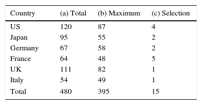
I focus on the one-year-ahead forecasts of economic growth, unemployment and inflation in the US, Japan, Germany, France, U.K. and Italy with data covering the period from January 1990 to October 2014.³ Overall, the dataset contains a large number of expert forecasters in each country (Table 1, col. a). However, we can only use a subset of these respondents. A minor problem is that some forecasters left the sample owing to closure, mergers (between banks) or other reasons, while new forecasters joined the CE survey at a later stage. A major problem is that not all economic series have received the same attention from forecasters over time, which causes some gaps in the dataset.

Table 1.

Number of forecasters in CE, January 1990–October 2014.

Country	(a) Total	(b) Maximum	(c) Selection
US	120	87	4
Japan	95	55	2
Germany	67	58	2
France	64	48	5
UK	111	82	1
Italy	54	49	1
Total	480	395	15

Notes: Total number of forecasters in CE database; and the number of forecasters that satisfy the double criterion of continuous forecasting for at least 24 months with no gaps larger than 6 months.

I therefore apply a double criterion to select the final sample. The first criterion is to eliminate those forecasters that have participated for fewer than 24 consecutive months in the CE survey. Hence, the maximum number of forecasters that produce one-year-ahead forecasts of economic growth, unemployment and inflation is smaller than the overall number of correspondents (Table 1, col. b). By the second criterion, I select from this group only those with no gaps between two consecutive forecasts that are larger than five months. Gaps of up to six months are linearly interpolated. This reduces the number of forecasters as indicated in Table 1 (col. c) to a limited set of less than 4% of the total available number. With 15 forecasters, I have 45 predictions on economic growth, unemployment and inflation over the entire time span, or a total of 13 410 observations.

2.3

Developing a new measure of global uncertainty

The measure of uncertainty is derived from these forecasts in three steps. In a first step, I compute one-year-ahead forecast errors e_t,t+1. This is the difference between the one-year-ahead forecast f_t,t+1 made in year t, and the realized data r_t+1. To that end, I collect standard measures of inflation, economic growth and unemployment for each of the six economies in the sample from the OECD Economic Outlook. I so get a complete empirical multivariate distribution of forecast errors over time.

Jurado et al. (2015) follow a distinct way to obtain the forecast error. They compute for each series the forecast error e_t,t+1 as the residual from a (time-varying stochastic volatility) FAVAR model that predicts the fit of this model as the forecast. Hence, in their case rt+1=fˆt,t+1+et,t+1. Their ex-post measure serves as a proxy for ex-ante uncertainty on the assumption that the macro-model is able to explain most of the forecastable variability in the macro-series. I adopt the same assumption. However, rather than relying on a single forecast, I assume that each forecaster has all information necessary to project the economic series, and that a forecast error is an ex-ante indication of uncertainty. This uncertainty can have its origin in multiple sources.

To examine these sources, in the second step, I summarize the information in the total number of 45 forecast error series in the dataset by extracting up to k common factors employing the method of principal factors (Stock & Watson, 2005). The forecast error e_t,t+1 on the mth observation for the nth variable can thus be written as in (1):

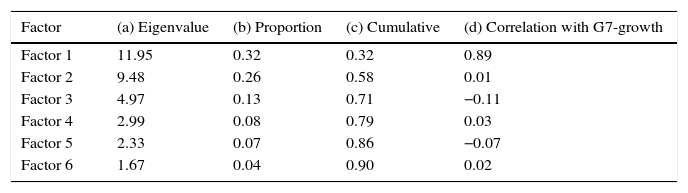
with F_m,k one of the k common factors, βk,n the corresponding factor loading and um,n the unique factor for variable n. Table 2 provides details on the factors’ unrotated loadings. According to the eigenvalues, the preferred model has six factors. The first factor explains around a third of the total variability, while the second factor accounts for about a quarter (Table 2, col. b). The remaining factors jointly explain another 30 per cent. The orthogonal or oblique rotations of the loading factors all determine that six factors are able to explain close to 90 per cent of the original series’ variability.

Table 2.

Factor model estimates on 45 series of forecast errors (see Eq. (1)).

Factor	(a) Eigenvalue	(b) Proportion	(c) Cumulative	(d) Correlation with G7-growth
Factor 1	11.95	0.32	0.32	0.89
Factor 2	9.48	0.26	0.58	0.01
Factor 3	4.97	0.13	0.71	−0.11
Factor 4	2.99	0.08	0.79	0.03
Factor 5	2.33	0.07	0.86	−0.07
Factor 6	1.67	0.04	0.90	0.02

In the final step, I characterize the possible sources of the errors forecasters make. One suggestion by the literature discussed in Section 2.1 is that cyclical fluctuations cause swings in uncertainty. Henzel and Rengel (2013) or Dovern (2015) demonstrate that the main factor driving forecast errors is correlated with business cycle conditions, and hence is actually forecastable. I find that the first factor is indeed related to the business cycle. The average growth rate across G7 economies has a close correlation of 0.89 with the first factor (see Table 2, col. d). Periods of high growth are thus associated with a rise in the first main driver in forecast errors. The second factor explains around a quarter of total variability. It is not related to cyclical developments, however, as the correlation is zero. Hence, it seems that dispersion in the opinions of forecasters has an important cyclical component.

Furthermore, I find that the factor loadings on factor 1 put the heaviest weight on the growth and unemployment forecasts, implying that most of the forecast errors are due to cyclical fluctuations. This cyclical movement in the main factor and the factor-based proxy by Jurado et al. (2015) attests to the problem detected in several empirical studies that measures of uncertainty have a clear procyclical behavior (Stock & Watson, 2012).

Other uncertainty proxies suffer from this problem too. I plot the first factor together with the similar factor-based proxy by Jurado et al. (2015) at a 12-month horizon in Fig. 1a. To make both series comparable, they are standardized. As can be seen, both measures co-move strongly. The reason is that in Jurado et al. (2015) the residual variance – or forecast error variance – is argued to reflect remaining uncertainty as all possible forecastable content is explained away by the explanatory variables in the FAVAR model that includes time lags and a number of macro-factors. Also, the time-varying stochastic volatility is responsible for any changes in residual uncertainty over time. (As a final step, aggregate uncertainty is obtained as the average of the uncertainty in each single series.) This approach does not eliminate cyclical fluctuations, however, and the FAVAR model does not incorporate all possible factors that predict business cycles. For this reason, their uncertainty measure still co-moves with the G7 business cycle.

Fig. 1.

Uncertainty measures.

Notes: Bloom measure of political uncertainty; JLN is the macro-uncertainty measure of Jurado et al. (2015) at 12 months (scaled by 100 to fit the Bloom index), and the factor-based measure based on CE forecasts.

In contrast to Jurado et al. (2015), I do not use one particular forecasting model to explain residual variance but use the entire empirical distribution of forecasts. The assumption that the ex-post realized value gives us a good indication of the forecast error is the same as in Jurado et al. (2015). There may of course be different reasons as to why forecasters are mistaken. One is cyclical fluctuations, and this demonstrates a flaw in their measure. But there can be other reasons for errors in projections by different forecasters. By filtering out the main components behind the common variance in forecast errors ex-post by applying a general factor model to the forecast errors we can examine the reasons for forecaster mistakes.

I therefore single out the second factor as reflecting the uncertainty forecasters face. A plot of this second factor in Fig. 1b shows that the factor-based measure displays somewhat more variation outside of the episodes that Jurado et al. (2015) find to be important spells of uncertainty. The reason is that by decomposing forecast errors into a notable cyclical component, I clean the dispersion of forecast errors from any strong recessionary effect. Our index argues for important spells of uncertainty in the early nineties (around the East-Asia, Russia and LTCM crisis), in late 2001, and then starting again in late 2006 (Financial Crisis), and mid-2013 (Eurozone crisis). These spikes are arguably related to important episodes of uncertainty for political reasons, as the direction of response from the policy side to big events were unknown. If we compare the factor based measure to the news index of Baker et al. (2016), our index downplays the role of uncertainty in the Financial Crisis and puts more weight on other periods. Their measure also displays substantially more variation over time than the factor-based uncertainty measure.

3

Testing the spillover effects of uncertainty

3.1

Effects of uncertainty in open economies: theory and evidence

Few structural models have been analyzed to look at the effect of uncertainty on an open economy. Fernández-Villaverde et al. (2011) set up a small open economy model and find that volatility shocks in country spreads can generate recessions. Uncertainty makes investors flee the country and hence reduce investment and growth in the short run as domestic financial markets are unable to provide smoothing.

A couple of empirical studies look into the international transmission of uncertainty. Mumtaz and Theodoridis (2012) look at how U.S. GDP growth volatility shocks spill over to the U.K. in a SVAR model with time-varying volatility, and find the effect to be sizeable. Colombo (2013) focuses on mutual spillover of U.S. and euro area policy uncertainty and the effect on economic activity. The effect of U.S. policy uncertainty shocks dominates those of euro area policy uncertainty. Klösner and Sekkel (2014) measure spillover with the Diebold-Yilmaz index and find that spillover between G7 countries explains up to one half of all movements in policy uncertainty at the height of Financial Crisis. Cesa-Bianchi et al. (2014) use a Global VAR to identify the effects of a volatility shock. Their measure covers a broad range of financial prices over 33 countries, and is driven by financial prices of over 109 assets worldwide. They assume that both volatility and real economic activity are determined by unobserved common factors, and derive then a global volatility shock. The identification assumption they maintain is that financial markets respond faster than macroeconomic developments, hence these common factors determine volatility within the period, but affect macroeconomic dynamics with a delay. They find that exogenous changes to volatility have no significant impact on economic activity, once the model is conditioned on some country-specific and global macro-financial factors.

3.2

Evidence from a panel VAR

I follow this line of literature and as Cesa-Bianchi et al. (2014), I start from a basic panel VAR model (2):

where y_i,t is a vector of endogenous variables in country i in period t, μ0i is a vector of country-specific fixed effects, A(L) is a lag polynomial with VAR coefficients and εi,t are error terms with zero mean and country-specific variances, which can be correlated with each other. The VAR contains the factor-measure of global uncertainty, private consumption and investment.

As the macroeconomic series are only available at quarterly frequency, I take the end-of-quarter value of the monthly uncertainty proxy. Domestic macroeconomic variables are from the quarterly national accounts compiled by the OECD and IMF. All series are in volumes, and deflated with a GDP deflator unless only a CPI was available. In total, I include 50 countries in the analysis,⁴ for the period of 1990Q1 to 2014Q4. This is a shorter sample period than in other studies to coincide with the factor-based measure from the CE dataset. As data are quarterly, I include four lags in the VAR.

I now write out (2) fully to get (3):

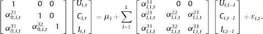
In (3), the uncertainty measure is U_i,t and I examine its effects on consumption C_i,t and investment I_i,t. Time-invariant country-specific characteristics are reflected in μi, the country-fixed effect. Identification of the model in (2) is achieved by a simple cholesky ordering. This ordering follows from the assumption that for a small open economy, global uncertainty is an external event that affects the domestic economy, but to which the country itself contributes in a negligible way (Bloom, 2009). The panel VAR can be estimated by OLS. Since the error terms are uncorrelated across equations by construction, we can estimate (1) equation by equation without loss in efficiency. I report impulse responses together with 90% bootstrapped error bands.

Estimation of the panel VAR shows that the effect of a global uncertainty shock causes a slightly negative response of investment and consumption. A rise in uncertainty produces a fall of about 2 per cent in investment, and 0.9 per cent in consumption (Fig. 2). These effects dampen out over time: we do not observe an overshooting pattern, as is typically the case for the U.S or other single-country studies. After about 5 years, the effects on consumption and investment have disappeared. These results are in line with most of the literature on the economic effects of uncertainty.

Fig. 2.

Response of consumption and investment to an orthogonalized global uncertainty shock, panel VAR, 1990Q1-2014Q3.

Notes: Unit standard deviation shock to the uncertainty index, impulse response with 90% error bands (bootstrapped).

3.3

The role of economic structure, economic policy and their interaction

The response of real activity to uncertainty shocks is not homogenous across economies. There are a few factors make that higher uncertainty in lower-income countries can in particular aggravate the consequences of uncertainty (Koren & Tenreyro, 2007). One the one hand, these are structural characteristics such as the level of financial development and the degree of diversification of an economy. On the other hand, fiscal or monetary policy choices can dampen or exacerbate the economic responses to uncertainty. These policy responses also vary with the structural characteristics. I look into four specific factors.

A first factor is that financial markets in emerging economies are not very deep. Shallow markets imply that firms and households are subject to stricter financing constraints and so exacerbate the downturn (Arellano et al., 2010). Carrière-Swallow and Céspedes (2013) estimate a VAR for a large number of countries and relate the amplitude of response with the structure of domestic financial markets. Economies with deeper markets suffer less the consequences of a shock to global uncertainty. The drop in investment is reduced by half in those emerging economies where credit flows resume quickly. This is in particular the case when firms are less dollarized. Claessens, Kose, and Terrones (2011) analyze recessionary episodes worldwide and find that they coincide more often with havoc on the financial market than happens in developed countries. Neumeyer and Perri (2005) or Uribe and Yue (2006) examine the effects of working capital constraints in a DSGE model of a small open economy, and show how these constraints deepen the impact of recessions.

A second factor that affects the spillover of uncertainty is the diversification of economies. Camanho and Romeu (2011) show that economies with more diversified sectors, and exporting a wider variety of products (albeit not necessarily to a larger number of trading partners) can significantly moderate the impact of economic crises. Emerging markets are generally less diversified than OECD countries so fluctuations in demand for a limited set of those goods can cause large swings in economic performance. Such swings can be further amplified by the composition of exports. Many emerging markets are important commodity exporters.

Uncertainty does not only keep investment or consumption decisions on hold. It also stifles the usual response of agents to policy measures. Firms and consumers are likely to respond more cautiously to interest rate cuts or fiscal stimulus when they are particularly uncertain about the future, so dampening the impact of any potential stimulus policy (Bloom, 2014). As the usual countercyclical economic policy is less effective it might actually require the stimulus to be more aggressive as it so reassures agents that the government is taking action to stabilize the economy.⁵

On the fiscal side, Ferrière and Karantounias (2016) analyze optimal fiscal policy under uncertainty and find that austerity measures that front-load fiscal consolidations are better suited as it keeps beliefs on the sustainability of public debt intact. However, hyperactive policies have often been seen as destabilizing in emerging markets, fuelling rather than calming economic uncertainty. Frankel, Vegh, and Vuletin (2013) stress the trouble of many emerging economies in pursuing countercyclical policies. Countries are often forced to adjust the budget as international credit lines are cut in a recession, and running up public debt cannot be used to smooth the impact of a shock (Mendoza & Oviedo, 2006). If the government can issue debt, then the main factor in the capacity of government to react is the fiscal space that is available. A high level of public debt might instead constrain fiscal action.

On the monetary side, activist monetary policies have been found to be reducing uncertainty, and be especially effective during financial crises if it is intervening directly on markets, as it can ease malfunctioning of financial markets for example by loosening credit constraints or restoring confidence (Bernanke & Gertler, 1995). But Bekaert et al. (2013) find that a lax monetary policy over longer times can decrease both risk aversion and uncertainty after controlling for the effect of the business cycle. But if monetary policy pushes up stock prices, continuing the loose stance may also put the seeds of a financial crisis.

For many open economies, the question of which monetary policy to pursue is closely related to the choice of the exchange rate regime (Klein & Shambaugh, 2008). A fixed exchange rate can exacerbate the financial problems of firms, in particular if companies have sought finance in the dollar. Currency mismatch and a possible depreciation expose the weak balance sheet positions of firms. Financeers prefer to wait to finance such firms. In firms facing a debt overhang, financial constraints bite deeper. If international investors flee the country in anticipation of a crisis, banks are effectively hindered from finding external finance (Calvo & Mendoza, 2000). A traditional argument in favor of flexible exchange rates is that they insulate output better from uncertainty shocks, because the exchange rate can adjust and stabilize demand for domestic goods. Moreover, if uncertainty causes investors to flee the country, a floating exchange rate may stabilize the adjustment. By contrast, with a fixed exchange rate regime, the central bank would need to intervene in support of the peg. However, a peg might import credibility from the anchor that the central bank would otherwise not possess.

The need to use policy to smooth out the effects of global uncertainty shocks depends on the financial structure of the country. With deep financial markets, it might not be necessary for fiscal policy to assume the smoothing of shocks. Credit markets are a substitute for fiscal or monetary policy. For emerging markets, fiscal policy might instead be an alternative means of stabilization if the government can borrow on behalf of households and firms. It might therefore be especially important for countries with shallow financial markets to leave sufficient fiscal space to stabilize the economy. Further, a government that has access to a well-developed domestic banking sector can easily renew public debt issues. It is harder for governments to get refinanced in an economy with a shallow financial system (Caballero & Krishnamurthy, 2004). Monetary policy might be a more efficient tool in economies with deep financial markets as the transmission mechanism is stronger. It is argued that a floating exchange rate regime would therefore be the more efficient stabilization tool in a financially developed economy (Klein & Shambaugh, 2008).

A similar argument holds for the interaction between export structure and policy. A more diversified economy is less vulnerable to uncertainty shocks. Diversified economies would give more fiscal space as tax income comes from many different sources. In the wake of heightened uncertainty, the government can still use taxes and spending to stabilize the economy. Diversification and fiscal stabilization are complements then. A diversified economic structure might require a fixed exchange rate regime to effectively stabilize trading conditions for firms.

3.4

The interacted panel VAR

Whether a similar spell of high global uncertainty is amplified or dampened by domestic policies, is therefore an empirical question to which no satisfactory answer has been given. To explore then the relevance of structural and policy characteristics – and their interaction – I introduce the Interacted Panel Vector Autoregression (IPVAR) as a framework to test the conditional response across economies to shocks in global uncertainty. This VAR model – proposed by Towbin and Weber (2013) – is similar to the panel VAR model in (3). Identification is also based on a simple cholesky ordering of the variables, and the factor-based measure of global uncertainty is considered to be predetermined with respect to variables from the domestic economy.

The interesting property of the IPVAR is that one can let the estimated coefficients vary deterministically with different characteristics of the panel units.⁶ These are either the structural economic factors X_it or the policy factors Z_it. The indicators I use to measure the structural or policy factors are the following. The aggregate index of financial development from the IMF's novel Financial Development Database (Svirydzenka, 2016) covers a wide range of countries on various aspects of the banking and credit sector. To explore the role of economic structure, I evaluate the sample for different degrees of export diversification, following the measures developed by the IMF (2014) from UN-NBER data. The measure varies between 0 and 1 with higher values indicating lesser diversification. As for fiscal policy, I measure there is sufficient space for fiscal action by taking the level of public debt as an indicator of fiscal leeway. For monetary policy, the main question for many emerging market economies has in particular been whether to pursue a fixed or a floating exchange rate. I use the (updated version of the) classification in Ilzetzki, Reinhart, and Rogoff (2010). I adapt their classification to split up the sample in countries with no exchange rate flexibility at all (dollarization, currency board, fixed peg with no band), a crawling peg (within a band), and a floating regime (managed or pure).

In order to analyze how responses vary with some characteristics of the panel units, each of the VAR coefficients (m,n) at a certain time horizon p in (3) is allowed to vary with either X_it or Z_it, and their interaction, as follows:

All terms in (4) can condition the estimated VAR coefficients. There are various ways to test the relevance of the conditioning terms for the dynamics of the transmission of uncertainty shocks.

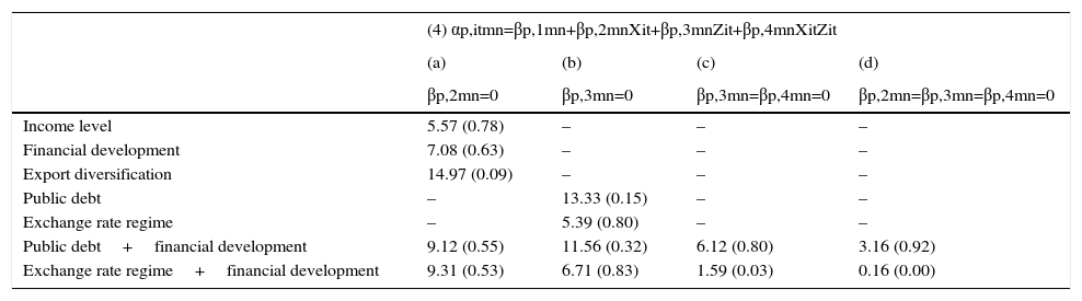
One way is to test the restrictions in (4) with a Wald-test.⁷ Four different Wald tests give an insight in the role of structural or policy factors. With a first Wald test I look only in the additional explanatory power that financial development or export diversification may give to the heterogeneity of the VAR coefficients, hence testing that βp,2mn=0 (and assuming that the other coefficients are zero). With a second test, I can similarly examine if economic policy might change the consequences of uncertainty (βp,3mn=0). The third test amounts to testing (4) and lifting the restriction on Z_it that βp,3mn=0 and βp,4mn=0. The test accounts for interaction between X_it and Z_it in (4). I.e., it is a test whether policy responses depend on structural economic characteristics. The response can go both ways. On the one hand, more activist policy can mitigate the constraints, or on the other hand, it might have exacerbated its consequences. The final Wald test has as the null that none of the terms βpmn is significant in (4). If financial development or export specialization changes the stabilization properties of policy, we should be able to reject all four null hypotheses. If structural factors have an effect on dynamics that is independent of policy, we should be able to reject the null of the first Wald test, but not of the third and fourth test.

A second way to look at the IPVAR results is to compare the impulse responses embedded in the matrix A in (2). The interaction terms make the VAR coefficients non-linear combinations. But as the error terms are not correlated across panel units, estimation can nevertheless be done by OLS. However, the impulse responses are a non-linear function of these OLS estimates, so error bounds that are bootstrapped will be more accurate than analytical ones. I report 90 per cent error bands. At what value of the conditioning characteristic X_it or Z_it to report the impulses is a matter of choice. When using continuous variables, I report impulse responses at the first (25th) percentile, the median, and a higher (75th) percentile value. The use of the first and third quartile excludes the predominant effect of outlier observations in such a heterogeneous panel of emerging and industrialized economies. For the discrete classification of exchange rates, I report the responses for the three different categories. In order to test whether the VAR model produces significant differences in the response to a specific shock at a specific time horizon, I look directly at the empirical distribution of impulse response differences and evaluate with a t-test their difference.⁸

3.5

Baseline results

Prior to checking the effect of different factors on the transmission of uncertainty, it is interesting to see how reactions differ between developed and emerging economies. Following Carrière-Swallow and Céspedes (2013), countries are classified by the World Bank classification as a high-, middle- or low-income country since 1990 (World Bank, 2015). Fig. 3 reports the impulse responses of the IPVAR for consumption and investment for these three different categories. We can infer that the response of both consumption and investment in high- and middle-income countries is rather similar, and much smoother than in low-income countries. The difference between the impulse responses of the high- and middle-income group is not statistically significant (t-test statistic, 0.53). In both groups, consumption falls by less than 1 per cent, and slowly moves back to baseline. The investment response is stronger, as it falls by around 2.5 percent at its trough after 10 quarters.

Fig. 3.

Response of consumption and investment to an orthogonalized global uncertainty shock, panel VAR, 1990Q1-2014Q3, by different levels of income (World Bank, 2015).

Notes: Unit standard deviation shock to the uncertainty index, impulse response with 90% error bands (bootstrapped).

By contrast, in low-income countries, the drop in consumption is about 3 per cent, and in investment close to 6 per cent. A t-test on the difference between the impulse response functions with the middle-income group shows a significant difference in consumption over the 20 quarters at the 5 per cent significance level (t-test statistic: 2.28). As the error bands are wider for investment, the response is found to be significantly different at the 10 per cent level only (t-test statistic: 1.69). A Wald-test shows that we can clearly reject the null that income levels do not explain differences in responses (Table 3, col. a).

Table 3.

Wald-tests on interaction terms: test-statistic and p-value (in brackets).

	(4) αp,itmn=βp,1mn+βp,2mnXit+βp,3mnZit+βp,4mnXitZit
	(a)	(b)	(c)	(d)
	βp,2mn=0	βp,3mn=0	βp,3mn=βp,4mn=0	βp,2mn=βp,3mn=βp,4mn=0
Income level	5.57 (0.78)	–	–	–
Financial development	7.08 (0.63)	–	–	–
Export diversification	14.97 (0.09)	–	–	–
Public debt	–	13.33 (0.15)	–	–
Exchange rate regime	–	5.39 (0.80)	–	–
Public debt + financial development	9.12 (0.55)	11.56 (0.32)	6.12 (0.80)	3.16 (0.92)
Exchange rate regime + financial development	9.31 (0.53)	6.71 (0.83)	1.59 (0.03)	0.16 (0.00)

To explore then the relevance of financial development, I evaluate the sample at the 25th, median and 75th percentile level of financial development. Plots of the impulse response functions in Fig. 4 show that in countries with more developed financial systems, the effects of uncertainty shocks are hardly significant. By contrast, we observe pronounced falls in consumption and investment in countries with a median level of financial development of about 1 and 3 per cent, respectively. An even stronger drop happens in countries at very low levels of development, as they experience a fall in consumption of about 2 per cent, and in investment of about 6 per cent. A t-test shows the response to be significantly different at 5 per cent between all groups. A Wald-test also rejects the null that financial development is not relevant in explaining cross-country differences (Table 3, col. a). The importance of the depth of financial markets is a result that is in line with other studies (Carrière-Swallow & Céspedes, 2013).

Fig. 4.

Response of consumption and investment to an orthogonalized global uncertainty shock, panel VAR, 1990Q1-2014Q3, by level of financial development (Svirydzenka, 2016).

Notes: Unit standard deviation shock to the uncertainty index, impulse response with 90% error bands (bootstrapped).

To further explore the role of economic structure, I then evaluate the sample for different degrees of export diversification. Fig. 5 shows few differences between the impulse responses at different levels of diversification. Economies that are at the lowest quartile of diversification suffer a fall that is somewhat stronger as for economies on the third quartile of the distribution. A Wald-test rejects the null that the response is not dependent on this conditioning factor, albeit at the 10 per cent level only (Table 3, col. a).

Fig. 5.

Response of consumption and investment to an orthogonalized global uncertainty shock, panel VAR, 1990Q1-2014Q3, by export diversification (IMF, 2014).

Notes: Unit standard deviation shock to the uncertainty index, impulse response with 90% error bands (bootstrapped).

I can then test whether policy reactions in different groups of countries dampen or exacerbate the role of other conditioning factors. I first do so by only examining the policy factor Z_it to condition the responses of the VAR model. In the case of fiscal policy, the level of public debt conditions the response across countries strongly. Perhaps surprisingly, at low levels of public debt, the response to an uncertainty shock is seen to be substantially stronger (Fig. 6). The fall in consumption is 2 per cent, and in investment about 6 per cent. By contrast, in a high debt country, the response is hardly significant on both consumption and investment. These differences are statistically also very significant. A Wald test confirms that we cannot reject that public debt has an impact on the transmission of uncertainty shocks.

Fig. 6.

Response of consumption and investment to an orthogonalized global uncertainty shock, panel VAR, 1990Q1-2014Q3, by level of the public debt ratio.

Notes: Unit standard deviation shock to the uncertainty index, impulse response with 90% error bands (bootstrapped).

For different exchange regimes, I use the measure developed in Ilzetzki et al. (2010). Fig. 7 shows the impulse responses for the three categories. The fall in consumption and investment is much stronger in the countries with a floating regime. Even if the differences in the responses are tiny, the t-tests show a significant difference at 1 per cent.⁹ In the floating regime, investment falls by up to 4 per cent, whereas it is more limited in the more fixed regimes. This is further confirmed by a Wald-test.

Fig. 7.

Response of consumption and investment to an orthogonalized global uncertainty shock, panel VAR, 1990Q1-2014Q3, by type of exchange rate regime (Ilzetzki et al., 2010).

Notes: Unit standard deviation shock to the uncertainty index, impulse response with 90% error bands (bootstrapped).

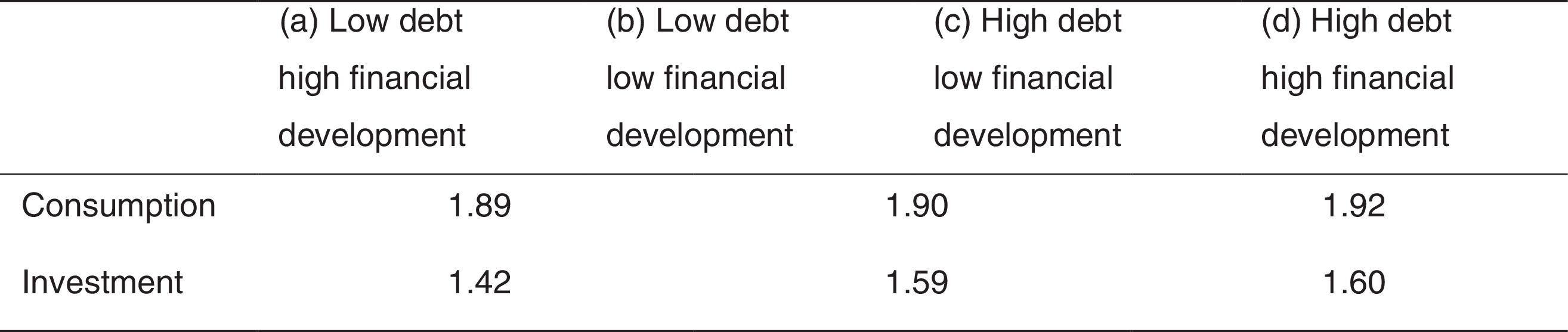
What lies behind these differences? Policy reactions might be conditioned by the economic structure of the economy. I thus look into the effects of an uncertainty shock for different levels of debt and different degrees of financial development. The four possible combinations shown in columns (a)–(d) of Fig. 8 are: ‘low debt/highly developed’, ‘low debt/lowly developed’, ‘high debt/lowly developed’, and ‘high debt/highly developed’ at the relevant quartiles of their distributions.

Fig. 8.

Response of consumption and investment to an orthogonalized global uncertainty shock, panel VAR, 1990Q1-2014Q3, by level of public debt ratio and financial development.

Notes: Unit standard deviation shock to the uncertainty index, impulse response with 90% error bands (bootstrapped).

Let us look at the first two columns for countries with low debt. Financial development matters in the transmission of the shock, as a developed financial system copes well to mitigate the effects of uncertainty. At low levels of public debt, the effect is actually nil. The responses to an uncertainty shock are still muted when financial development is not as high but debt is low.

The role of financial development is much stronger at high debt levels, however. In that case, the consequences of an uncertainty shock are much stronger in a less developed financial system than in a well developed one. Investment falls by about 18 per cent, and consumption by about 8 per cent (albeit the responses are not very significant as the error bands are very large). Even for an economy at high levels of financial development, a high public debt causes a significantly stronger contractionary response in consumption and investment to an uncertainty shock. As shown in Table 3 (cols. c and d), all interaction terms are jointly significant according to a Wald test. Table 4 reports the t-tests on the differences in the impulse responses between the different groups. These are not always significant, not even at 10 per cent, but this is a result of the wide error bands in column (c) of Fig. 8. These tests imply that the interaction between fiscal policy and financial development is relevant in explaining cross-country differences in the response to uncertainty shocks.

Table 4.

T-test on difference in impulse response functions: test-statistic.

Notes: t-test on difference between combinations of financial development and public debt: between (a)–(b), (b)–(c) and (c)–(d).

It points at an important role for fiscal policy in economic stabilization that we could not infer from Fig. 6 as such. There, we found that high debt is associated with a muted response to uncertainty. Fig. 8 tells us that this response is only possible if an economy's financial system is developed enough to allow for the smoothing of shocks. A country with a not very developed financial system would need much more fiscal space to tackle the consequences of uncertainty shocks. This result points to a trade-off: one the one hand, using fiscal policy would be useful to dampen the effects of uncertainty, but if financial markets are not ready to take up the issuance of bonds, then this is hard to realize. This evidence endorses the view that fiscal policy might be useful to smooth out shocks if financial markets are unable to take on its effects.

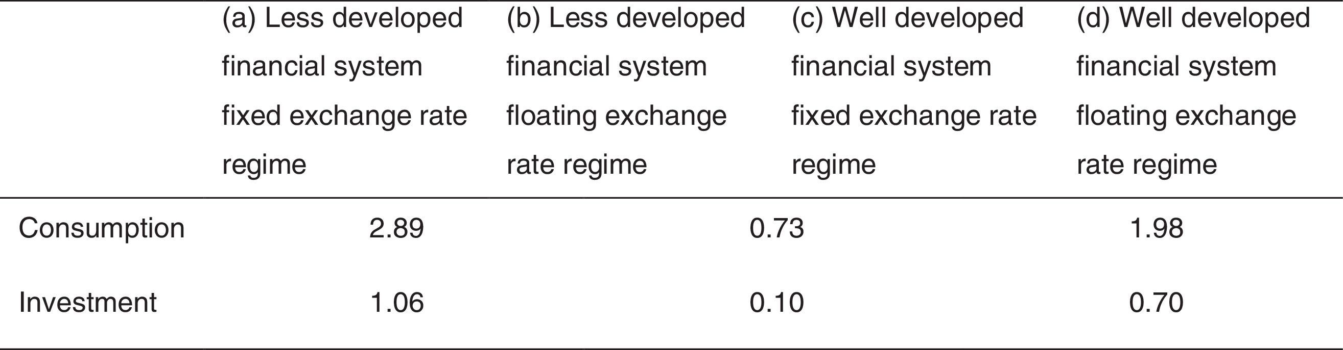
The same exercise for different combinations of the exchange rate regime and the level of financial development shows in Fig. 9 in the first two columns the reactions to an uncertainty shock for low financial development, and in the last two columns for high financial development. I just plot the extreme two cases of a fixed peg or a floating regime. Remember that in Fig. 7, the reaction of consumption and investment was stronger under the floating regime.

Fig. 9.

Response of consumption and investment to an orthogonalized global uncertainty shock, panel VAR, 1990Q1-2014Q3, by type of exchange rate regime and financial development.

Notes: Unit shock to the uncertainty index, impulse response with 90% error bands (bootstrapped).

For countries with less developed financial system, the responses to uncertainty are much faster and deeper in a floating exchange rate regime. Instead, under a fixed peg, the response is dampened. It does not matter a lot whether the financial system is well developed or not, as the last two columns of Fig. 9 show. The responses to an uncertainty shock are as strong – but less significant – at high levels of financial development. This result seems to suggest that the monetary policy response is not so much connected to the level of financial development. In fact, a Wald test does reject the null that the interaction term between both characteristics is relevant for the transmission of uncertainty shocks (Table 3, cols. c and d). Table 5 further shows that cross-country differences in the response to uncertainty shocks do not depend on the choice of the exchange rate regime. The t-test on the difference between the impulse response functions from the fixed to the floating group is just marginally significant, except for consumption.

Table 5.

T-test on difference in impulse response functions: test-statistic.

Notes: t-test on difference between combinations of financial development and public debt: between (a)–(b), (b)–(c) and (c)–(d).

The results show that in the wake of uncertainty, a fixed peg may actually result in an easier adjustment of the economy. The result is quite different in a floating regime: a more flexible policy stance is not recommendable to stabilize the economy. The choice seems to depend on how countries can cope with uncertainty: a fixed peg may be seen as a more credible commitment to a stability-oriented policy. It seems that with uncertainty, a less flexible exchange rate regime puts monetary policy in the position to stabilize the economy.

3.6

Robustness checks

There is a possibility that the results on policy intervention in the panel VAR model are driven by crisis episodes, thus exaggerating the difference for high debt countries or those with floating exchange rate regimes. A common global uncertainty measure might not fit well with emerging markets, as idiosyncratic events may be responsible for major deviations. Domestic uncertainty that results from economic or policy events may be the main driver of the responses.

Few measures of uncertainty have been developed for emerging markets (Cerda et al., 2016). Hence, I include as an alternative different financial crisis episodes as exogenous variables to the VAR. I take the financial crisis classification from Laeven and Valencia (2013), who use a narrative approach for identification of the episodes, and add each episode as a dummy to the VAR. The differences are not influenced by the crisis episodes, as the impulse responses are very similar to those in Figs. 6–9.¹⁰

4

Conclusion

Spells of uncertainty are argued to cause rapid drops in economic activity. Wait and see behavior and risk aversion in combination with other frictions can make these periods of increased uncertainty an important driver of the business cycle. Emerging economies may endure stronger and prolonged recessions following a global uncertainty shock. Credit constraints in shallow financial markets in small open economies trigger deeper recessions. Policy reactions might exacerbate those episodes.

This paper develops a novel proxy of uncertainty – a common factor from a large database of forecaster projections in G7 countries – that is less subject to business cycle endogeneity than other proxies for uncertainty. I then estimate an interacted panel VAR on a large set of developed and emerging economies over the period 1990Q1-2014Q3 to test the economic responses to shocks to uncertainty conditional on structural and policy conditions.

Emerging markets do suffer larger and more prolonged falls in consumption and investment as uncertainty spreads globally, as also Carrière-Swallow and Céspedes (2013) detected. This seems closely linked to the development of financial markets: the transmission of uncertainty is significantly dampened if financial markets are deep enough so households and firms can smooth the effect of the uncertainty shock. If fiscal policy has a capacity to act and keeps debt under control, the negative effect is further dampened. There is no evidence of a strong interaction between the choice of the exchange rate regime and financial development. A floating exchange rate accelerates the response to a crisis whereas a fixed peg shields economies from the spillover of uncertainty shocks.

The empirical findings imply that financial development is the key element for the transmission of global uncertainty shocks. Policies to broaden and deepen the domestic financial sector would make emerging countries much more resilient to global uncertainty, and likely other shocks as well. Fiscal policy would not face such a difficult trade-off between “policy correctness and decisiveness” (Bloom, 2009). More financial development would enable emerging economies to run more countercyclical policies without endangering sustainability in the longer term, so that at times of heightened uncertainty, more policy activism could be used diligently. Rules that constrain debt-buildup or let monetary policy follow a clear strategy, would allow firms and households to continue implement their plans without additional uncertainty.

Conflict of interests

The author declares that they have no conflict of interest.